Three-point functions and su(1 vertical bar 1) spin chains

JHEP09(2014)173

Received_: July 30, 2014

Accepted_: September 3, 2014

Published_: September 29, 2014

Three-point functions and

su

(1

|

1)

spin chains

Jo˜ao Caetanoa,b,c and Thiago Fleuryd a

Perimeter Institute for Theoretical Physics, Waterloo, Ontario N2L 2Y5, Canada b

Department of Physics and Astronomy & Guelph-Waterloo Physics Institute, University of Waterloo,

Waterloo, Ontario N2L 3G1, Canada c

Centro de F´ısica do Porto e Departamento de F´ısica e Astronomia, Faculdade de Ciˆencias da Universidade do Porto,

Rua do Campo Alegre, 687, 4169-007 Porto, Portugal d

Instituto de F´ısica Te´orica, UNESP — Univ. Estadual Paulista, ICTP South American Institute for Fundamental Research,

Rua Dr. Bento Teobaldo Ferraz 271, 01140-070, S˜ao Paulo, SP, Brasil

E-mail: jd.caetano.s@gmail.com,tfleury@ift.unesp.br

Abstract: _{We compute three-point functions of general operators in the su(1|1) sector} of planar _N = 4 SYM in the weak coupling regime, both at tree-level and one-loop. Each operator is represented by a closed spin chain Bethe state characterized by a set of momenta parameterizing the fermionic excitations. At one-loop, we calculate both the two-loop Bethe eigenstates and the relevant Feynman diagrams for the three-point functions within our setup. The final expression for the structure constants is surprisingly simple and hints at a possible form factor based approach yet to be unveiled.

Keywords: _{Supersymmetric gauge theory, 1/N Expansion, Bethe Ansatz, Integrable}

Field Theories

JHEP09(2014)173

Contents

1 Introduction 1

2 Three-point functions at leading order 3

2.1 The one-loop Bethe eigenstates and structure constants 6

3 One-loop three-point functions 9

3.1 Two-loop coordinate Bethe eigenstates and norms 9

3.2 One-loop perturbative calculation 11

3.3 Final result 14

4 Discussion and open problems 15

A Notation and conventions 17

B One-loop perturbative computation details 18

C Some examples of three-point functions 24

C.1 Three half-BPS operators 24

C.2 Two non-BPS and one half-BPS operators 26

D Wilson line contribution 29

D.1 Wilson line connecting two scalars 30

D.2 Wilson line connecting either a scalar and a fermion or two fermions 30

E A note on the su(1|1) invariance of the final result 30

1 Introduction

Integrability has proven to be a powerful tool for studying the planarN = 4 SYM theory. In particular, it was successfully used to compute all the two-point functions of the gauge-invariant single-trace operators for any value of the ’t Hooft parameterλ, see for instance [1– 3]. The predictions from integrability have been extensively tested and they correctly reproduce the known results obtained in perturbation theory at weak coupling and the ones obtained by the AdS/CFT conjecture in the strong coupling limit.

JHEP09(2014)173

Sector Tree-level and

Integrability

One-loop

prescription

One-loop and

Integrability

Higher

loops

su(2) [4,5] [6,7] [8,9] unknown

sl(2) [10,11] [7] (some cases) [10] (some cases) [12,13]

su(1_|1) here here here unknown

so(6) [14] (some cases) [6,7] unknown unknown

psu(2,2_|4) unknown unknown unknown unknown

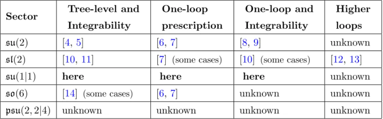
Table 1. The current status of the computation of three-point functions.

A single-trace operator of _N = 4 SYM is thought of as a closed spin chain state. To leading order in the ’t Hooft coupling these spin chain states are very well understood and given by the so-called Bethe ansatz. The problem at tree-level is purely combinatorial and amounts to cutting and sewing such spin chains. At the end of the day, this boils down to a computation of some scalar products of Bethe states. Nevertheless, this is a very rich and non-trivial problem. For instance, scalar products between Bethe states in higher rank algebras are not known. It is therefore so far unclear how to perform the computation of the most general psu(2,2|4) correlators as indicated by the last row of table1.

This motivates one to start studying the rank one sectors in a systematic way. They consist of thesu(2),su(1_|1) and sl(2) sectors and they played a very important role in the spectrum problem, see for instance [15]. The first three rows of the table 1 summarize the current knowledge on these sectors. In the su(2) case, the final result for the structure constants turns out to be given in terms of determinants depending on three sets of numbers called Bethe rapidities while in thesl(2) sector, it was found a formula given in terms of a sum over partitions of these Bethe rapidities. In this paper, we will study the remaining rank one sector.

Whichever sector we consider, there are, at one-loop, two effects that need to be taken into account.

• Firstly, there is the two-loop correction to the Bethe state, which is of order λ and thus contributes to the one-loop structure constant. This amounts to correct not only theS-matrix but also modifying the Bethe ansatz itself by introducing the so-called contact terms. These are required due to the long-range nature of the dilatation operator which couples non-trivially neighboring magnons on the spin chain. In this regard, some surprises were found recently. The contact terms were found to be ultra-local in sl(2) and much simpler than in thesu(2) case. In this paper we find a remarkably simple form for the contact terms insu(1_|1) allowing us to fully construct the two-loop Bethe state for an arbitrary number of magnons.

JHEP09(2014)173

partial results were obtained in [7] but the complete computation remains to be done. In this paper, we provide the complete one-loop prescription for the su(1_|1) sector.

In the end, combining both loop contributions for su(1_|1), we found a strikingly sim-ple formula for the one-loop structure constant C123. Given three operators Oi with Ni

excitations with momenta {p(_ji)_}Ni

j=1, and length Li (the details of the exact setup will be

given below), we have

C123=C 3 Q

i=1

Ni

Q

j<k

f(y(_ji), y(_ki))

N1

Q

i=1

N2

Q

j=1

f(y_i(1), y_j(2))

N1

Y

k=1

"

1₋(y(1)_k )L2

N2

Y

i=1

−S(y_i(2), y_k(1)) #

, (1.1)

where y_j(i) _≡ eip(i)j _{, C is a simple normalization factor given in (3.14), S is the su(1|1)S} -matrix. The most essential ingredient and main result of this work is the functionf which is simply given by

f(s, t) = (s₋t)

1₋ g 2

2

s t +

t s−

1 s−s−

1

t −t+ 2

+_O(g4)

, (1.2)

withg2= λ

16π2.

The paper is organized as follows. In section 2, we explain the three-point function setup that will be used in the remaining of the paper and compute the leading contribution to the structure constants in terms of a simple expression which is function of the momenta of the excitations. Section 3 is devoted to the calculation of the one-loop corrected struc-ture constants. The section begins with the construction of the two-loop eigenstates by computing the contact terms, then we evaluate the relevant Feynman diagrams needed for determining the prescription for computing the one-loop corrections. In the end, we put the different contributions together and we arrive at the formula (1.1). Finally, the section 4 contains our conclusions and perspectives. Several appendices have additional details omitted during the presentation.

2 Three-point functions at leading order

In this section, we perform the computation of the structure constants at leading order. The setup that will be used for the calculation involves composite operators made out of both fermionic and scalar fields. Each of these operators is thought of as a state of a closed spin chain with the fermionic fields being excitations over a ferromagnetic vacuum. The ad-vantage of this approach is that the connection with the integrability tools of quantum spin chains becomes manifest (see for instance [2]) and facilitates the combinatorial problem.

JHEP09(2014)173

{ , {

{ , {

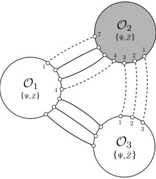
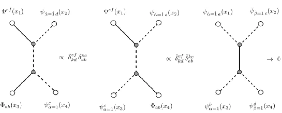
Figure 1. The leading order contribution to the three-point functions. The solid lines represent bosonic propagators and the dashed lines represent fermionic propagators. We also indicate our conventions for labeling the positions of the excitations. Notice that in our setup the first N3

excitations of the operator_O2 have always their position fixed.

functions that we will be considering involves an operator_O1 given by a linear combination of single traces made out of products of these fields. More precisely,

O1 =

X

1≤n1<n2<...<nN₁≤L1

ψ(1)(n1, n2, . . . , nN1) Tr

Z . . . Ψ

n1

. . . Ψ

n2

. . . Z

, (2.1)

whereL1 is the length of the operator, N1 is the number of its fermionic fields and n’s are the positions of the excitations along the chain of Z’s. We designate the coefficients ψ(1) in this linear combination by wave-function. It is natural to consider the second operator O2 made out of the complex conjugate fields, namely

O2 =

X

1≤n1<n2<...<nN₂≤L2

ψ(2)(n1, n2, . . . , nN2) Tr

¯ Z . . .Ψ¯

n1

. . .Ψ¯

n2

. . .Z¯

. (2.2)

In our conventions, the complex conjugate fields are given by

¯

Z = (Z)∗ =Φ34=Φ12, (2.3)

¯

Ψ = (Ψ)†= ¯ψ_{4,α˙= ˙1}.

From now on, we will omit the Lorentz spinorial indices at several places keeping in mind that they are always kept fixed.

As a consequence of theR-charge conservation, it is clear that we cannot take the third operator to be also in the same su(1_|1) sector to which _O1 and O2 belong, if we want to have a non-vanishing result and avoid extremal correlation functions.1 Instead, we consider

JHEP09(2014)173

operator of the typeO1. The idea is to get a composite operator having a term with onlyΨ and ¯Zfields in order to allow non-vanishing Wick contractions between all pairs of operators (see figure1 for an example of a non-extremal three-point function). More precisely, let us suppose that we start with a state made out ofΨ andZ fields. In order to convert a single Z into a ¯Z we must apply a pair of su(4) generators that rotate its twoR-charge indices. In sum, we can generate a term withΨ’s and ¯Z’s by considering the following operation

O3 =

1 (L3−N3)!2

(R2₄R1₃)L3−N3 X

1≤n1<...<nN₃≤L3

ψ(3)(n1, . . . , nN3) Tr (Z . . . Ψ . . . Ψ . . . Z) , (2.4) whereRa

b aresu(4) generators and they act on the fields inside the trace. Now, thesu(4)

generators may also act on the field Ψ which carries oneR-charge index. Therefore, this operation will generate several terms coming from the different ways of acting with the generators,

O3 =

X

1≤n1<...<nN₃≤L3

ψ(3)(n1, . . . , nN3) h

Tr ¯Z . . . Ψ . . . Ψ . . .Z¯+

+ Tr ¯Z . . . ψ2. . . Ψ . . . Φ14+. . .i, (2.5)

where in the first line we have the term where all the su(4) generators act on the scalar fieldsZ. In the second line, we represent the terms where some of the generators also act on the fermionic fieldsΨ. As an example of how the formula given above is evaluated consider,

(R2₄R1₃)_·Tr (Ψ Z) = (R2₄R1₃)_·Tr (ψ4Φ34) = Tr (ψ2Φ14) + Tr (ψ4Φ12).

At tree-level, the terms in the second line of (2.5) do not give any contribution due to the R-charge conservation. In other words, one always has a zero Wick-contraction. Therefore, at leading order, only the first line contributes and we get a tree-level diagram of the type represented in figure1. At one-loop, the terms in the second line will also need to be taken into account. We emphasize that the operators O1 in (2.1) and O3 in (2.4) are spinorial operators with N₁ and N₃ indices α = 1 respectively. This follows from the definition of the field Ψ given previously. The operator_O2 in (2.2) hasN2 Lorentz indices

˙

α= ˙1 associated to each of the fermions ¯Ψ.

In a conformal field theory, the two-point functions are completely fixed by the symme-tries up to a normalization constant. For two operators having spinorial indices as shown below, we have

hOi; 11...1Ni(x1) ¯Oi; ˙11...˙1_Ni(x2)i=Ni

(J_{12,1 ˙1})Ni |x12|2∆i

, (2.6)

where_Ni is a constant associated to the normalization of the operator, ∆i is its conformal

dimension and the tensorial structure is2

J_{ij,1 ˙1}= x

µ

ij σEµ

1 ˙1 (2π)2|xij|

JHEP09(2014)173

has many inequivalent tensor structures consistent with the conformal symmetry, and the result of the correlation function is a linear combination of these structures. The constraints following from conformal symmetry on the higher point functions were studied for instance in [16–18]. However, for the setup considered in this work there is only one possible tensor and the three-point functions are of the form

hO1;11...1N₁(x1)O2; ˙11...˙1N₂(x2)O3;11...1N3(x3)i= (2.8) = (J12,1 ˙1)

N1_(J

23,1 ˙1)N3 √

N1N2N3C123(g2) |x12|∆1+∆2−∆3|x13|∆1+∆3−∆2|x23|∆2+∆3−∆1

,

where we are consideringN2 =N1+N3 and g2= ₁₆λ_π2 withλthe ’t Hooft parameter. The structure constant C123(g2) has a perturbative expansion when g2 is small, and its leading order will be designated byC₁₂₃(0). Using the figure1, we observe that the only non-trivial Wick contractions occur between operators_O1 andO2. The structure constant C₁₂₃(0) is then given by the product of the three wave-functions with a sum over the positions of the excitations between these two operators,

C

(0) 123 =α

ψ₁(3)_,...,N

3

X

N3<n1<...<nN₁≤L2

ψ_L(1)

2+1−nN₁,...,L2+1−n1ψ

(2)

1,...,N3,n1,...,nN₁

. (2.9)

αis a normalization factor that comes from the fact that we are normalizing the operators such that their two-point functions have the canonical form (2.6) with_Ni = 1. It is given by

α= r

L1L2L3

N(1)_N(2)_N(3), with N

(j)₌ X

1≤n1<...<n_Nj≤Lj

(ψ(_nj₁)_,...,n

Nj) ∗_(ψ(j)

n1,...,n_Nj). (2.10)

The main goal of this section is to find a closed formula forC₁₂₃(0).

2.1 The one-loop Bethe eigenstates and structure constants

To computeC₁₂₃(0) we must consider states with definite one-loop anomalous dimension [4]. The one-loop su(1_|1) integrable Hamiltonian and S-matrix can be found in [15,19]. The Hamiltonian is simply the fermionic version of the Heisenberg Hamiltonian and it is written in terms of the Pauli matrices as

H1= 2g2

L

X

n=1

(1₋σ3_n)₋1 2(σ

1

nσ1n+1+σ2nσ2n+1)

, (2.11)

where L is the length of the spin chain. At leading order the two-excitation S-matrix is independent of their momenta and simply given by

S(p1, p2) =−1. (2.12)

In order to find the eigenstates of the Hamiltonian given above, we use the usual coordinate Bethe ansatz. A N-magnon state of a spin-chain of lengthLis of the form

|ψNi=

X

1≤n1<n2<...<nN≤L

JHEP09(2014)173

chain (for details about the coordinate Bethe ansatz see [2, 4]). Notice that the ket |n1, . . . nNi represents the trace in (2.1). The wave-function ψN(n1, . . . , nN) is a

com-bination of plane waves with as many terms as the number of possible permutations of the momenta with the relative coefficients being theS-matrices. Since the leading ordersu(1|1) S-matrix is just ₋1, the several terms in the wave-function will appear with alternating signs which we write as

ψN(n1, n2, . . . , nN) =

X

P

signP exp(ipσP(1)n1+ipσP(2)n2+. . .+ipσP(N)nN) (2.14) where P indicates sum over all possible permutations σP of the elements{1, . . . , N}, and

signP is the sign of the permutation. Moreover, we should impose the periodicity condition by requiring the momenta pi to satisfy the Bethe equations

eipiL_{= 1. (2.15)}

The cyclic property of the trace is implemented by imposing the zero momentum condition of the state,

N

X

i=1

pi = 2π×integer. (2.16)

Having determined the eigenstates of the one-loopsu(1_|1) Hamiltonian, we can proceed to compute the leading order structure constantC₁₂₃(0) given in (2.9) by following some simple steps. Firstly, we notice that since the positions of the excitations of the third operator are fixed, we can use (2.14) to write ψ(3) explicitly. It is simple to see that we obtain a Vandermonde determinant which can be also presented as a simple product,

C

(0) 123 =α

N3

Y

j<k

eip(3)j −_eip (3) k

X

N3<n1<...<nN₁≤L2

(ψ_n(1)_1,...,n

N₁) ∗_ψ(2)

1,...,N3,n1,...,nN₁

. (2.17)

Moreover we have replaced ψ_L(1)

2+1−nN₁,...,L2+1−n1 by (ψ

(1)

n1,...,nN₁)∗ since they differ by at

most a sign.

Notice that the first N3 excitations of the wave-functionψ(2) have their positions fixed orfrozen. In order to make the computation of this sum simpler, we consider an auxiliary problem where we addN₃ extra excitations to the wave-functionψ(1)and liberate the fixed N3 excitations ofψ(2) with their positions being summed over too,

Saux ≡

X

1≤n1<...<nN₃₊N₁≤L2

(ψ_n(1)_1,...,nN

3+N₁) ∗_ψ(2)

n1,...,nN₃₊N₁. (2.18)

The advantage of considering this auxiliary problem is that the sum (2.18) can be easily computed due to the form of the wave-functions. Moreover, we can relate it with the original sum appearing in (2.17) as we now explain. Indeed, let us consider thatN3 momenta, say {p(1)₁ , . . . , p(1)_N

JHEP09(2014)173

More precisely, we send {e−ip(1)_{1 , . . . , e}−ip(1)N_{3} to zero in such a way that}

e−ip(1)1 ≪ · · · ≪_e−ip (1)

N_{3 . (2.19)}

Thus, given the explicit form of the wave-function (2.14), we observe that in this limit the sum over the positions of the extra roots in (2.18) is dominated by the term for which n1 = 1, . . . , nN3 = N3. This procedure of sending roots to a particular limit in order to freeze their positions is the coordinate Bethe ansatz counterpart of thefreezing trick used in [5] at the level of the six-vertex model. Neglecting all the subleading terms, we get that in this limit, (2.18) is reduced to

Saux→

N3

Y

k=1

e−ip(1)k k !

X

N3<n1<...<nN₁≤L2

(ψ(1)_n1,...,nN

1) ∗_ψ(2)

1,...,N3,n1,...,nN₁, (2.20)

where we recognize precisely the original sum of (2.17).

Returning to our auxiliary problem, we use again that the wave-function is completely antisymmetric in its arguments to extend the limits of the sum (2.18). In compensation, we merely have to introduce a trivial overall combinatorial factor. Using the explicit form of the wave-function we write the sum (2.18) as

Saux = 1 N2!

X

{ni} X

P,Q

signPsignQ

N1+N3

Y

a=1

e

ip(2)_P(a)−ip(1)_Q(a)na

. (2.21)

We emphasize again that we now sum without restrictions, 1 _≤ ni ≤ L2, for all ni.

These sums over ni can be explicitly computed as they are geometric series. Using the

Bethe equations and the total momentum condition for the operator O2, we can then simplify (2.21) to

Saux =

"_N1+N3 Y

a=1

1₋e−ip(1)a L2 #

1 N2!

X

P,Q

signPsignQ

N1+N3

Y

a=1

1

eip

(1) Q(a)_−eip

(2) P(a)

. (2.22)

The remaining sum in the previous expression is manifestly the definition of a Cauchy determinant and, therefore, it can be written explicitly as a simple product as follows

Saux =

"_N1+N3 Y

a=1

1−e−ip(1)a L2 # Q

j<k

(eip(1)j −_eip (1) k )(eip

(2) k −eip

(2) j )

Q

j,k

(eip(1)j −_eip(2)k )

. (2.23)

Notice that this expression contains as a limit the norm of an operator.3 It is given by

N(j) =LNj

j . (2.24)

3_{If we considerp}(1) j →p

(2)

j we get the expression forN

JHEP09(2014)173

Plug-ging the resulting limit and taking into account the overall product multiplying the sum in (2.20), we obtain our final result

C (0) 123 = " ₃ Y i=1 L

1−Ni

2 i #   N1 Y j=1

1−eip(1)j L2   3 Q a=1 Na Q j<k

(eip(a)j −_eip (a) k )

N1

Q

j=1

N_Q2

k=1

(eip(1)j −_eip (2) k ) . (2.25)

It is now straightforward to confirm that our formula (1.1) given in the introduction, reduces to this one when g is set to zero.

This result fills the first column for the su(1_|1) row of the table1 in the introduction. Let us remark that this expression is considerably simpler than the ones found for thesu(2) andsl(2) sectors. This is perhaps not surprising given that at leading order we are dealing with a theory of free fermions so that the form of thesu(1_|1) wave-function becomes quite simple. However, we will see that the one-loop result persists to be simpler than in the other sectors.

3 One-loop three-point functions

In this section, we compute the structure constants at first order in the ’t Hooft coupling λ for our setup. There are two main ingredients in this computation. Firstly, one has to consider Bethe eigenstates that diagonalize the two-loop dilatation operator as these states are of orderλ. Secondly, one has to compute the relevant Feynman diagrams at this order in perturbation theory. This second contribution can be compactly taken into account through the insertion of an operator at specific points of the spin chains as will be reviewed.

3.1 Two-loop coordinate Bethe eigenstates and norms

The two-loop Bethe eigenstates are determined by diagonalizing the long-range Hamilto-nianH [15]

H=H₁+H₂, (3.1)

whereH1 is given in (2.11) and

H2 = 4g2

L

X

n=1

2(σ_n3₋1)₋1 4(σ

3

nσn3+1−1) + (σn1σn1+1+σn2σ2n+1) 9 8 − 1 16σ 3 n+2 (3.2) −1 16σ 3

n(σn1+1σn1+2+σn2+1σn2+2)−

1 8σ

1

n(1 +σ3n+1)σn1+2−

1 8σ

2

n(1 +σn3+1)σ2n+2

!

,

where σi are the Pauli matrices. In order to diagonalize it, we start with the usual coor-dinate Bethe ansatz which works when the excitations are at a distance bigger than the range of the interaction, i.e. when |ni−nj|>2. In this region all we need is the two-loop

S-matrix which reads

S(p1, p2) =−1−8ig2sin _p1

2

sin

p1−p2 2

sinp2 2

JHEP09(2014)173

wave-function to be modified with respect to the usual Bethe ansatz (2.14). In fact, when magnons are placed at neighboring positions on the spin chain they interact in a non-trivial way. Therefore, the wave-function must be refined by the inclusion of the so-called contact terms. For instance, in the case of three magnons we write it as

ψ(n1, n2, n3) =φ123+φ213S21+φ132S32+φ312S31S32+φ231S31S21+φ321S32S31S21,

where we have used the notationSab =S(pa, pb) and

φabc = eipan1+ipbn2+ipcn3

1 +g2C₍pa, pb)δn2,n1+1δn3>n2+1+g

2_C(p

b, pc)δn2>n1+1δn3,n2+1

+g2C_{(pa, pb, pc)δn}

2,n1+1δn3,n2+1

. (3.4)

The functions C _{are the contact terms which are fixed by solving the energy eigenvalue} problem. In the case of N-magnons, the wave-function has a similar structure. It consists of N! terms coming from the permutations of {p₁, . . . , pN} and N −1 types of contact

terms namelyC_{(pi, pj), . . . ,}C_{(p1, . . . , pN).}

Unexpectedly, we have found that up to seven magnons the contact terms are simply given by4

C_{(p1, . . . , pn) =} n−1

2 . (3.5)

Even though we have not proved the validity of this formula for an arbitrarily high number of magnons, the pattern emerging up to seven magnons is quite suggestive. Given the form of the contact terms in thesu(2) andsl(2) sectors, the simplicity of thesu(1|1) result is quite surprising. In particular, notice that they are independent of the momenta of the colliding magnons. This might be pointing towards the existence of a new algebraic description of these states yet to be unveiled.

As already explained, in order to correctly compute the three-point functions we need to know the norm of the Bethe eigenstates as we are normalizing the result by the two-point functions. Remarkably, we have checked numerically up to six-magnons that the two-loop (coordinate) norm is given by

N = det

j,k≤N

∂ ∂pj



Lpk+

1 i

N

X

m6=k

logS(pm, pk)



. (3.6)

Interestingly, this formula is precisely the well-known Gaudin norm for the one-loopsu(2) Bethe states. Still within thesu(2) sector, it was recently shown in [8] that this expression remains valid at higher loops leading to an all-loop conjecture for the norm. Moreover, the two-loop norm for sl(2) Bethe states was found to be precisely of the type (3.6) as described in [10]. In all these cases, the contact terms recombine exactly to preserve the determinant form. This is very suggestive of an underlying hidden structure that is worth investigating.

JHEP09(2014)173

3.2 One-loop perturbative calculation

Loop computations will give rise to divergences which require the introduction of a reg-ularization scheme. A very convenient one and the one that will be used in this work is the point splitting regularization. At one-loop, only neighboring fields inside any of the single-trace operators interact and the divergences arise because the two fields are at the same spacetime point. The idea behind the point splitting regularization is to separate these two fields by a distance ǫwhich will act as a regulator.5

Consider a su(1_|1) bare operator which is an eigenstate of the one-loop dilatation operator. Its non-vanishing two-point function is of the form

hOi; 11...1_Ni(x1) ¯Oi; ˙11...˙1Ni(x2)i=Ni

(J_{12,1 ˙1})Ni |x12|2∆0,i

1 + 2g2ai−γilog

x2₁₂

ǫ2

, (3.7)

where the tensor on the right-hand side was defined in (2.7). In the expression above, ∆0,i

andγiare the free scaling dimension and the one-loop anomalous dimension of the operator

Oi respectively,Ni is a normalization constant andai is a scheme dependent constant. In

addition, the three-point function of threesu(1|1) bare operators that diagonalize the one-loop dilatation operator is, in our setup, fixed by conformal symmetry and takes the form (see [6] for details)

hO1 ; 11...1N₁(x1)O2 ; ˙11...˙1N₂(x2)O3 ; 11...1N₃(x3)i= (3.8) = (J12,1 ˙1)

N1_(J

23,1 ˙1)N3 √

N1N2N3

|x12|∆0,1+∆0,2−∆0,3|x13|∆0,1+∆0,3−∆0,2|x23|∆0,2+∆0,3−∆0,1

C₁₂₃(0) _×

×

1+g2(C₁₂₃(1)+a₁+a₂+a₃)−γ1 2 log

_x2 12x213 x2₂₃ǫ2

−γ2

2 log _x2

12x223 x2₁₃ǫ2

−γ3

2 log _x2

23x213 x2₁₂ǫ2

where we have factored out the tree-level constant C₁₂₃(0).

To extract the regularization scheme independent structure constant C₁₂₃(1) from the expression above, we have to divide the three-point function by the square root of the two-point functions of all the operators to get rid of the constants ai’s. After performing

this division, one can then read the meaningful structure constant.

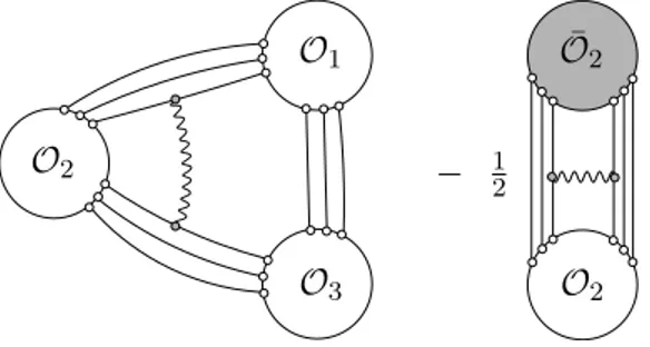
From the Feynman diagrams computation point of view, it is actually simpler to cal-culateC₁₂₃(1) instead of the combination (C₁₂₃(1) +a₁+a₂+a₃). In fact, because we have to divide by the square root of the two-point functions, all one-loop diagrams in the three-point function involving only two operators are canceled. The figure 2 has an example of a such cancellation.

The conclusion is that one is left with the computation of only genuine three-point diagrams, i.e., the diagrams involving fields from the three operators.6 The allowed posi-tions of the spin chains where it is possible to have those genuine diagrams are commonly

5_{In order to preserve the gauge invariance, one can introduce a Wilson line between the two shifted} fields. This will in principle introduce extra diagrams at one-loop, coming from the gluon emission from the Wilson line. However, we will show in the appendixDthat this additional contribution actually vanishes at this order in perturbation theory.

JHEP09(2014)173

O1

O3

O1 − 12 O2 = 0 − 1

2 O¯1 O¯2

Figure 2. The wavy-line in the figure is just a representation of a one-loop diagram (for example, a gluon exchange). When the contribution of the square root of the two-point functions is subtracted (this is the reason for the factor 1

2), all the diagrams involving just two operators are canceled.

O2

O1

O3

− 12 ¯ O2

O2

Figure 3. A genuine three-point diagram to which we subtract half of the same diagram but seen as a two-point process is shown. The constant coming from this combination of diagrams is regularization scheme and normalization independent.

called the splitting points. We are then seeking the constants coming from the genuine three-point diagrams subtracted by the constants coming from the same diagrams but now seen as two-point processes. This is exemplified in the figure 3.

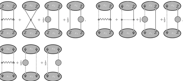
The details of the Feynman diagram computation are given in the appendix B and here we just provide the results. In the figure 4, we list all diagrams giving a non-zero contribution to the three-point functions as well as the result of the respective scheme independent constants. A relevant aspect of this computation is that some terms in the second line of (2.5) are now important at one-loop level. Indeed, from figure 4 we realize that the second graph of the second row mixes up the R-charge indices of the scalar and the fermion. In particular, the scalar Φ14 and the fermion ψ2 in the second line of (2.5) can be converted into aΨ and a ¯Z through this diagram. The resulting state can then be contracted with the remaining external operators and give a non-vanishing contribution.

From the results of figure 4, we can directly read off an operator acting on the two fields at the splitting points of an external state and that gives those same constants after contraction with the remaining states. We denote this operator by _F and define it by the following matrix elements

hψaψb_{| F |}ψcψd_i=₋δacδbd, (3.9) hΦefΦgh_{| F |}ΦabΦcd_i= 2 ¯δgh,abδ¯ef,cd₋2 ¯δef,abδ¯gh,cd₋ ǫabcdǫef gh,

JHEP09(2014)173

Figure 4. These are the relevant one-loop diagrams for the three-point functions. All other graphs give a zero contribution. The solid, wiggly and dashed lines represent the scalars, gluons and fermions, respectively. The constants are obtained by combining the three-point and two-point graphs as illustrated in figure3. We have used the point splitting regularization and the Feynman gauge. For three-point diagrams we take the limit where a pair of dots (either top or bottom) are brought to the same spacetime points. For the two-point function, both pairs of dots (top and bottom) are brought to the same spacetime points. We are using the definition ¯δab

cd ≡δ a cδ

b d−δ

b cδ

a d.

hΦdeψf_{| F |}ψcΦab_i=δceδ¯ab,df, _hψfΦde_{| F |}Φabψc_i=δceδ¯ab,df,

where ¯δab,cd_≡δacδbd₋δadδbcand in the second line we recognize theso(6) Hamiltonian [6, 7,20]. It is simple to check that the operator g₂2F reproduces the constants of figure4.

For the specific setup that we are considering only the diagrams of figure4are relevant, since additional diagrams either cancel among them or vanish, see appendix Bfor details. In the case of a more general setup, the operator _F defined receives corrections from new diagrams.

In what follows, the operator _F will appear with additional indices as _Fij, which

indicate the sites in the spin chain where the operator acts. As an example, we have that

h. . .Ψi

j

Z . . . |g 2

2Fij|. . .

i

Ψ

j

Z . . .i=−g 2

2 ,

which reproduces the result of the first diagram of the second row of figure4. It is important to note that when the operatorFij acts on non-neighboring sites, it can pick up additional

minus signs due to statistics, for example,

hΨ . . . Ψ . . . Ψ | {z }

nfermions

. . . Z_|g 2

2 F1L|Z . . . Ψ . . . Ψ| {z }

nfermions

. . . Ψ_i= (₋1)ng 2

2 ,

JHEP09(2014)173

3.3 Final result

We now give the complete expression for the structure constants up to one-loop in the setup considered in this work. It reads

C123 = α×

h1f_|1 +g 2

2FL3−N3,L3−N3+1+

g2

2 FL1,1|Z . . .¯ Z¯ | {z }

L3−N3

i1. . . iL2−N3i (3.10)

hΨ . . .¯ Ψ¯ | {z }

N3

i1. . . iL2−N3|1 +

g2

2FN3,N3+1+

g2

2FL2,1|2i

×

×hΨ . . . Ψ | {z }

N3

¯ Z . . .Z¯ | {z }

L3−N3

|1 +g 2

2FN3,N3+1+

g2

2FL3,1|3i, where we have that

α = r

L₁L₂L₃

N(1)_N(2)_N(3) , (3.11)

with_N(i) _{being the respective norms and we are using the conventions} hσi1σi2· · ·σiL|σj1σj2· · ·σjLi=δi1j1δi2j2· · ·δiLjL, whereσ is any field.

In the formula (3.10), ia can be either ¯Z or ¯Ψ and a sum over all these intermediate

states is implied. Moreover, we have included a superscriptf in the bra associated to the operator_O1to emphasize that the state wasflipped,7see [4] for details. The external states are the two-loop corrected Bethe eigenstates as described in section 3.1, for instance

|1i=|1i(0)+g2_|1i(1)+O(g4). (3.12)

We have checked that for the simple case of three half-BPS operators, the one-loop correction to the structure constant vanishes as expected from the non-renormalization theorem of [21], see appendixCfor details. Additionally, in the appendixEwe check that this result satisfies some constraints from symmetry considerations.

The expression (3.10) can now be evaluated as an explicit function of the Bethe roots by using the known form of the two-loop Bethe states. As the number of excitations of the external states increases, such task becomes tedious and the result gets lengthy obscuring possible simplifications. Nevertheless, we can easily deal with states of arbitrary length but only a few magnons. It turns out that the manipulation of the resulting expressions for these simple cases reveals a strikingly compact structure that can be easily generalizable for arbitrary complicated states. We then resort to the numerical approach in order to confirm that such generalization actually holds. In the end, we find a formula given by a

JHEP09(2014)173

C123 =C 3 Q

k=1

N_Qk

i<j

f(y_i(k), y(_jk))

N1 Q i=1 N2 Q j=1

f(y_i(1), y_j(2))

N1

Y

k=1

"

1₋(y(1)_k )L2

N2

Y

i=1

−S(y_i(2), y_k(1)) #

, (3.13)

where we are using the notationy_k(i)=eip(i)_{k and the normalization factor C is given by}

C= r

L1L2L3 N(1)_N(2)_N(3)

"

1 +g2 N₃2₋1₋1 4 3 X i=1 γi # , (3.14)

with γi being the anomalous dimension of the operator Oi. As described in the

subsec-tion 3.1, the normsN(i) _{are given by the formula} N(i)_{= det}

j,k≤Ni

∂

∂p(_ji) 

Lp(_ki)+ 1 i

Ni

X

m6=k

logS(p(_mi), p(_ki)) 

 . (3.15)

The most important and non-trivial part of the final result is the functionf which reads

f(s, t) = (s₋t)

1₋g 2 2 s t + t s − 1 s−s−

1

t −t+ 2

. (3.16)

The momentap(_kj)of the fermionic excitations must satisfy the Bethe equations which take the form

eip(j)k Lj ₌

N

Y

i6=k

−S(p(_kj), p(_ij)), (3.17) and the total momentum condition (2.16). This constitutes the most important result of this paper and it will be discussed in the next section.

4 Discussion and open problems

In this work, we have computed both the leading order contribution and the one-loop per-turbative correction at weak coupling to the three-point functions of single-trace operators ofN = 4 SYM in thesu(1|1) sector. Thesu(1|1) sector is closed to all orders in perturba-tion theory [19] and it is the simplest sector having both fermions and bosons. Representing each operator by a Bethe eigenstate, we were able to derive a simple expression (2.25) for the leading order result in terms of the momenta characterizing the states.

In addition, we have also computed the one-loop correction by evaluating the relevant Feynman diagrams and also determining the two-loop Bethe eigenstates and their norm. The prescription for computing the scheme independent three-point structure constant turns out to be given in terms of the insertion of the operator _F, defined in (3.9), at the splitting points of the spin chains.

JHEP09(2014)173

have a very simple expression for an arbitrary number of magnons, see (3.5). The norm of these states is compactly given by a simple determinant, analogous to the well known case of the su(2) sector.

The one-loop structure constant in our setup turns out to be given by the simple formula (3.13) in terms of the Bethe roots. It is tempting to investigate the thermodynamic limit of our result, namely when we consider one or more long spin chains Li ≫1, with a

large number of excitationsNi =O(Li). This might be useful for future comparison with

string theory calculations in a specific limit. An obvious open problem is the computation of the three-point functions in higher rank sectors at least at tree-level. Our result and the results of [5,10] are encouraging in order to find a simple expression for the fullpsu(2,2_|4). The main obstacle is the knowledge of the scalar products of Bethe states for generic (super) algebras, although some progress has been made in thesu(3) case [22–25].

The final expression (3.13) is very suggestive and deserves further comments. Apart from the simple normalization factor _C given by the expression (3.14), the structure con-stant has two distinct contributions. Firstly, the two-loop correction to the S-matrix ap-pears in a very natural way when we look at the tree-level result (2.25). Secondly, the most non-trivial part comes from the function f. The one-loop result is achieved by deforming this function, which bears some similarities to thesu(2) andsl(2) cases [8,10]. As already pointed out in [10], it would be interesting to deepen the connection of the three-point function with form factors as started in [26,27]. In particular, that could shed light on a (non-perturbative) definition of the function ffrom the form factors axioms. In fact, such axiomatic approach was recently explored in the context of the scattering amplitudes [28– 30]. There, the central object called pentagon transition P(u_|v) was required to satisfy some natural constraints from the integrability point of view. These conditions were then used to bootstrap the function exactly. In this regard, we notice some striking similarities of the dependence of our final result on this functionfwith the expression (9) of [28] which corresponds to a multi-particle transition. We hope that such ideas can be applied for the calculation of three-point functions at any value of the coupling constant.

Acknowledgments

We would like to thank P. Vieira for many invaluable discussions and suggestions. We also thank B. Basso, N. Berkovits, N. Gromov, Y. Jiang, H. Nastase, J. Penedones, D. Serban, A. Sever, C. Sieg, E. Sobko, J. Toledo for comments and discussions and especially T. Wang for collaboration in a stage of this project. We would like to thank the warm hospitality of the ICTP-SAIFR, FAPESP grant 2011/11973-4, where part of this work was done. TF would like to thank the warm hospitality of the Perimeter Institute where this work was initiated.

JHEP09(2014)173

F´ısica do Porto is partially funded by FCT under grant PEst-OE/FIS/UI0044/2011. TF would like to thank FAPESP grant 2013/12416-7 and 2009/50775-3 for financial support.

A Notation and conventions

In this appendix, we fix our conventions for the perturbative computations. The N = 4 SYM with SU(N) gauge group has the following Lagrangian [31,32]

L = Tr

−1₂FµνFµν+ 2DµΦabDµΦab+ 2iψαaσαµα˙(Dµψ¯a)˙

α _(A.1)

+2g_YM2 [Φab, Φcd][Φab, Φcd]−2

√ 2gYM

[ψαa, Φab]ψbα−[ ¯ψαa˙ , Φab] ¯ψαb˙

,

with all the fields in the adjoint representation of the gauge group and the covariant deriva-tive is _Dµ·=∂µ−igY M[Aµ,·]. The propagators extracted from this Lagrangian are (we

are suppressing the gauge indices and taking the leading order in N)

hΦab(x)Φcd(0)i =

¯ δ_cdab

8

1

(2π)2_(−x2_+iǫ),

hψa_α(x) ¯ψ_{β b}˙ (0)i = i δa_b

2 σ

µ

αβ˙∂µ

1

(2π)2_(−x2_+iǫ),

hAµ(x)Aν(0)i =−

ηµν

2

1

(2π)2_(−x2_+iǫ),

where ¯δ_cdab_≡δ_caδ_db₋δb_cδa_d. We are using the Minkowski metric (+_{− − −}) and the Feynman gauge. The action of the (classical) supersymmetry generators are given by [33]

[Qα_a, Φbc] = i √

2 2

δb_aψαc₋δ_acψαb, [Qαa, ψβb] = δabFβα,

[Qα_a,ψ¯_bβ˙] = 2√2Dβα˙ _Φ

ab,

and the conjugate expressions for the action of ¯Qa

˙

α. The action of the R-symmetry

generators is given by

[Rab, Φcd] = δbcΦad+δdbΦca−

1 2δ

a

b Φcd,

[Rab, ψc] = δbcψa−

1 4δ

a

b ψc.

In the computations of the Feynman diagrams, in particular for the evaluation of the integrals, we analytical continued to Euclidean space by using

x0 =ix4, σ0_M =−σ0_E, σ_Mi =iσ_Ei ,

where the subscriptsM means Minkowski space andE means Euclidean space,

JHEP09(2014)173

Figure 5. The results of the Feynman diagrams computation omitting both terms that must vanish or cancel when summing all the diagrams (see text) and factors ofN. The solid, wiggly and dashed lines represent the scalars, gluons and fermions, respectively. The ¯δwas defined in appendix A.

B One-loop perturbative computation details

In this appendix, we present the details of the perturbative computation of the three-point functions at one-loop using the point splitting regularization. As reviewed in the main part of this paper, in order to obtain scheme and normalization independent structure constants we also need to know the results of the two-point functions. For completeness, we explicitly compute the one-loop dilatation operator of the su(1|1) sector as well.

Typically three kinds of integrals will appear in the computations

Y₁₂₃ = Z

d4u Ix1uIx2uIx3u,

X1234 = Z

d4u Ix1uIx2uIx3uIx4u,

H12,34 = Z

JHEP09(2014)173

Ixaxb ≡

1 (2π)2_(xa−x

b)2

.

The Y and X integrals are well-known and explicit expressions for them can be found for instance in [7,34]. The integralH is not known analytic, however, only its derivatives will be needed. In particular, the following combination [34] turns out to be useful

F₁₂,34 ≡

(∂1−∂2)·(∂3−∂4)H12,34 Ix1x2Ix3x4

(B.1)

= X1234 Ix1x3Ix2x4

−_I X1234

x1x4Ix2x3

+G1,34−G2,34+G3,12−G4,12, where

Ga,bc =

Yabc

Ixaxc

−_IYabc

xaxb

.

We will need several limits of the expressions for Y and X, namely when pairs of distinct points collapse into each other

Y113 ≡ lim

x2→x1

Y123 =

2₋log

ǫ2 x2₁₃

Ix1x3 16π2 ,

X1134 ≡ lim

x2→x1

X1234 =

2₋log

ǫ2x2₃₄ x2₁₃x2₁₄

Ix1x3Ix1x4 16π2 ,

where we are considering xµ₂ = xµ₁ +ǫµ with ǫµ _→ 0. We can also take a further limit of the last expression above whenx4 →x3 giving

X1133=

1−log

ǫ2 x2₁₃

_I2

x1x3

8π2 .

Moreover, we also need limits of the first and second derivatives of both theY and theX integrals. We include the results of them below for completeness. The first derivatives are given by

lim

x2→x1

∂₁,µY123 = ǫµ

ǫ2 Ix1x3

8π2 −

1−log _ǫ2

x2_{13 x}

13,µIx21x3

4 −

x13,νǫνǫµIx21x3

2ǫ2 , (B.2)

lim

x2→x1

∂3,µY123 =

1−log

ǫ2 x2₁₃

_x

13,µIx21x3

2 , (B.3)

lim

x2→x1

∂1,µX1234 = ǫµ

ǫ2

Ix1x3Ix1x4 8π2 −

1−log

ǫ2x2₃₄ x2₁₃x2₁₄

_x

13,µIx21x3Ix1x4 +x14,µIx1x3Ix21x4 4

−x14,νǫ

ν_ǫ

µIx1x3Ix21x4

2ǫ2 −

x13,νǫνǫµIx21x3Ix1x4

2ǫ2 ,

lim

x2→x1

∂3,µX1234 = −

x34,µIx1x3Ix1x4Ix3x4

2 +

1−log

ǫ2x2₃₄ x2₁₃x2₁₄

_x

13,µIx21x3Ix1x4

2 ,

As before, one can take further limits of these expressions when needed. The second derivatives read

lim

x2→x1

∂1,µ∂2,νY123 =− ǫµǫν

ǫ4 Ix1x3

4π2 +

ǫµǫνIx21x3

ǫ2

1 6+

x₁₃,ρǫρ

ǫ2 −

16π2x₁₃,ρǫρx13,σǫσIx1x3 3ǫ2

JHEP09(2014)173

ǫ2

x13,µIx21x3

2 −

ǫµ

ǫ2

x13,νIx21x3

2 +

8π2x13,ρǫρIx31x3

3ǫ2 (2x13,νǫµ−x13,µǫν) +1

ǫ2

δµνIx1x3

8π2 −δµνI 2

x1x3

11 36 +

x13,ρǫρ

2ǫ2 −

8π2x13,ρǫρx13,σǫσIx1x3 3ǫ2

+ 1 12log

_ǫ2

x2₁₃

I_x2_1x3δµν+

2π2 9

1₋6 log _ǫ2

x2₁₃

x13,µx13,νIx31x3, lim

x2→x1

∂₁,µ∂3,νY123 = ǫµǫν

ǫ2 I_x2_1x3

2 +

ǫµ

ǫ2x13,νI 2

x1x3−2π

2₁

−2 log _ǫ2

x2₁₃

x₁₃,µx13,νIx31x3 +1

4

1−log _ǫ2

x2₁₃

I_x2_1x3δµν−

8π2x₁₃,νǫµx13,ρǫρIx31x3

ǫ2 , (B.4)

lim

x2→x1

∂₁,µ∂2,νX1234 =− ǫµǫν

ǫ4

Ix1x3Ix1x4 4π2 +

ǫµǫνIx21x3I 2

x1x4

6ǫ2

1 Ix3x4

−32π 2_x

13,ρǫρx14,σǫσ

ǫ2

+ǫµǫνǫ

ρ_I

x1x3Ix1x4

ǫ4 (x14,ρIx1x4 +x13,ρIx1x3) −16π

2_ǫ

µǫνǫρǫσIx1x3Ix1x4

3ǫ4 (x14,ρx14,σI 2

x1x4 +x13,ρx13,σI

2

x1x3)

−ǫµIx1x3Ix1x4

2ǫ2 (x14,νIx1x4 +x13,νIx1x3) +ǫνIx1x3Ix1x4

2ǫ2 (x14,µIx1x4 +x13,µIx1x3) +8π

2_ǫ

µǫρIx1x3Ix1x4

3ǫ2 ( 2x14,νx14,ρI 2

x1x4 +x13,ρx14,νIx1x3Ix1x4)

+8π 2_ǫ

µǫρIx1x3Ix1x4

3ǫ2 ( 2x13,νx13,ρI 2

x1x3 +x14,ρx13,νIx1x3Ix1x4)

−4π 2_ǫ

νǫρIx1x3Ix1x4

3ǫ2 ( 2x14,µx14,ρI 2

x1x4+x13,ρx14,µIx1x3Ix1x4)

−4π 2_ǫ

νǫρIx1x3Ix1x4

3ǫ2 ( 2x13,µx13,ρI 2

x1x3+x14,ρx13,µIx1x3Ix1x4)

+1 ǫ2

Ix1x3Ix1x4δµν 8π2 −

Ix1x3Ix1x4δµν

4 (Ix1x4 +Ix1x3) −Ix1x3Ix1x4δµνǫρ

2ǫ2 (x14,ρIx1x4+x13,ρIx1x3) +8π

2_I

x1x3Ix1x4δµνǫρǫσ

3ǫ2 (x14,ρx14,σI 2

x1x4 +x13,ρx13,σI

2

x1x3)

+8π 2_I

x1x3Ix1x4δµνǫρǫσ

3ǫ2 x13,ρx14,σIx1x3Ix1x4 + 1

36

−2 + 3 log _ǫ2_x2

34 x2₁₃x2₁₄

_I2

x1x3I

2

x1x4δµν

Ix3x4 +2π

2

9

1−6 log _ǫ2_x2

34 x2₁₃x2₁₄

x₁₃,µx13,νIx31x3Ix1x4 −2π

2

9

1 + 3 log

ǫ2x2₃₄ x2₁₃x2₁₄

(x13,νx14,µ+x13,µx14,ν)Ix21x3I 2

x1x4

+2π 2

9

1−6 log

ǫ2x2₃₄ x2₁₃x2₁₄

x14,µx14,νIx1x3I 3

JHEP09(2014)173

Figure 6. The results of the Feynman diagrams for the two-point functions. They are obtained by taking the limitsx3→x2 andx4→x1 of the expressions in figure5.

lim

x2→x1

∂₁,µ∂3,νX1234 = ǫµǫν

ǫ2

I_x2_1x3Ix1x4 2 + 2π

2_log ǫ2x234 x2₁₃x2₁₄

x₁₃,νx14,µIx21x3I 2

x1x4

+x13,νǫµI 2

x1x3Ix1x4

ǫ2 ( 1−4π 2_x

14,ρǫρIx1x4−8π 2_x

13,ρǫρIx1x3) +2π2

−1 + 2 log

ǫ2x2₃₄ x2₁₃x2₁₄

x13,µx13,νIx31x3Ix1x4 −1

4

−1 + log

ǫ2x2₃₄ x2₁₃x2₁₄

I_x2_1x3Ix1x4δµ,ν +2π2x13,µx34,νIx21x3Ix1x4Ix3x4+ 2π

2_x

14,µx34,νIx1x3I 2

x1x4Ix3x4,

lim

x2→x1

∂3,µ∂4,νX1234 = δµν

2 Ix1x3Ix1x4Ix3x4−4π 2_x

34,µx34,νIx1x3Ix1x4I 2

x3x4

−4π2x14,νx34,µIx1x3I 2

x1x4Ix3x4 + 4π

2_x

13,µx34,νIx21x3Ix1x4Ix3x4 −4π2x13,µx14,ν log

ǫ2x2₃₄ x2₁₃x2₁₄

I_x2_1x3I_x2_1x4.

Using the above results, we can proceed to the computation of the two- and three-point functions. The result of all the non-zero Feynman diagrams relevant for us is given in figure 5, where we have omitted terms involving ǫµνρλ that must either vanish when a pair of point collide or cancel when all the diagrams are summed. This is the case in order to preserve conformal invariance and parity.

The results of figure 5only contain derivatives of the functionH12,34and it is possible to evaluate them explicitly [35]. Consider the case when the derivatives act on either the first or the second pair of points of H, namely ∂1·∂2H12,34, and also the case when they act on a point belonging to the first pair and a point belonging to the second pair, for instance∂1·∂4H12,34. The first case is straightforward to compute by using integration by parts and the property of the euclidean propagatorxIxy =−δ(4)(x−y). The result is

∂1·∂2H12,34= 1

JHEP09(2014)173

Figure 7. Using the results of figure6, the sum of the graphs appearing in this figure gives precisely thesu(1_|1) Hamiltonian of (B.11).

For computing the second case, we need the function F12,34 defined in (B.1) and some identities ofH12,34. Firstly, note that H satisfies the equation

(∂1,µ+∂2,µ+∂3,µ+∂4,µ)H12,34= 0, (B.6) which can be proved by integration by parts. Similarly, it is possible to show that the following identity holds

∂i·∂jH12,34= 1

2(k+l−i−j)H12,34+∂k·∂lH12,34 (B.7) fori₆=j₆=k₆=l. In order to get∂1·∂4H12,34, it is convenient to write it as

∂_1·∂₄H₁₂,34= 1

2(∂1·∂3+∂1·∂4)H12,34− 1

2(∂1·∂3−∂1·∂4)H12,34. (B.8) Now using (B.7), one can show that the first term on the right-hand side of (B.8) can be written as

1

2(∂1·∂3+∂1·∂4)H12,34=− 1

2(1H12,34+∂1·∂2H12,34) (B.9) whereiH12,34can be computed using the equation defining the euclidean propagator and ∂_1·∂₂H₁₂,34 is known from (B.5). Using (B.6), the second term on the right-hand side of (B.8) can be written as

1

2(∂1·∂3−∂1·∂4)H12,34= 1

4(F12,34Ix1x2Ix3x4 + (4−3)H12,34). (B.10) Finally, substituting (B.9) and (B.10) in (B.8), one gets an expression for ∂1 ·∂4H12,34. The expressions for the remaining cases where the derivatives act on other points can be deduced analogously.

JHEP09(2014)173

work. The solid and dashed lines represent the scalars and fermions, respectively.

in figure6. Summing all the diagrams as illustrated in figure 7, one obtains the one-loop Hamiltonian operator

H = 2g2(I₋SP), (B.11)

where SP is the superpermutator which exchanges the fields and picks up a minus sign when both fields are fermionic. This Hamiltonian is the well known result of [15,19].

We now proceed to the three-point functions. In order to obtain the constant coming from each diagram, one takes the limit of the expressions given in figure 5 where a single pair of points collapses into each other. After taking that limit, the result will have constant terms, divergent logarithmic terms and eventually Y functions and their derivatives. The derivatives of theY functions can be expressed in terms of the Y function itself by using some of its properties. This will be explained in detail in the appendix C. After this procedure, the logarithmic terms will contribute to the standard regulator dependence in (3.8) and the remaining Y functions will cancel with similar contributions from other diagrams in a way that the conformal invariance is restored. One can then read the constant part of the diagram. The final step is to subtract one half the constant coming from the same diagram but when the two pairs of points collapse into each other as described in figure 3. The results are given in figure4.

Let us comment now on a detail of this computation. Our final results presented in the figures 4and 5do not contain the Feynman diagrams of figure 8. This is the case because the first two graphs of this figure turn out to cancel among them. They can give a non-zero contribution in our setup only when either b =c = 4 anda = 3 or a=c = 2 andb = 3. However, as these two graphs always appear with the same weight and opposite signs, they end up canceling. The last graph of the figure8 must vanish when |x_{12| →}0 because it is

∝ ǫγδǫγ˙δ˙σµ

Eγ˙1σ

ν

Eδ˙1σ

ρ

E1 ˙γσ

λ

E1 ˙δ

Z

d4v d4u(∂_µvIx1v)(∂

v

νIx2v)Ivu(∂

u

ρIx3u)(∂

u

λIx4u) →0.

JHEP09(2014)173

considered in (C.1)–(C.3). Note that only the first term ofO3in (C.3) gives a non-zero contribution

at this order in perturbation theory as the second term clearly gives a vanishing contribution due toR-charge conservation.

C Some examples of three-point functions

In this appendix, we give two examples of three-point functions. The first one is the case of three half-BPS operators. It is well-known that this correlator is protected and therefore it constitutes a check for our computations. Then we compute a non-protected three-point function both by brute force and by using our prescription of inserting the operator_F at the splitting points.

C.1 Three half-BPS operators

Consider the following three half-BPS operators

O1 = Tr (ZZ) , (C.1)

O2 = Tr ¯ΨZ¯ , (C.2)

O3 = (R24R13)·Tr (Ψ Z) = Tr ΨZ¯

+ Tr ψ2Φ14 . (C.3)

At tree-level the result is simply given by the sum of the two diagrams of figure9and reads

hO1(x1)O2(x2)O3(x3)i=

2 (2π)6₈2_x2

12x213

(σ_Eµ)_{1 ˙1}∂3,µ

1

2x2₂₃. (C.4)

At one-loop, one has to sum the diagrams of figure 10and use the results given in figure 5 taking the appropriate limits.

Some diagrams will still contain the functionY and its first derivatives. TheY function depends on the external points in a way that does not respect the spacetime dependence fixed by conformal symmetry, see equation (3.8). However, when one sums the different diagrams this non-conformal spacetime dependence turns out to cancel identically.

JHEP09(2014)173

Figure 10. The one-loop diagrams contributing to the three-point function of the three half-BPS operators considered in (C.1)–(C.3). In the last four diagrams of the second row, the second term of _O3 (see expression (C.3)) gives a non-zero result. In all other diagrams only the first term of

O3 contributes.

JHEP09(2014)173

opera-tors (C.5)–(C.7). Once again, we only need to consider the first term of (C.7) at this order in perturbation theory.

C.2 Two non-BPS and one half-BPS operators

We consider now a non-protected three-point function. This example serves as an illus-tration of some of the technical details of the brute force computation. Moreover, we also use it to check our prescription of the _F operator insertion at the splitting points. The operators at one-loop level that we will consider are

O1 = Tr (ZΨ Ψ Z), (C.5)

O2 = Tr ¯ZΨ¯Ψ¯Ψ¯ , (C.6)

O3 = (R24R13)·Tr (Ψ Z) = Tr ΨZ¯

+ Tr ψ2Φ14 . (C.7)

Note that the O1 and O2 are not half-BPS and therefore they will receive corrections as explained in subsection 3.1. However, to compute the Feynman diagrams contribution we do not need to take them into account. At tree-level the result is simply the sum of the two diagrams of figure12 which gives

hO1(x1)O2(x2)O3(x3)i0 =− 2 (2π)10₈2_x2

13x212

×

(σ_Eµ)_{1 ˙1}∂1,µ

1

2x2₁₂ (σ

ν

E)1 ˙1∂1,ν

1

2x2₁₂ (σ

ρ

E)1 ˙1∂3,ρ

1 2x2₂₃

.

The diagrams contributing at one-loop are represented in figure 13.

As in the previous example, the dependence of each diagram on the Y function and its derivatives will cancel when we sum over all the diagrams. This ensures that we obtain a conformal invariant result. However, this cancellation is not immediate and it relies on several properties of theY function. The first observation is that the functionY is given by

Y123=

π2φ(r, s)

(2π)4 Ix1,x3, (C.8)

where r = x212

x2₁₃ and s =

x2

23

x2₁₃ and an explicit expression for φ(r, s) can be found in [34].

The important information for us is that the function φsatisfies the following differential equations [7]

φ(r, s) + (s+r₋1)∂sφ(r, s) + 2r∂rφ(r, s) = −

logr

JHEP09(2014)173

JHEP09(2014)173

Figure 14. Inserting the operator _F at the splitting points reproduce the result of the one-loop Feynman diagrams.

φ(r, s) + (s+r₋1)∂rφ(r, s) + 2s∂sφ(r, s) = −

logs r ,

which can be used to relate the first derivatives of Y with Y itself. In addition, one can take derivatives with respect tor and sof both the equations above to arrive at a system of equations that relates second derivatives of φ with first derivatives and the function φ itself. Using then (C.8), it is trivial to get rid of the second derivatives of Y. These properties of the function φ ensure that the non-conformal dependence of the three-point function indeed cancel when all diagrams are summed over.

The final result is given by

hO1(x1)O2(x2)O3(x3)i=hO1O2O3i0

1 + 4g2

−1 + 2 log

ǫ2 x2₁₂

+_O(g4)

,

which comparing with (3.8) gives the correct anomalous dimensions of the operators. This is a non-trivial consistency check of our computation.

JHEP09(2014)173

Figure 16. The Wilson line contributions to the two-point functions. In the combination of the two- and the three-point diagrams that provide the scheme independent structure constant C₁₂₃(1)

of (3.8), all the extra diagrams coming from the Wilson lines cancel each other at this order in perturbation theory. In the figure, the diagram corresponding to the emission of a gluon between the two Wilson lines is not depicted, since it is proportional toǫ2 _{and vanishes in the limitǫ→0.}

the one-loop constant. We obtain the following contribution from the Feynman diagrams to the structure constant

C₁₂₃(1)

Feynman diagrams contribution =₋3

2. (C.10)

Recall that this is not the final result, one also has to add the extra contribution from the corrected two-loop Bethe states.

Finally, it is possible to test our prescription of inserting the _F operator at the split-ting points, see figure 14. Summing over all these insertions gives precisely the contribu-tion (C.10) to the structure constant.

D Wilson line contribution

JHEP09(2014)173

D.1 Wilson line connecting two scalars

In our conventions the Wilson line operator is defined by

Wl=Pexp

i gY M

Z

Aµd~xµ

.

When inserting a Wilson line connecting two scalars, it is necessary to consider the one-loop graphs corresponding to the gluon emission depicted in figure 15(a). Let us define ǫµ = xµ₄₋xµ₃ and at the end of the day we will take the limit ǫµ_→0. Then we can conveniently parametrize the Wilson line byxµ(z) =xµ₃+zǫµ. The result of the sum of the diagrams is

figure15(a) = λ 128

Z 1

0

dz ǫµ(Ix2x3∂

µ

1 Y1x4−Ix1x4∂

µ

2 Y2x3+Ix1x4∂

µ

3 Y2x3−Ix2x3∂

µ

4 Y1x4), (D.1) where we have suppressed both theR-charge and the gauge indices which are the same as in the tree-level case. From the formula (B.3), it follows that the first and second terms of the above result are of orderǫand therefore vanish in the limitǫ_→0. However, from (B.2) we see that the third and last term give a finite contribution.

In order to compute the scheme and normalization structure constant C₁₂₃(1) of (3.8), we have to subtract from the previous result one half of the one-loop diagrams from the two-point functions as shown in figure16 (we take both the limitsx4 →x3 and x2 →x1). It is simple to show that the contribution of these diagrams cancels exactly the constant coming from the expression (D.1). So, at this order in perturbation theory we do not get any further contribution toC₁₂₃(1) and therefore we can safely ignore the Wilson lines.

D.2 Wilson line connecting either a scalar and a fermion or two fermions

In the case of a scalar and a fermion connected by a Wilson line, the contribution of the diagrams depicted in 15(b) is given by

figure 15(b) = λ 32

Z 1

0

dz ǫµhIx2x3(σEµ1 ˙1∂4·∂1Y1x4−σ_Eν_{1 ˙1}∂ν4∂µ1Y1x4−σ_Eν_{1 ˙1}∂µ4∂ν1Y1x4 −ǫρµλνσ_Eν_{1 ˙1}∂4,λ∂1,ρY1x4) +σ_Eν_{1 ˙1}∂ν1Ix1x4(∂

3

µY2x3−∂µ2Y2x3)

i

. (D.2)

Using the expressions (B.2)–(B.4), one can easily see that this gives a finite contribution in the limit when ǫ goes to zero (in particular, the term with ǫρµλν vanishes). To this

result, we have again to subtract one half of the one-loop diagrams from the two-point functions as was done in the previous subsection for the case of two scalars. Once again, the contribution of these diagrams cancels exactly the expression (D.2).

In the case when we have a Wilson line connecting two fermions, the same argument holds. Hence at one-loop level, we can ignore the Wilson lines contributions in all cases.

E A note on the su(1|1) invariance of the final result

JHEP09(2014)173

in (3.10) when g _→ 0. One possible way of implementing a symmetry transformation on a state at any value of the coupling is to add a Bethe root with zero-momentum. It is clear from the Bethe equations that we obtain a state with the same energy and therefore belonging to the same multiplet as the original one. Consider then the states |1i and |2i with one of their momentap(1)_j andp(2)_i being equal to zero. In this particular case, we can write apart from possible signs

|2_i= ¯Q|2,_{pˆ(2)_{i }i}, _h1f_|= _h1f,_{pˆ(1)_{j }|}S¯,

where the hat over a p means that this momentum is absent. The operator ¯Q ( ¯S) cre-ates (annihilcre-ates) a momentum magnon on a ket and annihilcre-ates (crecre-ates) a zero-momentum magnon on the bra (we are omitting the R-charge and Lorentz indices for simplicity).

For this particular choice of momenta the expression (3.10) for g= 0 becomes

h1f,_{pˆ_j(1)_}|S¯ O˜3 Q¯ |2,{pˆ(2)i }i=h1f,{pˆ

(1)

j }|O˜3 {S¯,Q¯} |2,{pˆ

(2)

i }i, (E.1)

where we denote the operator _|Z . . .¯ Zi¯ 1. . . iL2−N3ihΨ . . .¯ Ψ i¯ 1. . . iL2−N3| by ˜O3. Moreover in this equality, we have used that ¯Sand ˜O3 commute which can be proved by applying the commutator to a generic su(1_|1) state. In addition, we have also used that

¯

S_|2,_{pˆ(2)_{i }i}= 0, (E.2) as the state is primary.

Now, the anticommutator _{S¯,Q¯}is given by (see for instance the appendix D of [36])

{S¯,Q¯_}=_L+ 1

2H(g), (E.3)

whereLis the length operator andH(g) is the Hamiltonian operator. When acting on the state|2,_{pˆ(2)_{i }i}it gives at leading order the length of the state L₂. In conclusion, we have derived the following equality

| h1f_|O˜3|2i |=L2| h1f,{pˆ(1)j }|O˜3|2,{pˆ

(2)

i }i |. (E.4)

The relation above shows how the structure constant changes under su(1_|1) transfor-mations of the states _|2_i and _h1f_{| at leading order. It is now simple to check that our}

expression for this scalar product given in the main text indeed satisfies this relation. At one-loop, the final expression for the structure constants given in (3.10) has the following term

h1f_|O˜′_3|2_i, (E.5)

where

˜ O3′ =

1 +g

2

2 FL3−N3,L3−N3+1+

g2 2 FL1,1

˜ O3

1 +g

2

2 FN3,N3+1+

g2 2 FL2,1