J. Braz. Comp. Soc. vol.12 número4

(1)

Concurrent Blind Channel

Equalization with Phase

Transmittance RBF Neural

Networks

Diego Vier Loss

1

, Maria C. F. De Castro

1

, Paulo Roberto Girardello Franco

1

&

Fernando C. C. de Castro

1

1_{Department of Electrical Engineering} Wireless Technologies Research Center - CPTW Pontifical Catholic University of Rio Grande do Sul

Av. Ipiranga 6681 Phone: +55 (51) 33203500 sn: 4403 Zip 90619-000 – Porto Alegre - RS - BRAZIL

fabio.dagostini@pucrs.br—sirlesio.carboni@pucrs.br—cristinacastro@pucrs.br—fcastro@pucrs.br

Abstract

This paper presents a new complex valued radial basis function (RBF) neural network (NN) with phase transmittance between the input nodes and output, which makes it suitable for channel equalization on quadrature digital modulation systems. The new Phase Transmittance RBFNN (PTRBFNN) differs from the classical complex valued RBFNN in that it does not strictly rely on the Euclidean distance between the input vector and the center vectors, thus enabling the transference of phase information from input to output. In the context of blind channel equalization, results have shown that the PTRBFNN not only solves the phase uncertainty of the classical complex valued RBFNN but also presents a faster convergence rate.comes the abstract of the paper.

Keywords: Neural Network, Equalizer, Phase, Concurrent, Blind

1. I

NTRODUCTION

Several complex valued RBF neural network approaches has been proposed in the context of channel equalization [1]-[5]. These classical approaches share a common architecture, shown in Figure 1, and a common principle – the output of the kth Gaussian center

ϕ

_k is based on the Euclidean

norm between the complex valued input vector

u

and

the kth center vector

Ψ

_k, as given by (1)

( )

_⎟⎟

⎠

⎞

⎜⎜

⎝

⎛

Ψ

−

=

exp

1

₂ _k 2

k

u

σ

ϕ

(1)

where

u

=

[

u

0

u

1

L

u

_L−1

]

T is the vector

(2)

such that

Z

{ }

u

l

=

Z

{ }

u

l₋₁

z

−1,i.e., the channel

regressor behaves as a FIFO [6].

Z

{}

⋅

is the operator which returns the Z-Transform of its argument, with

1 ,

,

2 ,

1 −

=

L

l

_.

k

Ψ is the kth center vector

[

]

T

L1 1

0 −

=

ψ

L

_, 2

k

σ

is the variance of the kth Gaussian center,

k

=

0 ,

1 ,

L

,

K

−

1

_{, being}

_K

_the

adopted number of centers.

⋅

is the operator which returns the Euclidean norm of its argument.

Figure 1: RBF neural network architecture.

From Figure 1 the output is

∑

−

=

⋅

=

1

0

K

k

k k T

W

y

ϕ

(2)

where

W

_k is the kth complex valued component of the output synapses vector

[

]

T

K

W W

W

W= 0 1 L −1 and

ϕ

k is the kth real valued

component of the hidden layer output vector

[

]

T

K1 1

0 −

=

ϕ

L

_.

In digital communications using quadrature modulation, the information is conveyed across the channel by means of a discrete sequence

s

( )

n

of complex numbers

I

+

jQ

, each complex number

being denoted as an IQ symbol of the sequence

s

( )

n

[6]. This sequence is generated by the digital transmitter at the specific symbol rate

S

_R of the system, which defines the time interval

T

between IQ symbols

s

( )

n

and

s

(

n

+

1 )

as

T

=

1 S

_R, being

L

,

1 ,

0 =

n

.

The digital modulator at the transmitter maps each incoming binary word of fixed length into the respective IQ symbol. Since an IQ symbol is a complex phasor, the phase of each IQ symbol plays a crucial role in the information flow.

Subsequently, the transmitted IQ symbol sequence

( )

n

s

is convolved with the discrete complex valued impulse response of the communication channel, impulse response which is dictated by the channel multipath scenario [6]. This multipath scenario imposes phase and amplitude distortions to

s

( )

n

. In addition, besides the multipath distortion, the channel adds noise to

s

( )

n

, so that the received sequence

( )

n

r

barely resembles the original transmitted

sequence

s

( )

n

.

At the digital receiver, the received IQ sequence

( )

n

r

is stored in the FIFO buffer of the channel

regressor

u

, so that an equalizer can perform the so called channel deconvolution process [9]. Once

r

( )

n

is deconvolved by the equalizer, the digital demodulator de-maps each deconvolved IQ symbol into the respective binary word of fixed length and of duration

T

[6].

Notice from (1) and (2) that the phase of the input

u

is not explicitly transmitted to the output

y

, since it is discarded by the Euclidean norm operator in (1). Therefore, the resulting hidden layer output vector

ϕ

restricts the RBFNN forward transmittance to be real valued, which inherently imposes some restrictions when the classical RBFNN is applied to blind channel equalization, since the forward transmittance does not explicitly convey any phase information.

In order to avoid the explicit phase invariance on the transmittance function of the classical RBFNN network we propose a new complex valued RBFNN – the Phase Transmittance RBFNN (PTRBFNN). Specifically, we replace the Euclidean norm based hidden-layer radial basis function by the complex valued basis function

( )

_{{ }}

{ }

⎟⎟ ⎠ ⎞ ⎜⎜

⎝ ⎛

Ψ − −

⋅ +

⎟⎟ ⎠ ⎞ ⎜⎜

⎝ ⎛

Ψ − −

=

2

2 2

Im Im Im

1 exp

Re Re Re

1 exp

k k

k

u j

u u

σ σ ϕ

(3)

Notice that this approach turns phase-sensitive the hidden neurons input-output relationship while preserving the locality of the basis function.

Notice also that

σ

_k2

=

Re

{ }

σ

_k2

+

j

Im

{ }

σ

_k2 does not strictly imply a complex valued physical interpretation for the variance of the kth complex valued center

ϕ

_k.

{ }

2

Re

σ

_k is just a quadratic measure for the reach radius of the basis function Re

{ }

ϕ

_k . Likewise, same interpretation apply to

Im

{ }

σ

_k2 with respect to

{ }

ϕ

k

Im

.

2. T

HE PTRBFNN LEARNING ALGORITHM

Let

u

( )

n

be the channel regressor at the instant

n

, and let

d

( )

n

be the desired complex value at the PTRBFNN output y

( )

n . In the context of channel equalization, d

( )

n is the original transmitted IQ symbol training sequence whose values are stored in a look up table at the receiver as reference data for the learning process. Actually, as we shall see further, the reference IQ symbol training sequence for the RBFNN learning process is based on a blind concurrent algorithm. For now, lets just assume d

( )

n is known at the receiver.

In this work we adopt a gradient based learning process. It consists of , for each received IQ symbol at the instant

n

, to adjust by means of the Delta Rule [8] the PTRBFNN free parameters

Ψ

_k,

σ

_k2 and

W

,

1 ,

,

1 ,

0 −

=

K

k

L

_{, so that after a sufficient number}

of received IQ symbols the distance between

y

( )

n

and

d

( )

n

is as close as possible to zero. A quadratic measure of the distance between

y

( )

n

and

d

( )

n

is:

( )

2

1 n

y

n

d

n

J

=

−

(4)

Specifically, the learning process consists of to minimize the cost function given by (4) by adjusting the PTRBFNN free parameters

W

( )

n

,

Ψ

k

( )

n

and

( )

n

k 2

σ

at each instant

n

[8]. For any PTRBFNN free parameter

℘

, the Delta Rule adjusts

℘

according to:

(

n

+

)

=

℘

n

−

∇

J

( )

n

℘

1 (

)

η

(5)

where

η

is the learning rate or adaptation step [7][8] and

∇

J

is the gradient of the cost function

J

with respect to the parameter

℘

:

( )

n

J

n

J

∂℘

∂

=

∇

(6)

Let

W

p be the th

p

component of vector

[

]

T

K

W

=

₀ ₁

L

₋₁ .

W

_p is one of the PTRBFNN free parameters which is adjusted by (5), so that

(

n

)

W

( )

n

J

( )

n

W

p W p

p

+

1 =

−

η

∇

(7)

where

η

_W is the adaptation step and

{ }

p

{ }

p

p W

p

W

J

j

W

J

W

J

Im

Re

∂

+

∂

=

∂

=

∇

(8)

For convenience, in the equations that follow we drop

n

from the notation, unless its presence is strictly necessary. From (2) and (4) the real and imaginary parts of (8) are obtained as

{ }

p

{ }

p p

K

k

k k

p p

e

W

d

W

y

d

W

J

ϕ

Im

Re

2

1 Re

2

1 Re

2 1

0

2

−

=

∂

−

∂

=

∂

−

∂

=

∂

∑

−

=

(9)

{ }

p

{ }

p p

K

k

k k

p p

e

W

d

W

y

d

W

J

ϕ

Im

Re

Im

2

1 Im

2

1 Im

2 1

0

2

+

−

=

∂

−

∂

=

∂

−

∂

=

∂

∑

−

=

(10)

where

e

=

d

−

y

is the learning process instantaneous error.

(4)

(

n

)

W

( )

n

e

( ) ( )

n

W

+

1 =

+

η

_W

ϕ

*

(11)

where

{}

⋅

∗denotes the complex conjugate operator.

Likewise, let

Ψ

_pq be the

q

th component of the th

p

center vector

[

]

T

pL pq

p p

p = Ψ 0 Ψ1 Ψ Ψ −1

Ψ L L ,

1 ,

,

1 ,

0 ⋅

⋅

−

=

L

q

and

p

=

0 ,

1 ,

⋅

,

K

−

1

.

Ψ

_pq is also a PTRBFNN free parameter which is adjusted by (5), so that

(

n

)

pq

( )

n

J

pq

( )

n

pq Ψ Ψ

∇

−

Ψ

=

+

Ψ

1 η

(12)

where

η

_Ψ is the adaptation step and

{ }

pq

{ }

pq

pq pq

J

j

J

Ψ

∂

+

Ψ

∂

=

Ψ

∂

=

∇

Ψ

Im

Re

(13)

From (2) and (4) the real and imaginary parts of (13) are obtained as

{ }

_{{ }}

{ }

[

{ }

W { }e

{ }

W { }e

]

u W d y d J p p p p p pq K i i i pq pq Im Im Re Re Re Re Re Re 2 Re 2 1 Re 2 1 Re 2 2 1 0 2

]

[

+ Ψ − − = Ψ ∂ − ∂ = Ψ ∂ − ∂ = Ψ ∂ ∂

∑

− = σ ϕ ϕ

(14)

{ }

_{{ }}

{ }

[

{ }

W

{ }

e

{ }

W

{ }

e

]

u W d y d J p p p p p pq K i i i pq pq Re Im Im Re Im Im Im Im 2 Im 2 1 Im 2 1 Im 2 2 1 0 2

]

[

− Ψ − − = Ψ ∂ − ∂ = Ψ ∂ − ∂ = Ψ ∂ ∂

∑

− = σ ϕ ϕ

(15)

From (14), (15), (13), (12) and in vector representation: ( ) ( ) ( )

{

}

{( )}

_{

{

_}

( )

}

( ) ( ) ( )

[

]

( )

{

}

{( )}

{

( )

}

( )

{

}

( ) ( ) ( ) ( )

[

]

⎪⎪ ⎪ ⎪ ⎭ ⎪ ⎪ ⎪ ⎪ ⎬ ⎫ ⎪ ⎪ ⎪ ⎪ ⎩ ⎪ ⎪ ⎪ ⎪ ⎨ ⎧ − ⋅ Ψ − − + ⋅ Ψ − ⋅ + Ψ = + Ψ ∗ ∗ ∗ ∗ Ψ n e n W n e n W n n n u n n e n W n e n W n n n u n n n p p p p p p p p p p p p 2 2 Im Im Im Im ) ( ) ( Re Re Re Re 1

]

[

]

[

σ ϕ σ ϕ η

(16)

The last PTRBFNN free parameter which is adjusted by (5) is the

p

th center variance

σ

_p2. Thus, from (5),

(

n

)

_p

( )

n

J

_p

( )

n

p

σ σ

η

σ

2

+

₁

=

2

−

∇

(17)

where

η

_σ is the adaptation step and

{ }

2

{ }

2

Im

Re p p

p p J j J J J

σ

σ ∂ ∂ + ∂ ∂ = ∂ ∂ = ∇

(18)

From (2) and (4) the real and imaginary parts of (18) are obtained as

{ }

(

)

[

{ }

W { }e

{ }

W { }e

]

u W d y d J p p p p p p K i i i p p Im Im Re Re Re Re Re Re Re 2 1 Re 2 1 Re 2 2 2 2 2 1 0 2 2 2 + Ψ − − = ∂ − ∂ = ∂ − ∂ = ∂ ∂

∑

− = σ ϕ σ ϕ σ σ

(19)

{ }

(

)

[

{ }

W { }e

{ }

W { }e

]

u W d y d J p p p p p p K i i i p p Re Im Im Re Im Im Im Im Im 2 1 Im 2 1 Im 2 2 2 2 2 1 0 2 2 2 − Ψ − − = ∂ − ∂ = ∂ − ∂ = ∂ ∂

∑

− = σ ϕ σ ϕ σ σ

(20)

From (19), (20), (18) and (17):

( ) ( ) ( ) { }

{

( )

}

{

( )

}

( )

{

}

(

)

( )

{

}

{( )}

{

( )

}

{( )}

[

]

( ) { }

{

( )

}

{

( )

}

( )

{

}

(

)

( )

{

}

{( )}

{

( )

}

{( )}

[

]

⎪⎪ ⎪ ⎪ ⎭ ⎪ ⎪ ⎪ ⎪ ⎬ ⎫ ⎪ ⎪ ⎪ ⎪ ⎩ ⎪ ⎪ ⎪ ⎪ ⎨ ⎧ − ⋅ Ψ − + + ⋅ Ψ − + = + n e n W n e n W n n n n u j n e n W n e n W n n n n u n n p p p p p p p p p p p p Re Im Im Re Im Im Im Im Im Im Re Re Re Re Re Re 1 2 2 2 2 2 2 2 2 σ ϕ σ ϕ η σ σ σ

(21)

Summing up, the PTRBFNN gradient based learning process is given by equations (11), (16) and (21). For all these equations, the instant error

e

( )

n

is a measure of the distance between the PTRBFNN output

y

( )

n

and the original transmitted IQ symbol

( )

n

d whose value we assume is stored in a look up table at the receiver as reference data for the learning process:

( )

n

d

( )

n

y

( )

n

e

=

−

(22)

3. BLIND CHANNEL EQUALIZATION WITH THE

PTRBFNN

(5)

A possible approach to avoid the transmission of a training sequence is to adopt a blind channel deconvolution algorithm [9]. To this end, in this work, the training training sequence for the PTRBFNN is obtained with basis on the blind concurrent algorithm proposed by De Castro et al. [10][14].

Specifically, the concurrent arquitecture is obtained by modifying the PTRBFNN output given by (2) to the form

u

V

W

u

V

W

y

T T

L K

k k

k

+

=

⋅

+

⋅

=

∑

− = − =

ϕ

1 0 1 0 l l l

(23)

where

u

l is the

h t

l

_{complex valued element of}

the channel regressor

u

and

V

l is the

h t

l

_complex

valued component of the vector

[

]

T

L

V V

V

V = 0 1 L −1 which is adjusted via

stochastic gradient algorithm in order to minimize the Godard Cost Function [13] given by

( )

(

( )

)

⎭

⎬

⎫

⎩

⎨

⎧

−

=

2 2

4

1 γ

n

y

n

J

_G

(24)

with

γ

being a dispersion constant defined as

{ }

2

4

A

E

A

E

=

γ

(25)

where

E

{}

⋅

is the expectation operator and

A

is the digital modulation IQ symbol set, also known as modulation alphabet [6]. For instance, for a 16-QAM modulation with a unit variance alphabet, the resulting dispersion constant from (25) is

γ

=

1 .

32

. Notice that the Godard Cost Function given by (24) is phase invariant, therefore the gradient based update of vector

V

is insensitive to the IQ symbol sequence phase information.

Notice also from (23) that, for a given input channel regressor

u

, the data flow goes through two paths: path I is the PTRBFNN and path II is the FIR filter whose coefficients are given by the components of vector

V

. The two paths add together to produce the equalizer output

y

, thus, defining the concurrent architecture.

From (5), in order to minimize (24) with respect

V

, and in vector representation [13]:

(

n

)

V

( )

n

J

( )

n

V

+

1 =

−

η

_W

∇

_G

(26)

where

η

_V is the adaptation step. From (23), (24) and (26) we have:

(

n

)

V

( )

n

y

( )

n

(

y

( )

n

)

u

( )

n

V

+

1 =

+

η

_V

γ

−

2 ∗

(27)

Similarly to the non-blind case, the PTRBFNN learning process consists of to minimize the cost function given by (4) by adjusting the PTRBFNN free parameters

W

,

Ψ

_k and

σ

_k2 according to (5), with

1 ,

,

1 ,

0 −

=

K

k

L

_{. Following the same derivation in}

[10], the PTRBFNN blind learning process can be described by:

(

n

)

W

( )

n

(

D

( )

n

) ( ) ( )

e

n

W

+

1 =

+

η

_W

1 −

_b

ϕ

*

(28)

( ) ( ) ( ( )) ( ) { } {( )}

_{

{

_}

( )

}

( ) ( ) ( )

[

]

( ) { } {( )}

{

( )

}

( )

{

}

( ) ( ) ( ) ( )

[

]

⎪⎪ ⎪ ⎪ ⎭ ⎪ ⎪ ⎪ ⎪ ⎬ ⎫ ⎪ ⎪ ⎪ ⎪ ⎩ ⎪ ⎪ ⎪ ⎪ ⎨ ⎧ − ⋅ Ψ − − + ⋅ Ψ − − + Ψ = + Ψ ∗ ∗ ∗ ∗ ∗ ∗ Ψ n e n W n e n W n n n u n n e n W n e n W n n n u n n D n n b k b k k k k b k b k k k k k k 2 2 Im Im Im Im ) ( ) ( Re Re Re Re 1 1

]

[

]

[

σ ϕ σ ϕ η

(29)

(

)

( )

(

( )

)

( )

{

}

{

( )

}

( )

{

}

( )

{

}

(

)

( )

{

}

{

( )

}

( )

{

}

{

( )

}

( )

{

}

{

( )

}

( )

{

}

( )

{

}

(

)

( )

{

}

{

( )

}

( )

{

}

{

( )

}

⎪⎪ ⎪ ⎪ ⎪ ⎪ ⎪ ⎪ ⎭ ⎪⎪ ⎪ ⎪ ⎪ ⎪ ⎪ ⎪ ⎬ ⎫ ⎪ ⎪ ⎪ ⎪ ⎪ ⎪ ⎪ ⎪ ⎩ ⎪⎪ ⎪ ⎪ ⎪ ⎪ ⎪ ⎪ ⎨ ⎧ ⎥ ⎦ ⎤ ⎢ ⎣ ⎡ − ⋅ ⋅ Ψ − + ⎥ ⎦ ⎤ ⎢ ⎣ ⎡ + ⋅ ⋅ Ψ − − + = + n e n W n e n W n n n n u j n e n W n e n W n n n n u n D n n b k b k k k k b k b k k k k k k Re Im Im Re Im Im Im Im Im Im Re Re Re Re Re Re 1 1 2 2 2 2 2 2 2 2 σ ϕ σ ϕ η σ σ σ

(30)

where

( )

{

( )

}

{

( )

}

( )

{

}

{

( )

}

⎩

⎨

⎧

≠

=

n

y

Q

n

y

Q

n

y

Q

n

y

Q

n

D

_~

if

1 ~

if

0 ₍₃₁₎

(6)

( )

n

W

( ) ( )

n

V

(

n

) ( )

u

n

y

=

T

⋅

+

T

+

1 ⋅

~

_ϕ

(32)

and

( )

n

Q

{

y

( )

n

}

y

( )

n

e

_b

=

−

(33)

being

Q

{}

⋅

the operator which returns the reference constellation IQ symbol

s

_m with the smallest Euclidean distance to the argument:

{}

1 ,

,

1 ,

0 min

arg

2

−

⋅

=

∈

−

⋅

=

⋅

M

m

A

s

Q

m

sm

₍₃₄₎

where

M

is the cardinality of the IQ symbol set

A

.

Notice that with this approach no training sequence is necessary for the PTRBFNN learning process.

4. SIMULATION RESULTS

In this section we evaluate the PTRBFNN performance in comparison with the classical complex valued RBFNN whose basis function is given by (1). We adopt a 16-QAM digital modulation with a unit variance alphabet

A

for the transmitted IQ symbol sequence

s

( )

n

, thus M =16[6]. The samples of source sequence s

( )

n are randomly drawn from alphabet

A

such that s

( )

n is statistically independent with uniform distribution.

In order to reduce the noise enhancement we use a fractionally-spaced equalizer [6][11], i.e., the channel regressor

u

stores

T

2

–spaced IQ samples from the communication channel. Aiming to evaluate the PTRBFNN performance in a realistic situation, we adopt the channel models available in the Signal Processing Information Base (SPIB) [12] at http://spib.rice.edu/. The SPIB microwave channel models are available at http://spib.rice.edu/spib/microwave.html. These models are the impulse response of several practical microwave channels obtained from field measurements using a high fractionally-spaced sampling rate (tens of megabauds per second). This allows the database user to decimate the impulse response sequence according to the particular requirements of the study, without losing significant information. The great majority of works on the subject of channel equalization seldom use more than some tens of samples for the

channel model. In this work we will decimate the original SPIB microwave channel impulse response to a channel length

L

_C

=

16

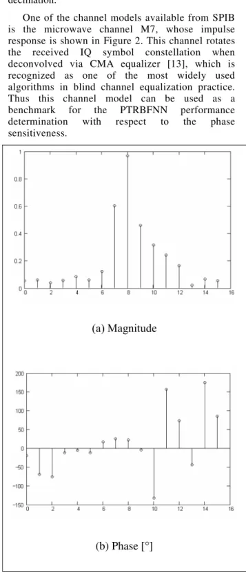
. In order to not alter the channel root locus we use frequency domain decimation.

One of the channel models available from SPIB is the microwave channel M7, whose impulse response is shown in Figure 2. This channel rotates the received IQ symbol constellation when deconvolved via CMA equalizer [13], which is recognized as one of the most widely used algorithms in blind channel equalization practice. Thus this channel model can be used as a benchmark for the PTRBFNN performance determination with respect to the phase sensitiveness.

(a) Magnitude

(b) Phase [

°

]

(7)

Besides the multipath effects represented by the channel impulse response in Figure 2, we assume an additive white Gaussian noise with Signal to Noise Ratio (SNR) of 35dB at the receiver input. The non-linear transmittance of the receiver RF front-end when operating near the upper limit of its dynamic range is also taken into account – we introduce 5% of 2nd and 3rd order harmonic distortion so that the received sequence

r

( )

n

is submitted to the non-linear relationship

( )

n r

( )

n r

( )

n r

( )

n

r_o 3

3 2

2

α

+

= ,

α

2=

α

3=0.05,

where

r

_o

( )

n

is the IQ sequence after the receiver RF front-end.

The simulation conditions are such both equalizers – the PTRBFNN equalizer and the classical complex valued RBFNN equalizer – operate in the blind concurrent architecture dictated by (23). Both equalizers share the same architectural and training parameters: L=16, K=5, 3

10 1× − = V

η

,

η

_W

=

0 .

9

,

5 .

0 =

Ψ

η

,

η

_σ

=

5 .

0

. Both equalizers also share a

common initialization procedure:

( )

[

]

T

j

V0 =0 0 0 0 0 0 0 0 1+ 0 0 0 0 0 0 0 0

,

W

(

0 )

=

0

and all the

L

components of the

k

th center initial vector Ψk

( )

0 are randomly drawn from

the 16-QAM alphabet

A

. 2

k

σ

is initialized with half the maximum Euclidean distance between all vectors

( )

0

k

Ψ

for the classical RBFNN. For the PTRBFNN,

{ }

2

Re

σ

_k and

Im

{ }

σ

k2 are initialized with half the

maximum Euclidean distance between all respective vectors

Re

{

Ψ

k

( )

0 }

and Im

{

Ψk

( )

0

}

, with

1 ,

,

1 ,

0 −

=

K

k

L

_.

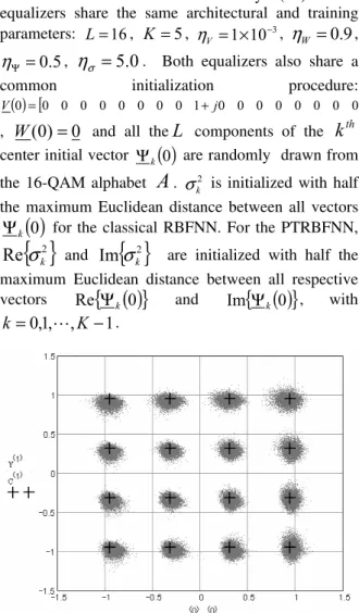
Figure 3: PTRBFNN equalizer output yafter convergence.

Figure 4: Classical complex valued RBFNN equalizer output

yafter convergence.

Figures 3 and 4 respectively show the resulting digital modulation constellations for output

y

of the PTRBFNN equalizer and for the output

y

of the classical complex valued RBFNN equalizer, after the equalizer convergence and for the previously given simulation conditions. Convergence is considered to be achieved when the output mean square error

( )

{

e

n

}

E

MSE

=

2 has decreased to a small enough value MSE

<

0 .

076

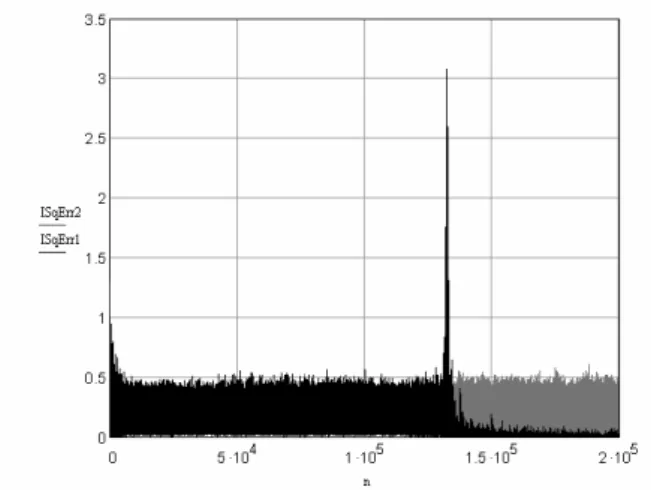
[10]. In these figures, the characters ‘+’ represent the source reference alphabet IQ symbols. Notice that the rotation of the symbols in Figure 4 with respect to the reference constellation stems from the fact that the RBFNN is not able to solve SPIB channel M7 phase distortion. Comparing Figures 3 and 4 its clear that both the RBFNN and the PTRBFNN were able to reduce the output samples dispersion, the difference being that the RBFNN output is rotated with respect to the reference constellation. This difference in terms of rotation evidences the influence of the phase transmittance on the PTRBFNN learning process, which effectively takes into account the channel phase rotation.

(8)

Figure 5: _MSE

( )

_n for the PTRBFNN equalizer (black curve) and

the classical complex valued RBFNN equalizer (gray curve).

5. C

ONCLUSION

The proposed complex valued radial basis function (RBF) neural network with phase transmittance (PTRBFNN) outperforms the classical complex valued RBF neural network (RBFNN) for those channels which impose drastic phase rotation to the received symbol sequence. The PTRBFNN not only presents a higher convergence rate than the RBFNN but also exhibits a lower steady state MSE, thus minimizing the phase invariance problem inherent to the RBFNN hidden-layer when applied to blind channel equalization. This is an important PTRBFNN feature, since adaptive joint equalization and carrier phase recovery is desirable for wireless mobile operation.

Although we have applied the new PTRBFNN to solve a specific blind channel equalization problem, its usefulness extends to any situation for which the forward transmittance of the hidden layer neurons must include phase information, such as is the case for spectral analysis in signal processing or near-field analysis in electromagnetics.

R

EFERENCES

[1] S. Chen, S. McLaughlin and B. Mulgrew: Complex-Valued Radial Basis Function Network, Part I: Network Architecture and Learning Algorithms. Signal Processing. vol. 35, pages 19-31,1994.

[2] S. Chen, S. McLaughlin and B. Mulgrew: Complex-Valued Radial Basis Function Network, Part II: Application to Digital Communications Channel Equalisation. Signal Processing. vol. 36, pages 175-188, 1994.

[3] Cha I. and Kassam S.: Channel Equalization Using Adaptative Complex Radial Basis

Function Networks. IEEE Journal on Selected Areas in Communications. vol.13, no. 1, pages.122-131, 1995.

[4] Gan Q., Saratchandran P., Sundararajan N., and Subramanian K. R.: A Complex Valued Radial Basis Function Network for Equalization of Fast Time Varying Channels. IEEE Transactions on Neural Networks. vol. 10, no. 4, 1999.

[5] Jianping D., Sundararajan N., and Saratchandran P.: Communication Channel Equalization Using Complex-Valued Minimal Radial Basis Function Neural Networks. IEEE Transactions on Neural Networks, vol. 13, no. 3, 2002.

[6] J. G. Proakis. Digital Communications, 3rd ed., McGraw-Hill, 1995.

[7] S. Haykin. Adaptative Filter Theory. 3rd

ed., Prentice Hall, Upper Saddle River, New Jersey, 1996.

[8] S. Haykin. Neural Networks. 2nd

ed., Prentice Hall, Upper Saddle River, New Jersey, 1999.

[9] S. Haykin. Blind Deconvolution. Prentice-Hall, 1994.

[10] Fernando C.C. De Castro, M. Cristina F. De Castro, Dalton S. Arantes. Concurrent Blind Deconvolution for Channel Equalization. IEEE International Conference On Communications ICC2001. page. 366-371, Helsinki, Finland , June 2001.

[11] Gitling R.D. and Weinstein S.B.: Fractionally-Spaced Equalization: An Improved Digital Transversal Equalizer. Bell Systems Technical Journal, vol. 60, 1981.

[12] SPIB – Signal Processing Information Base. http://spib.rice.edu/spib/microwave.html, http://spib.rice.edu/spib/cable.html

[13] Godard D.N.: Self-Recovering Equalization and Carrier Tracking in Two-Dimensional Data Communication Systems. IEEE Transactions on Communications. vol. COM-28, no.11, November 1980.