Climate change, farm size and land use in Brazilian Legal Amazon

MARCELO DIAS PAES FERREIRA

CLIMATE CHANGE, FARM SIZE AND LAND USE IN BRAZILIAN LEGAL AMAZON

Tese apresentada à Universidade Federal de Viçosa como parte das exigências do Programa de Pós-Graduação em Economia Aplicada para obtenção do título de Doctor Scientiae.

VIÇOSA

Ficha catalográfica preparada pela Biblioteca Central da Universidade

Federal de Viçosa - Câmpus Viçosa

T

Ferreira, Marcelo Dias Paes,

1986-F383c

2015

Climate change, farm size and land use in brazilian legal

Amazon / Marcelo Dias Paes Ferreira. – Viçosa, MG, 2015.

xi, 92f. : il. ; 29 cm.

Inclui apêndice.

Orientador: José Gustavo Feres.

Tese (doutorado) - Universidade Federal de Viçosa.

Referências bibliográficas: f.72-83.

1. Solo - uso - Amazonas. 2. Propriedade rural.

3. Mudanças climáticas - Amazonas. I. Universidade Federal de

Viçosa. Departamento de Economia Rural. Programa de

Pós-graduação em Economia Aplicada. II. Título.

MARCELO DIAS PAES FERREIRA

CLIMATE CHANGE, FARM SIZE AND LAND USE IN BRAZILIAN LEGAL AMAZON

Tese apresentada à Universidade Federal de Viçosa como parte das exigências do Programa de Pós-Graduação em Economia Aplicada para obtenção do título de Doctor Scientiae.

APROVADA: 17 julho de 2011

________________________________ Arthur Amorim Bragança

________________________________ Romero Cavalcanti Barreto da Rocha

________________________________ João Eustáquio de Lima

________________________________ Erly Cardoso Teixeira

________________________________ José Gustavo Féres

ii

ACKNOWLEDGEMENTS

First, I thank God for providing me health and serenity. I want to thank Regiane Colatini Gomes Ferreira, my wife, for her support and love during this journey. I am also grateful to my parents, Ione Maria Dias Paes and José Hélcio Ferreria (in mnmoriam), and parents-in-law, Maria Alice Soares Gomes and José Renato Gomes, for supporting me during my studies and research. Finally, I want to thank all my relatives, specially my brother, sister and brother-in-law.

iii

BIOGRAPHY

MARCELO DIAS PAES FERREIRA, son of Ione Maria Dias Paes and José Hélcio Ferreira, was born in Ervália, Minas Gerais, Brazil, in April 15th_{, 1986.}

He started his undergraduate studies at Univnrsidadn Fndnral dn Viçosa in March of 2004, receiving his B.A. in Agribusiness Management in July of 2009.

He started the M.Sc. in Applied Economics in August of 2009 and defended his dissertation titled “Impactos dos Prnços das Commoditins n das Políticas Govnrnamnntais sobrn o Dnsmatamnnto na Amazônia Lngal” in November 7th_{, 2011.}

iv

SUMMARY

LIST OF TABLES ... vi

LIST OF FIGURES ... viii

ABSTRACT ... ix

RESUMO ... x

1. Introduction ... 1

1.1. Problem and Importance ... 2

1.3. Objectives ... 6

1.3.1. General Objective ... 6

1.3.2. Specific Objectives ... 6

2. Climate Change, Climate Risk and Land Use in Brazilian Legal Amazon ... 8

2.1. Introduction ... 8

2.2. Land Use Model ... 13

2.2.1. Uncertainty ... 13

2.2.2. Land as a Fixed but Allocable Factor ... 16

2.3. Estimation and Data ... 20

2.3.1. Data ... 23

2.4. Results ... 29

2.5. Conclusion ... 42

3. Farm Size and Land Use Efficiency in Brazilian Amazon ... 44

3.1. Introduction ... 44

3.2. The Relationship between Farm Size and Productivity ... 48

3.3. Empirical Strategy ... 49

3.3.1. TE and LUE Estimation ... 53

3.3.2. Explaining LUE and TE ... 56

3.3.3. Variables and Data ... 58

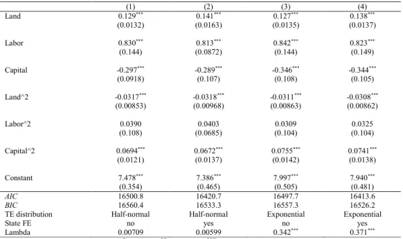
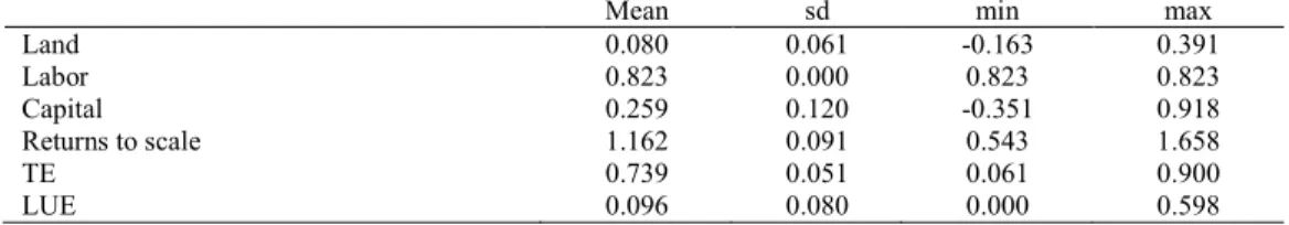
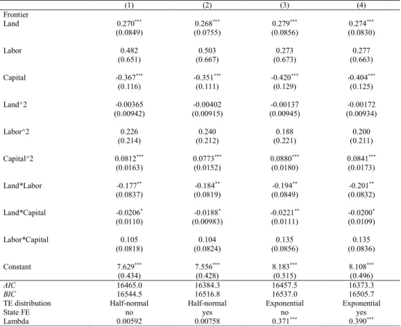
3.4. Results ... 61

v

4. General Conclusions ... 70

REFERENCES ... 72

vi

LIST OF TABLES

Table 1. Descriptive statistics of variables of interest in BLAa _{... 27} Table 2. Descriptive statistics for control variables and first-step variables... 29 Table 3. Land use equations parameters estimations for 1986-2005 climate variables for BLA in 2006 ... 31 Table 4. Land use equations parameters estimations for 1986-2005 climate variables without municipalities with irrigation or without representative farms with few respondents for BLA in 2006 ... 33 Table 5. Baseline parameters estimate (risk-averse) for land use and its risk-neutral counterpart for BLA in 2006. ... 36 Table 6. Projected land uses and percentage effects of climate change on the average BLA representative farm related to 2006 ... 40 Table 7. Percentage effects of climate change on the average state representative farms ... 41 Table 8. Descriptive statistics of variables of interest in BLA ... 61 Table 9. Estimation of technical efficiency with special case of translog production function for BLA in 2006 ... 62 Table 10. Elasticities of production, returns to scale, technical and land use

vii Table A1. Number and area of establishments by size in Brazil and BLA (1985, 1995 and 2006) ... 85 Table A2. Land use equations parameters estimations for 1946-2005 climate

variables for BLA in 2006 ... 86 Table A3. Land use equations parameters estimations for 1966-2005 climate

variables for BLA in 2006 ... 87 Table A4. Land use selection parameters estimations for 1946-2005 climate variables for BLA in 2006 ... 88 Table A5. Land use selection parameters estimations for 1966-2005 climate variables for BLA in 2006 ... 89 Table A6. Land use selection parameters estimations for 1986-2005 climate variables for BLA in 2006 ... 90 Table A7. Selection estimations for 1986-2005 climate variables without irrigated municipalities or representative farms with few respondents ... 91 Table A8. Estimation of technical efficiency with full translog production function for BLA in 2006 ... 92 Table A9. Elasticities of production, returns to scale, technical and land use

viii

LIST OF FIGURES

ix

ABSTRACT

FERREIRA, Marcelo Dias Paes Ferreira, D.Sc., Universidade Federal de Viçosa, July, 2015. Climate change, farm size and land use in Brazilian Legal Amazon. Adviser: José Gustavo Féres.

x

RESUMO

FERREIRA, Marcelo Dias Paes Ferreira, D.Sc., Universidade Federal de Viçosa, julho de 2015. Mudanças climáticas, tamanho das propriedades e uso da terra na

Amazônia Legal brasileira. Orientador: José Gustavo Féres.

1

1. Introduction

Land use is an important environmental and social attribute. Nowadays, there is a great concern regarding Greenhouse Gases (GHG) emissions and biodiversity losses due conversion of natural vegetation into agricultural land. The process of land concentration has also drawn the attention of policymakers around the world, urging a call for a more equitable agrarian organization. In this sense, Brazilian Legal Amazon (BLA) is strategic to Brazilian environmental and social achievements, since the region historically has been regarded as the main world agriculture frontier (Hecht 1985, 1993)1_{. Although deforestation in BLA has decreased during the last decade}2_, this region has presented high deforestation rates over the time. The average deforestation rate was 15,000 km2 _{over the last two decades (INPE 2015). Therefore,} deforestation and land use patterns in BLA still remains a challenging issue for policymakers.

Although the role of deforestation in GHG emissions has been extensively studied, there is a lack of literature regarding the impact of climate change on land use in BLA. Agricultural production is a source of land use change and the change on climate pattern could force farmers to adapt. For instance, areas with higher precipitation are not suitable to cattle production due to incidence of parasites and insects (Chomitz and Thomas 2003; Sombroek 2001). Furthermore, the higher the

1 _{BLA is a socio-economic region within Brazil created in 1950s for political purposes. It spans for nine}

states, covers 61% of Brazilian territory and is slight smaller than Europe. The 4 million km2 _{of Brazilian}

Amazon lies within the 5.2 million km2 _{of BLA, the remaining is mostly cerrado biome (Homma 2008;}

SUDAM 2010).

2 _{Command and control policies, monitoring systems, and supply chain interventions have reduced}

deforestation to less than 7,000 km2 _{per year since 2010 (E. Y. Arima et al. 2014; J. Assunção, Gandour,}

2 precipitation, more difficult it becomes to adopt mechanizing agriculture and slash and burn practices (E. Y. Arima et al. 2011). Thus, a lesser rainfall incidence could benefit cattle production, fostering conversion of forest into pastures.

Land concentration in BLA could also present environmental impacts in the future, as land is historically poorly distributed in Brazil and BLA (see Table A1 in appendix). About 60% of farmland belongs to establishments with more than 1,000 hectares in 2006 and these large farms represent 2.4% of the number of farms. In turn, establishments smaller than 10 hectares cover 1.33% of total farmland and corresponded to 35.4% of the number of farms. Land also has concentrated over the time in BLA. Establishments smaller than 10 hectares were 55.6% of the total and covered 1.97% of BLA farmland in mid-1980s (IBGE 2014).

This land concentration trend could be associated to a less efficient use of deforested land. In his seminal paper for Indian agriculture, Sen (1962) pointed out that agricultural productivity presents an inverse relationship with farm size. After these early findings, several studies verified this stylized fact for developing world (e.g. J. J. Assunção and Braido 2007; Bardhan 1973; Barrett, Bellemare, and Hou 2010; Bhalla and Roy 1988; Carter 1984; Cornia 1985; Newell, Pandya, and Symons 1997). If this inverse relationship holds to BLA, the land concentration process could lead to a worse utilization of deforested land. However, some studies for Brazilian agriculture have ruled out the inverse relationship hypothesis between farm size and productivity (Freitas 2014; Helfand and Levine 2004; Oliveira 2013).

1.1.Problem and Importance

3 need to assess the evolution of land use in the light of climate change and land concentration. In this study, we will focus on the relation between climate change and land use pattern as well as the issue of farm size and land productivity.

Understanding how land use patterns could respond to climate change is of paramount importance for policy formulation to BLA, as these changes could present environmental, economic and institutional consequences. For instance, annual crops stock 2.7 times more carbon than pasture in western BLA (Fujisaka et al. 1998). Secondary forest recover faster in abandoned cropland than in abandoned pasture (Fearnside 1996; Fearnside and Guimarães 1996). Pasture for cattle requires more land, demands less workforce and is less economically productive (Andersen, Granger, and Reis 1997). Forest conversion into pasture in BLA is a strategy to ensure property rights and foster land speculation (Fearnside 2001; Pacheco 2009). Furthermore, there is a need for policies of land ordering to prevent the impacts of climate change related to deforestation.

Despite the importance of comprehensive assessments of land use pattern, most of the literature have focused on the sources of deforestation in BLA3_{. Few studies} have investigated how deforested land could be allocated in competitive uses

3 _{These studies could be divided in: general analysis (Andersen 1996; A. S. P. Pfaff 1999); rural}

development and institutional perspectives (Araujo et al. 2009; Caldas et al. 2003; Marchand 2012; Perz

and Walker 2002; Sant’Anna and Young 2010; Walker, Moran, and Anselin 2000); price and

market-oriented analysis (Andrade de Sá, Palmer, and di Falco 2013; E. Y. Arima et al. 2007; Mann et al. 2010;

Mertens et al. 2002; Verburg et al. 2014); the role of the transport infrastructure (Barber et al. 2014; A.

Pfaff et al. 2007; Weinhold and Reis 2008); assessment of command and control policies (J. Assunção,

Gandour, and Rocha 2015; E. Y. Arima et al. 2014; Ferreira and Coelho 2015; Hargrave and Kis-Katos

2013; Nepstad et al. 2014); the impact of climate variables (Chomitz and Thomas 2003; Sombroek

4 (Andersen, Granger, and Reis 1997; E. Y. Arima et al. 2011; Mendonça, Loureiro, and Sachsida 2012; Weinhold 1999), and they do not analyze the mechanisms underlying land use conversion. Thus, the above-mentioned approaches do not provide an adequate framework for analyzing farmers’ adaptive strategies.

We propose an approach that differs from the current literature for BLA. First, we assess the impact of climate change by specifying a land use structural model4_, which allow us to expose the mechanisms of farmers’ adaptation to climate change. Second, we also model risk-aversion related to exogenous climate variability. This is a novelty in land use modeling and has relevant environmental policies implications. For instance, Knoke et al. (2011) found that the cost of avoided emissions from deforestation are greatly different when agents are neutral or risk-averse. In our case, accounting for risk-aversion would present an important policy insight. We argue that the fact that cattle (a low yield activity) is the dominant land use in BLA is related to agents’ risk-averse behavior. Therefore, farmers would be willing to engage in a less expected profitable activity, like cattle, if it is also less risky.

The inverse relationship between farm size and agricultural productivity also presents environmental policy implications. The main explanations for this relationship relies on labor effectiveness differences associated to dual labor market (Sen 1962; Sen 1966), risk-aversion (Barrett 1996; Srinivasan 1972), and moral hazard

4 _{Our land use structural model is based on studies for other contexts (Arnade and Kelch 2007;}

Chambers and Just 1989; Coyle 1993a; Coyle 1993b; Fezzi and Bateman 2011; Fezzi et al. 2014;

Gorddard 2013; Heres, Ortiz, and Markandya 2013; Kaminski, Kan, and Fleischer 2012; Lacroix and

5 and supervision of labor (Bardhan 1973; Eswaran and Kotwal 1986; Feder 1985)5_. These three explanations predict that farm size is negatively associated to productivity. One could measure agricultural productivity by some efficiency indicator, representing total factor productivity (Helfand and Levine 2004). In this sense, technical inefficiency is a measure of resource waste related to the best-observed practice. Thus, more efficient farms would spare land, reducing the need for deforestation. In the BLA context, Otsuki, Hardie, and Reis (2002) found that well-defined property rights enhance economic efficiency, reducing the need for more deforestation. Helfand and Levine (2004) identified a “U” shaped relationship between farm size and technical efficiency in Brazilian mid-west. Thus, both larger and smaller farms are more efficient than median farms. Finally, Marchand (2012) assess the relationship between technical efficiency and deforestation in BLA. He found a “U” shaped relationship, where less and more efficient farms deforest more than average efficient farms.

Nonetheless, all of the above-mentioned studies have used a misleading measure to gauge the surplus of land used in agricultural production. The recurrent technical efficiency approach capture the misuse of all inputs and do not provide a single measure of land waste. The surplus of land is associated to the amount of avoided deforestation without compromise the actual agricultural production. Therefore, there is a need of a land efficiency indicator based on an input-specific technical efficiency to gauge land surplus. Reinhard, Lovell, and Thijssen (1999) provide an approach to measure input waste associated to an environmental attribute. This approach consists in analyze the ratio of the minimum possible use of a single

5 _{See section 3.2. “The Relationship between Farm Size and Productivity” for further details on}

6 input between the best observable use of this factor, keeping constant the level of output and other inputs. We used this latter approach in order to measure land waste in BLA.

1.2.Hypotheses

 Pasture establishments are a hedge strategy to climate risk in Brazilian Legal Amazon;

 Climate change will increase land allocation in pastures and decrease land allocation in crops and forest in Brazilian Legal Amazon;

 There is an inverse relationship between farm size and productivity across Brazilian Legal Amazon.

1.3.Objectives

1.3.1. Gnnnral Objnctivn

 Assess land use pattern in Brazilian Legal Amazon, highlighting the role of climate change and farm size.

1.3.2. Spncific Objnctivns

 Clarify farmers’ decision of land use allocation;

 Identify the impacts of climate change on land use;

 Analyze the relationship between farm size with technical efficiency and land use efficiency.

8

2. Climate Change, Climate Risk and Land Use in Brazilian Legal Amazon

2.1.Introduction

Global climate change will likely have adverse consequences on agriculture. In the near future, rural areas will probably face impacts on water availability and supply, food security, and agricultural incomes (IPCC 2014). Climate change will also modify climate variability pattern. For instance, more extremes events are likely to occur such as droughts and heat waves (IPCC 2014).

Brazil provides a compelling setting for studying the effects of climate change on agriculture. First, Brazil is currently the fourth worldwide producer and exporter of agricultural goods (FAO 2015). Second, the country has experienced a boom in agricultural sector since 1970s. Agricultural expansion has triggered the conversion of vegetation into agricultural use, especially in Amazon and cerrado biomes. In fact, Brazilian Legal Amazon (BLA)6 _{is regarded as the main agricultural frontier} worldwide. Although deforestation in BLA has decreased during the last decade, it still presents high values. For instance, average deforestation rate has been 15,000 km2 per year over the last two decades (INPE 2015). Recently, command and control policies, monitoring systems, and supply chain interventions have reduced deforestation to less than 7,000 km2 per year since 2010 (J. Assunção, Gandour, and Rocha 2015; Hargrave and Kis-Katos 2013; Ferreira and Coelho 2015; Nepstad et al. 2014; Richards, Walker, and Arima 2014). Third, Brazil was the sixth GHG emitter

6 _{BLA is a socio-economic region within Brazil created in 1950s for political purposes. It spans for nine}

states, covers 61% of Brazilian territory and is slight smaller than Europe. The 4 million km2 _{of Brazilian}

Amazon lies within the 5.2 million km2 _{of Brazilian Legal Amazon. The remaining is mostly cerrado}

9 country in 2011, accounting for 3.1% of world emissions (WRI 2015). Agricultural and land use change is identified as the main source of GHG emissions in Brazil7_{. BLA} has substantially contributed to Agriculture, Forestry and other Land Use (AFOLU) emissions, since it represents Brazil’s main agricultural frontier. Therefore, what happens in BLA regarding land use is of global concern.

Several studies have analyzed the role of land use change in BLA on GHG emission mitigation (e.g. Cohn et al. 2014; Santilli et al. 2005; Stickler et al. 2009; Strassburg et al. 2009). However, few studies have been devoted to assess the inverse relation, the effect of climate change on land use patterns in BLA. Climate change is likely to influence land use patterns in BLA, since farmers would adapt to this phenomenon. Changes in temperature and rainfall variability could also lead to changes on land use decisions due farmers’ risk-aversion. Climate change can induce more forest conversion into agricultural land. This would increase GHG emission related to agriculture. Climate change may also induce conversion of cropland into pasture. All these changes present important environmental and economic consequences. Therefore, there is a need to assess these potential impacts.

There are three main approaches to measure impacts of climate change on agriculture: Agronomic/Production Function; Ricardian/Hedonic; and Computable General Equilibrium (CGE) models8 _{(Fezzi et al. 2014; Schlenker, Hanemann, and}

7 _{Agriculture, forestry and other land use (AFOLU) accounted for 24% of worldwide GHG emissions}

in 2010 (IPCC 2014). AFOLU GHG emissions in Brazil accounted for 57% for the same year (BRASIL

2013).

8 _{See Adams (1989) and Adams et al. (1995) as examples of Agronomic/Production Function approach;}

Mendelsohn, Nordhaus, and Shaw (1994), Schlenker, Hanemann, and Fisher (2005, 2006), and

Deschênes and Greenstone (2007) as examples of Ricardian/Hedonic approach; and Hertel, Burke, and

10 Fisher 2006). The Agronomic approach evaluates the direct impact of climate change on yields. However, this approach implicitly relies on the so-called “dumb farmer” hypothesis, since it does not consider a broad range of adaptive strategies. Failing to address adaptation strategies tends to overestimate the impact of climate change (Fezzi et al. 2014; Mendelsohn, Nordhaus, and Shaw 1994). The Ricardian/Hedonic approach, on its turn, consists in the estimation of a reduced form equation of farmland values/land rents that includes a set of climate variables as regressors. While this approach accounts for adaptation, it does not provide information about farmers’ adaptive strategies (Fezzi et al. 2014). Finally, CGE models endogenize prices and account for inter-sectorial and international linkages (Fezzi et al. 2014; Schlenker, Hanemann, and Fisher 2006). However, these advantages come at the cost of aggregated analysis of entire economic sectors. This implies a loss of information regarding heterogeneity and spatial variation in environmental variables (Fezzi et al. 2014).

11 Although the impact of changes in mean temperature and rainfall on agriculture has generated a great deal of interest, the role of variance changes of these climatic variables has not gained similar attention. A larger climatic variance increases the variance of farm profits, which might induce risk-averse farmers to change their decisions. Notwithstanding, few studies have analyzed adaptation strategies to changes in climate variability. A Ricardian study found that climate variability have affected land prices in mid-western U.S. (Kelly, Kolstad, and Mitchell 2005), whilst other found a negative relationship between land prices and rainfall variability in Brazil (Cunha, Coelho, and Féres 2015). Kaminski, Kan, and Fleischer (2012) used a structural model to evaluate the impact of rainfall variability on Israeli agriculture. They found that higher inter-annual rainfall standard deviation is associated to more surface allocated to irrigated crops. However, Kaminski, Kan, and Fleischer (2012) set up a risk-neutral theoretical model. This could prevent correct estimation of parameters, once the certainty results regarding agents behavior are biased if agents are risk-averse (Pope 1982). Coyle (1999) proposed a more suitable approach to incorporate climate variability by considering a risk-averse utility maximization framework. This approach avoids biased estimates by imposing theoretical restrictions on the specifications of the land use model.

12 authors stated that this pattern occurs because cattle production in BLA is more profitable than in other Brazilian regions due to a higher productivity and a lower land cost (E. Arima, Barreto, and Brito 2005; Walker et al. 2009). Nevertheless, the latter did not dismiss the profitability gap between cattle production and other agricultural activities. We propose an alternative explanation based on portfolio theory. Pasture for cattle production could be a hedging strategy for risk-averse farmers if other land uses present a higher yield variability related to climate variability. Therefore, farmers would be willing to engage in a less profitable activity, like cattle, if it is also less risky. This behavior presents important policy implications9_{. For instance, there will be more} land allocated into pasture in the near future if climate change leads to a higher climate variability.

To properly account for climate variability, we bring together two important strands of the literature in our theoretical model. First, following Chambers and Just (1989), we consider land as a fixed but allocable factor to deal with two aspects of agricultural production: spatially separated production and cross-output interdependence. This is the most frequent approach adopted by risk-neutral land use studies (e.g. Arnade and Kelch 2007; Fezzi and Bateman 2011; Fezzi et al. 2014; Kaminski, Kan, and Fleischer 2012; Lacroix and Thomas 2011). Second, we add risk-aversion related to exogenous climate variables to Chambers and Just (1989) approach. This is a novelty in land use modeling, since risk-averse land use models do not rely on Chambers and Just (1989) approach and do not model climate variability as a source of yield risk (e.g. J.-P. Chavas and Holt 1990; J. Chavas and Holt 1996; Komarek and Macaulay 2013; Lansink 1999).

13 The remainder of this chapter is organized in the following way. After this introduction, section 2.2 presents the land use risk-averse model. Section 2.3 discusses the estimation procedure and describes the database. Section 2.4 presents results and the simulation exercises regarding the impact of climate change on land use patterns. Finally, section 2.5 consolidates the main conclusions and points out potential policy implications.

2.2.Land Use Model

Our theoretical model consists of a two-step maximization problem where technology is nonjoint among land uses. However, crops compete for a fixed amount of land, implying land use interdependence10_{. At first-step, farmers maximize utility} from each land use given the allocation of land and other fixed inputs. In this step, we show the utility maximization problem under uncertainty in a Coyle's (1999) approach. In the second-step, we treat land and other fixed inputs as fixed but allocable factors, a framework proposed by Chambers and Just (1989).

2.2.1. Uncnrtainty

Climate uncertainty modeling relies on the assumption that farmers know the probability distribution of climate variables. This is a proxy for farmers' climate perception rather than real farmers’ rationalization. They do not know these variables exactly, but they should know which locations have a high level of expected precipitation or high climate variability. We assume that farmers are characterized by a constant absolute risk aversion (CARA) behavior; technology may be described

10 _{Chambers and Just (1989) argues that multioutput agricultural production can be described by}

14 according to Just and Pope (1978, 1979) and there is no price uncertainty in our framework. Our approach, rather restrictive, is recurrent in production analysis as it simplifies duality results and empirical applications (Coyle 1999)11_.

The utility function (U) of risk-averse farmer can be represented by his

certainty equivalent, which is linear in expected profits ( ) and profit variance (_2₎

2

) 2 ( 

 r

U  (1)

where r is the coefficient of risk-aversion.

Profits from a land use “i” are

wx y p_{i i}

i 

 ₍₂₎

where pi is output price related to a land use; yi is the output quantity related to land

use “i”;

w

is the price vector of variables inputs; and

x

is the vector of variable inputs.

According to Coyle (1999), the Just and Pope (1978, 1979) production function could take the following form for each land use

) , ( ) , , ( ) , ,

(x z l b x z l 12d c₁c₂ a

y_i _{i i i i}  _{i i i i i} (3)

11 _{These assumptions are not necessarily realistic for BLA. We did not rely on stronger assumptions}

like Decreasing Absolute Risk Aversion (DARA) utility function due lack of data on farmers’ wealth.

15 where

z

i is a fixed input, like capital, allocated to production of yi; li is the land

allocated to production of yi; and di(c1,c2) is a underlying climate attribute variable

which is a function of temperature  c1 and rainfall  c2 .

The first term in the right-hand side of (3) is nonstochastic, since farmer chooses the quantity of variable and fixed inputs to be used in the production of yi, as

well as the surface allocated to this land use. The second term in the right-hand side of (3) is stochastic. Climate attribute is a nonlinear function of stochastic climate

variables12 _and b_i(x_i,z_i,l_i)12 _{is a term added to account for inputs that increase}

production variability and inputs that decrease production variability13_.

Using equations (2) and (3), one can show that expected profits (i ) and

profits variance (2i) are

wx c c d l z x b p l z x a

p_{i i i i i i i i i i i}

i ( , , ) ( , , )12 (1, 2)

 (4)

) , , ( ) , ,

( ₁₂

2 1 2 2 2 2 2 2 2 c c c c di i i i i i yi i

i p pb x z l    

_   ₍₅₎

Replacing (4) and (5) in (1) and solving for xi yields

12 _{This assumption differs from Coyle (1999), where}

i

y is an increasing function of climate variables.

We assume that yi is an increasing function of id(c,1c2), a nonlinear function of climate variables.

13 _{Just and Pope (1979) pointed out that agriculture output variance is an increasing function of inputs}

in traditional specifications of production functions. This is not a reasonable result for inputs like

pesticides and irrigation equipment, since output variability appears to be a decreasing function in these

16 )} , , ( ) , , ( ) 2 ( ) , ( ) , , ( ) , , ( { max } ) 2 ( { max ) , , , , , , , , ( 2 1 2 1 2 1 2 1 2 2 2 2 2 1 2 1 0 2 2 0 2 2 2 1 c c c c di i i i i i i i i i i i i i i i i i x yi i i i i x c c c c i i i i l z x b p r wx c c d l z x b p l z x a p p r wx y p c c l z w p v                  (6)

Assuming that indirect utility function v_i() exists and is twice differentiable,

Coyle (1999, pp.554–555) generalized the duality results under output uncertainty:

) (

i

v is linear homogenous in (pi,w1,/c2₁1,/c2₂1,/c₁c₂)14; expected output supply,

variable inputs demands and output variance can be recovered by generalizations of

Hotelling’s lemma (y_iv_i() p_irp_i_yi2 _,xv_i()w_,2_yiv_i() _di2(2_di2)/(rp_i2)_{); and}

) (

i

v is convex in input prices

w

but not in (pi,w).

2.2.2. Land as a Fixnd but Allocabln Factor

We assume that farmers could produce three aggregate outputs related to each land use “i”: 1=cropland, 2= pasture and 3=forest. Thus, there is an indirect utility

function

v

i

(



)

to each land use. Each farmer has an endowment of land L and other

quasi-fixed inputZ , which are allocable to different land uses. Following Chambers

and Just (1989), the farmer maximizes the constrained problem in li and zi

14 _{Linear homogeneity results rely on assumption that} 2₍ 2_, 2_{, )} 2₍ 2_, 2_{, )} 2 1 2 1 2 1 2

1k c k cc k di c c cc

c k

di       

  _.

Assuming an optimal xi in right-hand side of expression (6) and the later assumption yields

) , 2 , 2 , 2 ,1 , , , , ( ) , 2 , 2 , 2 ,1 , , , ,

( ₁₂

2 1 2

1 2

1 k c k cc k kvi ipw izilcc c c cc

c c c il iz kw i kp

17                     







   3 1 3 1 3 1 2 2 2

1, , , , )

, , , ,

( ₁₂

2 1 i i i i i c c c c i i i

i p wz l c c L l Z z

v     

L (7)

 _and  _{are the Lagrange multipliers for land and other quasi-fixed inputs,}

respectively. First order conditions for an interior solution of the Lagrangean are expressed by 0 ) ( _{ }       _ i i i l v l L ₍₈₎ 0 ) ( _{ }       _ i i i z v z L ₍₉₎ 0 3 1  



 i i l L ₍₁₀₎ 0 3 1  



 i i z Z ₍₁₁₎

18 The system (8)-(11) of 6 equations and 6 unknowns yields optimal solution to the constrained multi-output optimization problem in (7)15_:

) , , , , , , , ,

( ₁₂

2 1 2 2 2 1 * c c c c i pwZLc c

l    _and ( , , , , , , , , ₁₂)

2 1 2 2 2 1 * c c c c i pwZLc c

z    _{. Substituting} l_i*() _and

) (

*_ i

z _{in (10) and (11) yields identities of physical conservation laws (Moore and Negri}

1992). Differentiating land identity 0

3 1 *_ 



 i i l

L _in p ,

w

, Z , L , c1, c2,

2

1

c

 _, _c2_{2 ,}

and c₁c₂ yields

1 3 1 *   



 i i L l

; 3 0

1 *   



 i i Z l

; 3 0

1 *   



 i j i p

l _; 3 ₀

1 *   



 i i w l 0 3 1 *   



 i h i c l

; 3 0

1 2 *   



 i c i h l

 ; 0

3 1 * 2 1   





i cc

i

l 

(12)

where j = 1 (cropland), 2 (pasture) and 3 (forest); h = 1 (temperature) and 2 (rainfall). The first identity in (12) states that an additional unit of land should be fully allocated among uses. Other identities state that changes in other variables are fully absorbed within the land endowment L.

Coyle (1999) used normal quadratic (NQ) flexible form to parameterize v_i()

for empirical purposes16_{. Defining}

w

_{as agricultural wages and Z a fixed input, vi()}

15 _{Note that} *

i

l and z_i* is a function of all output prices ( p vector) rather than own output price (pi).

This occurs because changes in own price modify marginal utility of a land-use, which lead to changes

in other land-use allocation to equate their marginal utilities.

16 _{NQ was first proposed by Lau (1976) and is a Taylor’s expansion of second order. NQ has the}

19 linear homogeneity propriety ensures that prices, climate variability and utility could

be expressed relative to the price of numéraire input

w

:

p

i*



p

i

/

w

,  c2₁* wc2₁,

2 * 2

2 2 c

c w

  _, *_c1c2w_{12, and} v_i*()v_i(/)w_{. Assuming}

) , , , , , , , ( ) ,...

( 2* 2* *

2 1 * 1 2 1 2 1 c cc

c i

i i

M _{p z l c c}

n n

n 







_{, NQ is expressed as}

 

 



    i j j i ij i i i

i n nn

v*() ₀  12  , with  _ij _ji.

When utility functions are NQ, one can write l*i() as

* 10 * 2 9 * 2 8 2 7 1 6 5 4 3 1 * 0 * 2 1 2

1 i c i cc

c i i i i i j ji j i

i p L Z c c

l  



          

 (13)

Restrictions in (12) imply that



_4i1_and



_ji0 _{for j 4. The effect on}

land use allocation of a change in variances follows the portfolio theory. For instance,

an increase in rainfall variability ( 2

2

c

 ) will increase yield risk in all three activities

cntnris paribus. These effects are likely to vary across activities due differences in each

climate attribute function

d

i

(

c

1

,

c

2

)

. The farmer would reallocate land among uses to

equate his/her marginal land use utilities and achieve a new equilibrium. The activity which yield risk is less sensitive to the change of climate variability will absorb land

is a matrix of constants – once reached, optimal sufficient conditions hold globally; the first derivatives

are linear in prices and fixed inputs; and maintains linear price homogeneity (Shumway 1983, 749–50).

Furthermore, NQ is preferable than traditional Cobb-Douglas and Translog specification because it does

20 from other uses, as expressed by



_9i0_{. Therefore, the farmer would choose the}

less risky portfolio given the expected returns.

As Gorddard (2013, p.1114) pointed out, dual results of cross-price symmetry in output supply and input demand do not hold in (13) (i.e. assumption of  ji ij for

prices does not occur due to land allocation is a primal result). However, Gorddard (2013) demonstrated an equivalent symmetry result for land as fixed but allocable

factor: li pj_yi Ll_i L_lj pi_yj Ll_j L_, for i j. In other words, cross-price

symmetry holds when corrected by marginal effect of L on yields.

2.3.Estimation and Data

A suitable empirical strategy to estimate the system of equation (13) is seemingly unrelated regressions (SUR), once this technique accounts for cross-equational error correlation. However, it does not deal with censoring that arises from corner solutions in the farmer maximization problem. In fact, zero allocation is frequent in farm level analysis and is present in this study, censoring each land use from below. A primary choice to deal with this issue is a SUR-Tobit estimator. However, Shonkwiler and Yen (1999) pointed out that system estimation with censored dependent variables is computationally demanding, since it requires the evaluation of multiple integrals in the likelihood function.

21 and Deal 2004; Goodwin and Mishra 2005; Goodwin and Mishra 2006; Sckokai and Antón 2005; Sckokai and Moro 2006; Sckokai and Moro 2009; Platoni, Sckokai, and Moro 2012).

In our application, the first-step consists in estimating a probit model of land use decisions to retrieve the cumulative distribution function and the normal probability density function for each land use decision. This is a selection step to model binary farmer’s decision regarding to set or not to set a land use. Notwithstanding, the main Shonkwiler and Yen (1999) contribution consists in the second-step. They found that the intuitive system of equation generalization of Heckman’s sample selection procedure proposed by Heien and Wessells (1990) is not consistent, generating biased unconditional expectations of dependent variables. Furthermore, Shonkwiler and Yen (1999) stated that estimation of a censored system requires a procedure that uses the entire sample since each dependent variable could present a different pattern of censoring in terms of limit and nonlimit outcomes17_{. In order to overcome these latter} drawbacks in the second-step procedure, Shonkwiler and Yen (1999) proposed the SUR estimation of the following system for the entire sample in the second-step

ij

i

ij

z

i

i

ij

x

f

i

ij

z

ij

l























                

_'

_,

_'

_, 3 , 2 ,1  i (14)

17 _{For example, a farm with zero land allocation in crop is likely to present nonzero land allocations in}

other land uses. If this farm is dropped from the second-step estimation due zero allocation in crops, we

22 where j is farms; 

    

i

ij

x

f

,



is the land use allocations equation expressed in (13);

     



z

'

_ij



_i

and    

 

i

ij

z





'

are the cumulative distribution function and normal density

function, respectively, obtained in the first-step;



_i

is the unknown coefficient of

correction factors;

x

_ij

and

z

_ij

are vectors of exogenous variables18_;

i

 and



_i

are

vectors of first and second-step parameters, respectively; and



_ij

is the error term with

zero mean.

The Shonkwiler and Yen (1999) procedure has received criticism due its lack of estimation efficiency related to its heteroskedastic errors (Tauchmann 2005, 2010). To deal with this drawback and improve estimation efficiency, we estimated (14) and bootstrapped the residuals with 300 replications clustered by municipality, which also dealt with potential spatial autocorrelation. We estimated the first-step in a probit multivariate system by a methodology proposed by Roodman (2011), which provides enhanced estimates by considering potential correlation of errors term in probit equations (Platoni, Sckokai, and Moro 2012). Adding-up restrictions for observed land allocations leads to a singular estimation matrix. In order to overcome the singularity problem, system (14) was estimated by excluding the forest equation. Once crop and pasture equation parameters are estimated, forest coefficients can be recovered from the restrictions expressed by (12).

18 _{As in traditional sample selection models,}

ij

x is a subset of z_ij and the later are the explanatory

variables in the first-step. Platoni et al. (2012) suggests the addition of demographic variables in x_ij to

23

2.3.1. Data

We used data from Brazilian Agricultural Census of 2006 on land use pattern, a proxy to capital endowment and agricultural wages. The Brazilian Institute of Geographic and Statistics (Instituto Brasilniro dn Gnografia n Estatística – IBGE) provides this information on municipal level segmented into five land tenure groups (owner, sharecropper, renter, occupant and farmers recently granted in land reform (less than five years)) and eleven farm-size groups19_{. We created representative farms} from averages of each group formed from a municipality “i”, land tenure “j” and farm size group “k”. Thus, each municipality could present up to 55 of these representative farms. Pasture allocations are the sum of native and cultivated pastures, while forestland is obtained by adding up native and cultivated forests. Cropland is computed in a residual manner, by subtracting pasture and forest from total area20_{. We did not} use the cropland allocations present in the census to avoid double counting, as the same surface would be used to grow more than one crop within a year. For example, in some BLA regions farmers grow soybean during spring/summer and maize during autumn/winter in the same surface. Total farm area and all land allocations are expressed in hectares (10,000m²). A proxy for capital is the declared value of all vehicles in each representative farm in rnal (Brazilian currency), and represents tractors and other vehicles used in agricultural production. Wages are computed as the value of total wages paid to workers divided by a labor variable equivalent to an eight hours workday.

19 _{This is a special tabulation of Census constructed from IBGE microdata. We are grateful to Eustáquio}

Reis from IPEA for providing us this dataset.

20 _{In computing total farm area, we ignored buildings areas, areas covered with water and land unsuitable}

24 Prices of cropland and forest products are regional price indexes for the 1996-2005 calculated from data of IBGE yearly agricultural and forestry surveys (Produção Agrícola Municipal and Produção da Extração Vngnral n da Silvicutura, respectively). Crop prices index aggregates prices of 18 agriculture products that corresponds to 98.4 % of agricultural production value in Amazon in 200621_{. Forest prices aggregate six} products of natural and planted forest, covering 98.1% of forest production22_{. We} deflated the value of production to 2005 values using the General Index Price provided by Institute for Applied Economic Research (Instituto dn Pnsquisa Econômica Aplicada – IPEA) website (www.ipeadata.gov.br). The real prices for each product are the quotient between the value of production for 1996-2005 period and the amount of production for the same period. We calculated the index for each municipality using

the formula: 

_

n_

_

_{ij j}

j qijpij q p

RPI

1 . Where i are the municipalities; j are the 18 agricultural products or the 6 forest products, qij is the amount produced of j in

municipality i; pijis the average real price of product j in municipality i; pj is the

average price of product j in Legal Amazon. Pasture output prices are the municipal cattle price for 2001 computed by Arima et al. (2007). This is an average farm-gate price by municipality built from slaughterhouses beef prices discounting the transportation costs. We normalized prices indexes and wages index at the mean and multiplied by 100.

Climate variables were provided by Professor Claudio Araujo from Centre d’Études et de Recherches sur le Développment International (CERDI)/Université

21 _{Pinapple, cotton, rice, sugar cane, beans, cassava, watermelons, maize, soybean, banana, ruber, cocoa,}

coffee, coconut, palm oil, oranges, and black pepper.

25 d’Auvergne, France. This database consists in the Willmott, Matsuura and Collaborator’s (http://climate.geog.udel.edu/~climate/) data on monthly temperature (in Celsius degree) and rainfall (in millimeters) converted to Brazilian municipalities boundaries by Simonet (2013). We built the climate variables as follows. Mean temperature is the average annual mean temperature. Accumulated rainfall is the average of annual accumulated rainfall. Inter-annual temperature variance is the variance of annual average temperature. Inter-annual rainfall variance is the variance of annual accumulated rainfall. Inter-annual climate covariance is covariance of annual mean temperature and annual accumulated rainfall. Intra-annual temperature variance is the average between years of monthly temperature variance within years. Intra-annual rainfall variance is the average between years of monthly rainfall variance within years. Intra-annual climate covariance is the average between years of monthly temperature and rainfall covariance within years. The first five variables are the climates variables in expression (13). Inter-annual variances and covariance provide information about probability of a year with extremes climate events, such a drought or a higher temperature. Intra-annual variances and covariance provide information on the average seasonal pattern. Municipalities with higher average intra-annual variances indicate that seasons are more heterogeneous. Positive intra-annual covariance indicates that temperature and rainfall move in the same direction in the seasons. Negative intra-annual covariance indicates that these variables move in different directions. We built climate variables for three time spans (1946-2005, 1966-2005, and 1986-2005) to explore farmer’s different behavior with respect to time horizon of climate variables.

26 The mean price indexes and wages index differ from 100 because we dropped some missing values in other variables. Regarding censoring in land use, 2% of the sample presented zero allocation in cropland, 14% in pasture, 17% in forest. The only climate variables that substantially differ between the three periods are inter-annual rainfall variance, inter-annual climate covariance and intra-annual climate covariance. Inter-annual rainfall variance has decreased in last period compared to the two previous, as well its variability between municipalities. Absolute inter and intra-annual climate covariance increased over the period. Linear homogeneity is imposed by dividing all price indexes by wages. Similarly, we multiply inter-annual variances and inter-annual climate covariance by wages. Intra-annual variables appear in the models without transformations.

27 Table 1. Descriptive statistics of variables of interest in BLAa

mean sd cv min max

Cropland (ha) 15.90 137.72 8.66 0.00 6908.71

Pasture (ha) 107.69 626.66 5.82 0.00 16017.40

Forest (ha) 89.93 679.16 7.55 0.00 22569.51

Land (ha) 213.52 1257.12 5.89 0.00 33329.84

Capital (R$) 23349.90 386278.88 16.54 0.00 24230400.00

Observations per representative farms 229.07 420.65 1.84 3.00 6095.00

Crop price index 99.85 34.55 0.35 47.17 350.05

Cattle price index 99.95 15.57 0.16 7.64 120.58

Forest price index 99.48 38.27 0.38 29.39 347.61

Wages index 102.73 123.33 1.20 5.70 769.43

Mean temperature (Celsius)

1946-2005 25.36 1.20 0.05 17.85 28.20

1966-2005 25.47 1.19 0.05 17.95 28.40

1986-2005 25.76 1.17 0.05 18.40 28.61

Accumulated rainfall (mm)

1946-2005 1883.99 394.72 0.21 1102.71 3052.11

1966-2005 1903.72 397.63 0.21 1138.36 3066.16

1986-2005 1896.75 423.37 0.22 1078.70 3163.58

Inter-annual temperature variance (Celsius2₎

1946-2005 35.77 73.06 2.04 0.62 851.99

1966-2005 40.90 86.92 2.13 0.64 1022.47

1986-2005 32.24 71.01 2.20 0.65 802.26

Inter-annual rainfall variance (mm2₎

1946-2005 5787212.92 7498822.49 1.30 4108.24 1.99e+08

1966-2005 5614384.84 6953624.49 1.24 3794.73 1.87e+08

1986-2005 4554352.62 5365889.86 1.18 2641.23 76947880.00

Inter-annual climate covariance

1946-2005 656.44 2955.18 4.50 -10896.02 20827.44

1966-2005 187.21 2492.54 13.31 -17618.38 14694.88

1986-2005 2031.04 3314.36 1.63 -12659.48 25248.94

Intra-annual temperature variance (Celsius2₎

1946-2005 0.96 0.91 0.95 0.23 4.78

1966-2005 0.95 0.89 0.94 0.22 4.66

1986-2005 0.99 0.87 0.88 0.25 4.81

Intra-annual rainfall variance (mm2₎

1946-2005 16781.00 5164.83 0.31 6823.20 42555.24

1966-2005 16537.93 5017.32 0.30 6410.68 43196.08

1986-2005 16327.86 5130.14 0.31 7052.56 42435.86

Intra-annual climate covariance

1946-2005 -3.50 57.88 -16.56 -126.41 225.80

1966-2005 -3.18 57.60 -18.13 -124.93 226.66

1986-2005 -12.68 59.16 -4.66 -125.70 207.22

a. Cropland, pasture, forest, land, and capital vary between and within municipalities. Other variables

vary only between municipalities. sd – standard deviations; cv – coefficient of variation; min –

minimum; max – maximum.

28 1 and the reference for topography is topography class 2. We did not use topography 1 in estimations because it is rare class within Amazon, which could lead to multicolinearity. To account for biome differences, we introduced the percentage of municipalities areas covered with cerrado biome. We expect that the forest output bundle in cerrado differ from Amazon, the dominant biome within BLA. For example, vegetation in cerrado is sparser than in Amazon biome. Thus, it is less productive in wood products. This could affect the forest profits as well as land use allocation. Soil, topography, and biome data are provided by the Center for Studies and Spatial Systemic Models (Núclno dn Estudos n Modnlos Espaciais Sistêmicos - NEMESIS). Latitude controls, among other factors, for the incidence of solar radiation. This variable is the absolute latitude of municipalities centroids provided by IBGE. The third set of variables relates to institutional environment indicators provided by Catholic Pastoral Land Commission for 2005. These variables are the number of rural conflicts per municipality, the number of murders and murders attempts related to land per municipality, and the number of farms caught with slavery and poor work conditions per municipality. Araujo et al. (2009) showed that these institutional variables are associated to property rights in BLA and weak property rights increases deforestation.

29 Table 2. Descriptive statistics for control variables and first-step variables

mean sd cv min max

Owner (proportion) 0.6775 0.4675 0.69 0.00 1.0

Settled (proportion) 0.1114 0.3147 2.82 0.00 1.0

Renter (proportion) 0.0525 0.2230 4.25 0.00 1.0

Sharecropper (proportion) 0.0523 0.2227 4.26 0.00 1.0

Ocupant (proportion) 0.1062 0.3081 2.90 0.00 1.0

% soil type 1 4.2727 16.2268 3.80 0.00 100.0

% soil type 2 3.6750 16.2344 4.42 0.00 100.0

% soil type 3 3.0463 12.7680 4.19 0.00 100.0

% soil type 4 44.7235 38.6824 0.86 0.00 100.0

% soil type 5 2.5322 12.9147 5.10 0.00 99.4

% soil type 6 4.6935 16.9302 3.61 0.00 100.0

% soil type 7 0.3677 3.8447 10.46 0.00 72.0

% soil type 8 36.6785 38.8318 1.06 0.00 100.0

% topography type 2 36.6785 38.8318 1.06 0.00 100.0

% topography type 3 4.2275 16.5783 3.92 0.00 100.0

% topography type 4 56.1215 38.6304 0.69 0.00 100.0

% topography type 5 2.4959 12.9113 5.17 0.00 99.4

Latitude (dgrees) 7.2154 4.3461 0.60 0.03 16.8

%Cerrado 31.5411 44.3547 1.41 0.00 100.0

Conflict (occurrence) 0.6609 1.5248 2.31 0.00 15.0

Slavery/Poor work conditions (occurrence) 0.4967 1.8583 3.74 0.00 20.0

Murder/Attempts (occurrence) 0.0664 0.4206 6.33 0.00 5.0

Education (proportion) 0.3083 0.1184 0.38 0.00 1.0

Experience (proportion) 0.1869 0.1092 0.58 0.00 1.0

Women (proportion) 0.0344 0.0413 1.20 0.00 0.7

Younger than 25 (proportion) 0.0166 0.0298 1.80 0.00 0.6

Older than 55 (proportion) 0.1259 0.0810 0.64 0.00 1.0

sd – standard deviations; cv – coefficient of variation; min – minimum; max – maximum.

2.4.Results

Results for the climate variables for three different time spans (1946-2005, 1966-2005, and 1986-2005) are in Table A2, Table A3 and Table 3 respectively23_. There are three specifications in each of the three tables. Column 1 presents results using only land tenure as control variables. Column 2 presents results controlling for land tenure and agronomic variables. Column 3 introduces institutional variables as additional controls. We presented results in this way to verify parameters stability related to control variables. We suppressed control variables parameters to save space. Thus, we do not report results for land tenure dummies, soil quality, topography

23 _{Table A2 and Table A3 are presented in the appendix, since the results for the 1986-2005 in Table 3}

presented a better fit. First-step estimations considering the different climate variables time span are

also in appendix: Table A4, Table A5 and Table A6, respectively. In the first-step tables, we do not

30 quality, latitude, cerrado share, conflicts, slavery/poor work conditions, and murder/attempts.

Results for the 1946-2005 time span do not show a strong relationship between land use allocation and climate variables. The significant climate variables in each specification are accumulated rainfall and intra-annual temperature variance in the pasture equation. Accumulated rainfall coefficients for cropland become significant in the column 2 and 3. Accumulated rainfall and intra-annual coefficients in pasture equation present an absolute increase when we introduce agronomic variables. Inter-annual temperature variance coefficient for cropland equation is significant at 10% in column 1 and become not significant as we introduced controls. Inter-annual rainfall variance coefficient for pasture equation has a similar path.

Results for the climate variables in 1966-2005 time span indicates a stronger relationship between land use and climate compared to 1946-2005. Results for accumulated rainfall and intra-annual temperature variances are similar to 1946-2005 period. Inter-annual temperature variance is significant in all three specifications for cropland. The parameter of inter-annual rainfall variance in pasture equation decays as we introduce controls. Intra-annual temperature variance in cropland equation is now significant at 5% in all columns. Coefficients of inter-annual climate covariance for cropland equation and intra-annual rainfall variance are significant at 10% in column 3.

31 equations are greater than the previous time span. Hence, rainfall variability for 1986-2005 period appears to have a stronger influence on land use decision in BLA.

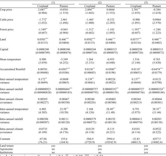
Table 3. Land use equations parameters estimations for 1986-2005 climate variables for BLA in 2006

(1) (2) (3)

Cropland Pasture Cropland Pasture Cropland Pasture

Crop price 2.683*** _{-0.0561 2.804}*** _{0.0664 2.581}** _-0.384

(0.904) (1.519) (1.043) (1.552) (1.035) (1.618)

Cattle price -1.772* _{2.461 -1.465 -0.332 -0.900 0.0964}

(1.032) (1.696) (1.000) (2.285) (1.091) (2.570)

Forest price -1.549** _{-0.865 -1.312}* _{-1.102 -1.393}** _-1.244

(0.687) (0.984) (0.682) (1.093) (0.687) (1.223)

Land 0.0583*** _0.446*** _0.0582*** _0.446*** _0.0573*** _0.446***

(0.0115) (0.0404) (0.0115) (0.0404) (0.0116) (0.0402)

Capital 0.0000240 0.0000306 0.0000244 0.0000315 0.0000250 0.0000313

(0.0000709) (0.0000874) (0.0000716) (0.0000875) (0.0000726) (0.0000872)

Mean temperature 0.980 -5.349 1.264 -0.955 1.516 0.763

(3.039) (6.252) (3.131) (6.040) (3.144) (5.830)

Accumulated Rainfall 0.00701 -0.0307*** _0.0138** _-0.0500** _0.0119* _-0.0474***

(0.00448) (0.0106) (0.00685) (0.0196) (0.00651) (0.0179)

Inter-annual temperature

variance 0.172

** _{-0.0688 0.139}** _{0.00226 0.137}** _-0.0121

(0.0689) (0.0865) (0.0661) (0.0822) (0.0644) (0.0790)

Inter-annual rainfall

variance -0.000000921 0.00000484

*** _{-0.000000757 0.00000352}** _{-0.000000727 0.00000324}** (0.000000828) (0.00000183) (0.000000793) (0.00000150) (0.000000756) (0.00000148)

Inter-annual climate

covariance (0.00227) 0.00265 (0.00330) -0.00467 (0.00224) 0.00246 (0.00306) -0.00402 (0.00213) 0.00244 (0.00301) -0.00444

Intra-annual temperature

variance 6.802 23.58

** _{2.104 28.49}** _{0.791 28.35}**

(4.305) (10.50) (4.126) (11.48) (3.973) (11.44)

Intra-annual rainfall

variance (0.000507) 0.000386 (0.00120) 0.00111 (0.000572) 0.0000379 (0.00138) 0.00192 (0.000574) 0.0000411 (0.00138) 0.00203

Intra-annual climate

covariance -0.0733 (0.109) (0.176) -0.206 -0.0129 (0.118) (0.221) -0.115 (0.114) 0.0181 -0.0522 (0.222)

Constant -47.04 155.6 -504.9 2994.4 -32.83 4357.5

(76.21) (164.8) (3720.9) (18342.9) (4063.5) (18402.6)

Land tenure yes yes yes

Agronomic no yes yes

Institutions no no yes

Standard errors in parentheses: *_{p < 0.1,} **_{p < 0.05,} ***_{p < 0.01.}

32 statistical relationship, the overall pattern within each period appears robust. Climate variables for the 1986-2005 interval have a more consistent relationship with land allocation equations. This is likely to happen for at least two reasons. First, farmers in BLA would take in account climate information from a closer and narrower time horizon. Thus, climate information from 1986-2005 time span presents stronger results in magnitude and statistical significance. Second, remote climate data would be more imprecise than estimates in near past due measurement errors. As a result, estimated coefficients are likely to be biased toward zero. Hence, we chose column 3 in Table 3 as a baseline model. Although there is no consensus in literature regarding time span to retrieve climate variables, our choice agrees with recent structural applications. For instance, Kaminski, Kan, and Fleischer (2012) used an interval of 20 years while Fezzi et al. (2014) used an interval of 30 years.

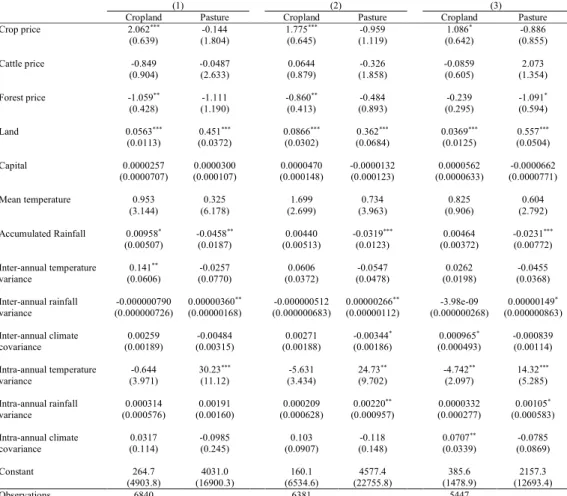
33 baseline model. In fact, accumulated rainfall coefficients are overestimated and inter-annual rainfall variance coefficients are underestimated in the baseline model compared to column 1 in Table 4. Thus, irrigated agriculture does not appear to be a great source of bias for land use estimation in BLA.

Table 4. Land use equations parameters estimations for 1986-2005 climate variables without municipalities with irrigation or without representative farms with few respondents for BLA in 200624

(1) (2) (3)

Cropland Pasture Cropland Pasture Cropland Pasture

Crop price 2.062*** _{-0.144 1.775}*** _{-0.959 1.086}* _-0.886

(0.639) (1.804) (0.645) (1.119) (0.642) (0.855)

Cattle price -0.849 -0.0487 0.0644 -0.326 -0.0859 2.073

(0.904) (2.633) (0.879) (1.858) (0.605) (1.354)

Forest price -1.059** _{-1.111 -0.860}** _{-0.484 -0.239 -1.091}*

(0.428) (1.190) (0.413) (0.893) (0.295) (0.594)

Land 0.0563*** _0.451*** _0.0866*** _0.362*** _0.0369*** _0.557***

(0.0113) (0.0372) (0.0302) (0.0684) (0.0125) (0.0504)

Capital 0.0000257 0.0000300 0.0000470 -0.0000132 0.0000562 -0.0000662

(0.0000707) (0.000107) (0.000148) (0.000123) (0.0000633) (0.0000771)

Mean temperature 0.953 0.325 1.699 0.734 0.825 0.604

(3.144) (6.178) (2.699) (3.963) (0.906) (2.792)

Accumulated Rainfall 0.00958* _-0.0458** _{0.00440 -0.0319}*** _{0.00464 -0.0231}***

(0.00507) (0.0187) (0.00513) (0.0123) (0.00372) (0.00772)

Inter-annual temperature

variance 0.141

** _{-0.0257 0.0606 -0.0547 0.0262 -0.0455}

(0.0606) (0.0770) (0.0372) (0.0478) (0.0198) (0.0368)

Inter-annual rainfall

variance -0.000000790 0.00000360

** _{-0.000000512 0.00000266}** _{-3.98e-09 0.00000149}*

(0.000000726) (0.00000168) (0.000000683) (0.00000112) (0.000000268) (0.000000863)

Inter-annual climate

covariance 0.00259 -0.00484 0.00271 -0.00344

* _0.000965* _-0.000839

(0.00189) (0.00315) (0.00188) (0.00186) (0.000493) (0.00114)

Intra-annual temperature

variance -0.644 30.23

*** _{-5.631 24.73}** _-4.742** _14.32***

(3.971) (11.12) (3.434) (9.702) (2.097) (5.285)

Intra-annual rainfall

variance 0.000314 0.00191 0.000209 0.00220

** _{0.0000332 0.00105}*

(0.000576) (0.00160) (0.000628) (0.000957) (0.000277) (0.000583)

Intra-annual climate

covariance 0.0317 -0.0985 0.103 -0.118 0.0707

** _-0.0785

(0.114) (0.245) (0.0907) (0.148) (0.0339) (0.0869)

Constant 264.7 4031.0 160.1 4577.4 385.6 2157.3

(4903.8) (16900.3) (6534.6) (22755.8) (1478.9) (12693.4)

Observations 6840 6381 5447

(1) Without municipalities with irrigation, (2) without representative farms with less than 15

respondents, and (3) without representative farms with less than 30 respondents. Standard errors in

parentheses: *_{p < 0.1,} **_{p < 0.05,} ***_{p < 0.01.}

34 Another source of bias is measurement errors in dependent variables. If a respondent declared a wrong land use allocation, this error has a greater weight in representative farm with less respondents. The effect of this measurement error tends to zero as the number of respondents tend to infinite within a representative farm. If there is no correlation between measurement errors and explanatory variables, the standard deviations are inflated. If this correlation exists, the estimated coefficients are biased. To verify these possible biases, we estimated the baseline model without representative farms with less than 15 and 30 respondents. The results are in columns 2 and 3 in Table 4, respectively. We lost 708 observations in column 2 and 1642 observation in column 3. Compared to baseline model, accumulated rainfall coefficients decay in columns 2 and 3 in both land use equations. These coefficients are no longer significant for crop equations. Inter-annual temperature variance in cropland equation becomes not significant in columns 2 and 3. There is a reduction in coefficients of inter-annual rainfall variance in pasture equation in both columns. Some coefficients of inter-annual climate covariance, intra-annual temperature variance, intra-annual rainfall variance and intra-annual climate covariance become significant at 5% or 10%. We could not know the extent of the estimation changes are due to reduction of measurement error or to the restricted dataset, but results are qualitative similar to baseline model for accumulated rainfall and inter-annual rainfall variance.