www.atmos-chem-phys.net/14/12701/2014/ doi:10.5194/acp-14-12701-2014
© Author(s) 2014. CC Attribution 3.0 License.
Potential climate forcing of land use and land cover change
D. S. Ward1, N. M. Mahowald1, and S. Kloster2
1Earth and Atmospheric Science, Cornell University, Ithaca, New York, USA
2Land in the Earth System, Max Planck Institute for Meteorology, Hamburg, Germany Correspondence to:D. S. Ward ([email protected])
Received: 13 April 2014 – Published in Atmos. Chem. Phys. Discuss.: 14 May 2014 Revised: 16 October 2014 – Accepted: 5 November 2014 – Published: 3 December 2014
Abstract.Pressure on land resources is expected to increase as global population continues to climb and the world be-comes more affluent, swelling the demand for food. Chang-ing climate may exert additional pressures on natural lands as present-day productive regions may shift, or soil quality may degrade, and the recent rise in demand for biofuels increases competition with edible crops for arable land. Given these projected trends there is a need to understand the global cli-mate impacts of land use and land cover change (LULCC). Here we quantify the climate impacts of global LULCC in terms of modifications to the balance between incoming and outgoing radiation at the top of the atmosphere (radiative forcing, RF) that are caused by changes in long-lived and short-lived greenhouse gas concentrations, aerosol effects, and land surface albedo. We attribute historical changes in terrestrial carbon storage, global fire emissions, secondary organic aerosol emissions, and surface albedo to LULCC us-ing simulations with the Community Land Model version 3.5. These LULCC emissions are combined with estimates of agricultural emissions of important trace gases and min-eral dust in two sets of Community Atmosphere Model sim-ulations to calculate the RF of changes in atmospheric chem-istry and aerosol concentrations attributed to LULCC. With all forcing agents considered together, we show that 40 % (±16 %) of the present-day anthropogenic RF can be at-tributed to LULCC. Changes in the emission of non-CO2
greenhouse gases and aerosols from LULCC enhance the total LULCC RF by a factor of 2 to 3 with respect to the LULCC RF from CO2alone. This enhancement factor also
applies to projected LULCC RF, which we compute for four future scenarios associated with the Representative Concen-tration Pathways. We attribute total RFs between 0.9 and 1.9 W m−2to LULCC for the year 2100 (relative to a prein-dustrial state). To place an upper bound on the potential of
LULCC to alter the global radiation budget, we include a fifth scenario in which all arable land is cultivated by 2100. This theoretical extreme case leads to a LULCC RF of 3.9 W m−2 (±0.9 W m−2), suggesting that not only energy policy but also land policy is necessary to minimize future increases in RF and associated climate changes.
1 Introduction
More than half of the Earth’s land surface has been affected by land use and land cover change (LULCC) activities over the last 300 years, largely from the expansion of agricul-ture (Hurtt et al., 2011), leading to numerous climate im-pacts (Foley et al., 2005). Conversion of land from natural vegetation to agriculture or pasturage releases carbon from vegetation and soils into the atmosphere (Houghton et al., 1983), often quickly through fires, which emit carbon dioxide (CO2), methane (CH4), ozone (O3)-producing compounds,
and aerosols (Randerson et al., 2006). Deforested areas have a diminished capacity to act as a CO2 sink as atmospheric
CO2concentrations increase (Arora and Boer, 2010;
Strass-mann et al., 2008). Furthermore, agriculture and pasturage emits CH4 and nitrous oxide (N2O), accelerates soil
system (Fig. 1), quantified in this study as radiative forcings (RFs).
The global RF and associated climate response attributable to LULCC are often portrayed as a balance between cooling biogeophysical effects (changes in surface energy and water balance) and the warming biogeochemical effect of increases in atmospheric CO2 (e.g., Claussen et al., 2001; Brovkin et
al., 2004; Foley et al., 2005; Bala et al., 2007; Cherubini et al., 2012). Claussen et al. (2001) found that the cooling from biogeophysical effects of land cover change dominated over the warming from associated CO2emissions in high-latitude
regions, where the land may be snow covered for part of the year, whereas tropical LULCC leads to a warming due to a weaker albedo forcing. This regional contrast in the dominant forcing from deforestation also applies to natural forest dis-turbances (O’Halloran et al., 2011). On a global scale, model estimates have shown both canceling climate responses to historical land cover change biogeophysical effects and CO2
emissions (Brovkin et al., 2004; Sitch et al., 2005) and a net warming (0.15◦C) from the same effects (Matthews et al., 2004).
Additional LULCC forcings are often grouped together with fossil fuel burning and other activities for assessment of the total anthropogenic RF (e.g., Forster et al., 2007; Myhre et al., 2013). Nevertheless, there is some recogni-tion of the importance of evaluating emissions of non-CO2
greenhouse gases attributable to LULCC separately from fossil fuel emissions for targeting emission reduction poli-cies (Tubiello et al., 2013). Less attention is given to forc-ings from short-lived atmospheric species that are affected by LULCC. Foley et al. (2005) acknowledge that changes in the concentrations of short-lived species, aerosols and O3,
at-tributable to LULCC are important for air quality assessment but do not estimate the impacts of these species on climate. Unger et al. (2010) partition sources of global, anthropogenic RF into economic sectors, including agriculture. They con-sider non-CO2greenhouse gas and aerosol forcing agents but
only for present-day land use emissions and they do not in-clude land cover change. The full contribution of LULCC to global RF compared to the contribution from other anthro-pogenic activities remains unquantified.
Here we compute the CO2and albedo RF attributable to
global LULCC and compare to previous estimates of these values, but we also compute the forcings from non-CO2
greenhouse gases (CH4, N2O, O3), as well as aerosol effects
(direct, indirect, deposition on snow and ice surfaces). Indi-vidual forcings are computed from the results of terrestrial model simulations forced with historical land cover changes and wood harvesting, and projected land cover changes from five future scenarios. Because the land model used here in-cludes a carbon model, fire module, and emissions of volatile organic compounds, we can uniquely account for the com-plicated interplay between land use and fire (e.g., Marlon et al., 2008; Kloster et al., 2010; Ward et al., 2012). Four of the future scenarios of land cover change correspond
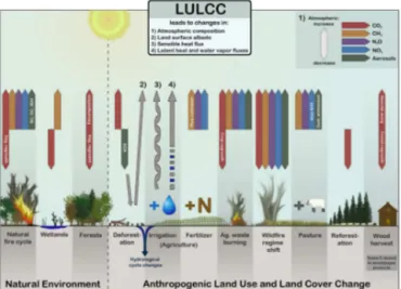
Figure 1.A schematic illustration of the climate impacts of land use and land cover change. See Fig. 2 for a representation of the processes and emissions included in this study.
to the four Representative Concentration Pathways (RCPs) that were developed for the Climate Model Intercomparison Project in preparation for the IPCC 5th assessment report (AR5) (Lawrence et al., 2012; Hurtt et al., 2011; van Vuuren et al., 2011). The low-emissions scenario, RCP2.6, includes widespread proliferation of bioenergy crops (van Vuuren et al., 2007), while RCP4.5 is characterized by global reforesta-tion as a result of carbon credit trading and emission penalties (Wise et al., 2009). The higher emissions scenarios include expansion of crop area at the expense of existing grasslands (RCP6.0; Fujino et al., 2006) or forests (RCP8.5; Riahi et al., 2007; Hurtt et al., 2011). We introduce a fifth, more extreme scenario in which all arable and pasturable land is converted to agricultural land, either for crops or pasture, by the year 2100. This scenario, hereafter referred to as the theoretical extreme case (TEC), was not developed within an integrated modeling framework, and therefore its likelihood of occur-rence given economical and additional environmental con-straints is difficult to judge. Instead, this scenario gives a the-oretical upper bound on LULCC impacts over this century. The range in outcomes for the RF attributable to LULCC based on these five projections strengthens our understanding of the role that LULCC decision making will play in future climate.
2 Overview of methods
Our approach for computing the RFs begins with estimating emissions of trace gases and aerosols from a diverse set of LULCC activities, many of which are illustrated schemati-cally in Fig. 1. For several forcing agents, including CO2, we
attribute the difference in emissions between these simula-tions to LULCC. This general approach, attributing the dif-ferences between the LULCC and no-LULCC environment to the impacts of LULCC, also applies to our calculations of RFs. Our methods for computing these and other emis-sions from LULCC activities, as well as the calculations of changes in atmospheric constituent concentrations and RFs are summarized in this section and schematically in Fig. 2. 2.1 LULCC activities
We model the following LULCC activities with a global terrestrial model: wood harvesting, land cover change, and changes in fire activity, including deforestation fires. Changes in the terrestrial model carbon cycle driven by the historical and projected LULCC are used to derive the RF of surface albedo change, as well as emissions of CO2, SOA,
smoke, and mineral dust from LULCC (Fig. 2). We assem-ble emissions from additional LULCC activities: agricultural waste burning, rice cultivation, fertilizer applications, and livestock pasturage, from available data sets corresponding to the RCP LULCC projections.
Future land cover changes and wood harvesting rate pro-jections have been developed as part of the Coupled Model Intercomparison Project phase 5 (CMIP5) (Taylor et al., 2012) with projections corresponding to each of the four RCP scenarios (Hurtt et al., 2011; van Vuuren et al., 2011). These projections have since been joined to historical recon-structions of land use (Hurtt et al., 2011) and expressed as changes in fractional plant functional types (PFTs) which we use in this study with recently amended wood harvest-ing rates for RCP6.0 and RCP8.5 (Lawrence et al., 2012). Global forest area decreases in all projections between 2010 and 2100 except for RCP4.5, which projects large reforesta-tion efforts (Fig. A1). The loss in forests is accompanied by increases in global crop area in all scenarios except RCP4.5, in which crop area decreases to a level not seen since the 1930s (Fig. A1). Development of PFT changes for the TEC is described in Appendix A.
While we consider this list of activities to be highly clusive, several LULCC activities and processes are not in-cluded in this study, either because they are difficult to prop-erly model or represent as a forcing, or because of a poor level of current understanding of the process. We exclude the impacts of anthropogenic water use, mainly irrigation, on global water vapor concentrations and the associated RF (Boucher et al., 2004). Changes in water use and land use have numerous other implications for the hydrological cycle, including impacts on evapotranspiration, runoff, and wetland extent (Sterling et al., 2013). Related to these effects, the im-pact of land surface albedo changes may be further moder-ated by changes in cloudiness (Lawrence and Chase, 2010), which we did not consider in this analysis. Also, emissions of CH4are tied to the global extent of wetlands, which have
likely changed since preindustrial times (Lehner and Doll,
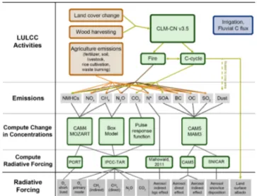
Figure 2.A flow chart summarizing the methodology used in this study to compute the RF of the various forcing agents of LULCC. The colors of the boxes indicate processes that are independent of this study (orange); processes and computational steps that were completed as part of this study (green); and processes that were not included in this study, but are likely important for climate (blue). Acronyms are defined as follows: CLM-CN (Community Land Model with Carbon/Nitrogen cycles) (Oleson et al., 2008; Stöckli et al., 2008), CAM (Community Atmosphere Model) (Gent et al., 2011), MOZART (Model for Ozone and Related Chemical Tracers) (Emmons et al., 2010), PORT (Parallel Offline Radiative Transfer) (Conley et al., 2013), TAR (Third Assessment Report) (Ramaswamy et al., 2001), and SNICAR (Snow Ice and Radiative Aerosol Model) (Flanner and Zender, 2006).∗: total nitrogen (N) includes contributions from NH3, N2O, and NOxemissions.
2004), but the scale and distribution of the change is not yet known well enough to be included in our model setup. We assume that natural CH4emissions remain unchanged from
1850 through 2100 for all scenarios. Finally, there is a source of CO2 from deforestation and forest degradation in
tropi-cal peat swamp forests that has only recently been widely recognized (Hergoualc’h and Verchot, 2011), although it is thought that contributions from this source to current global CO2concentrations are small (Frolking et al., 2011).
2.2 LULCC emissions (computed from CLM)
simulations for each of the LULCC dynamic PFT scenar-ios and compare it to an identical simulation with no PFT changes. All CLM simulations use 1.9◦latitude by 2.5◦ lon-gitude spatial resolution and a 30 min time step.
Spinup of CLM is carried out with year 1850 land cover, which includes some anthropogenic changes. Simulations of historical LULCC run from year 1850 to 2005 and future simulations from year 2006 to 2100. We compute forcings in the year 2010 assuming historical LULCC was extended to 2010 with RCP2.6 land cover changes. We follow the methods of Kloster et al. (2012) for historical and future at-mospheric forcing, including meteorology, CO2
concentra-tions, and N deposition. Twelve future CLM simulations are run, two for each future LULCC scenario (RCP2.6, RCP4.5, RCP6.0, RCP8.5, theoretical extreme case, and No-LULCC) forced from the atmosphere with temperature, precipitation, wind, specific humidity, air pressure, and solar radiation data from the results of two fully coupled CMIP3 simulations. The two sets of atmospheric forcing were selected for their divergent predictions of future temperature and precipitation (Kloster et al., 2012).
2.2.1 Fires
Fire area burned in CLM is controlled by available biomass, fuel moisture, and ignition events, all expressed as prob-abilities, and adjusted by surface wind speeds (Kloster et al., 2010). Fire emissions from the area burned are contin-gent upon the available biomass and are partly determined by PFT-dependent combustion completeness. In addition to wildfires, deforestation fires occur in the model and are repre-sented as an immediate release of a portion of the carbon lost during deforestation. In our analysis, deforestation fires do not impact the overall CO2RF but do speed up the timing of
the release of carbon that would otherwise occur by decom-position. Deforestation fires do, however, contribute small amounts of CH4, N2O, O3precursor gases, and aerosols to
the atmosphere that would not have been released through decomposition.
We attribute a reduction in global burned area, both his-torically and in the future, to LULCC in our simulations (for RCP4.5, which includes large-scale reforestation, the reduc-tion is only a few percent). This result matches our current understanding of the impact of LULCC on wildfires (Kloster et al., 2012; Marlon et al., 2008).
Emissions of trace gases and aerosols by wildfires and de-forestation fires are derived from the CLM simulations of global fire activity. We use 10-year annual average fire car-bon emission output from CLM, corresponding to each anal-ysis year (1850, 2010, 2100), to reduce the influence of in-terannual variability in fires. Emission factors are applied to the carbon emissions from fires to determine the contribution of fires to the various chemical species (see Fig. 2), includ-ing non-methane hydrocarbons (NMHCs), CH4, N2O, NH3,
BC, OC, and SO2 (Kloster et al., 2010; Ward et al., 2012).
The LULCC contribution to global fire emissions of BC and OC is negative in the year 2010 (−13 %), in the year 2100 for all scenarios except for RCP4.5, compared to the no-LULCC CLM realization (Table 1).
2.2.2 Dust emissions
Agricultural activities have been linked to increased wind erosion of soils and greater dust emission in semiarid regions (Ginoux et al., 2012). To address the impact of LULCC on dust emissions we introduce a modified soil erodibility data set for each scenario into simulations with the Community Atmosphere Model (CAM) version 5 (Liu et al., 2011). The model protocol for these simulations is identical to that used to compute the aerosol forcings (see Appendix B5). For each model grid box, a new soil erodibility value is set equal to the sum of the original soil erodibility and the fraction of the grid box that is cultivated land. We then introduce a parameter that weights the cultivated fraction in the soil erodibility compu-tation such that the fraction of the dust flux resulting from cultivation in the year 2000 for eight regions (N. America, S. America, N. Africa, S. Africa, W. Asia, C. Asia, E. Asia, and Australia) is comparable to recently reported, satellite-derived values for each region (Ginoux et al., 2012). The weighting parameter for cultivated land was tuned with three iterations of 4-year global atmospheric model simulations (again using the model setup described in Appendix B5), comparing the results for the tuned and un-tuned soil erodi-bility to the Ginoux et al. (2012) estimates for each region after each iteration. From this tuning we estimate reasonable weighting parameters for the cultivated fraction of land in each of the eight regions. The weighting parameters are ap-plied to the time series of historical and projected crop area to create time series of soil erodibility that are modified by cultivation.
Ginoux et al. (2012) estimate that 25 % of present-day, global dust emissions are caused by anthropogenic activities. We attribute about 20 % of global dust emissions to histori-cal LULCC (Table 1). Once these relationships between land use and dust are developed in the current climate, the natural dust source, along with changes in vegetation and climate are allowed to interact with the prognostic dust scheme to predict changes in dust concentrations (Mahowald et al., 2006; Al-bani et al., 2014). The extreme expansion of crop and pasture area in the TEC leads to more than a tripling of global dust emissions, from natural and human-impacted sources, by the year 2100 using this methodology (Table 1).
2.2.3 SOA emissions
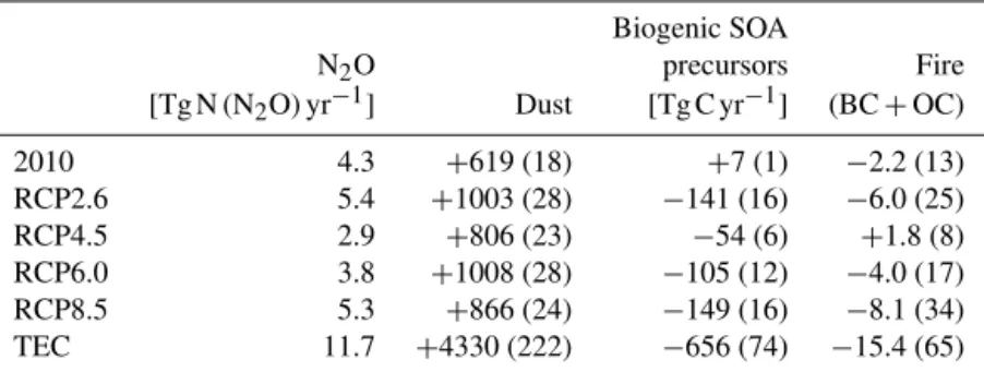
Table 1.Emissions of important aerosol and trace gases attributed to LULCC activities for year 2010 and year 2100 for the listed future scenarios (theoretical extreme case is abbreviated to TEC). Values are given in Tg (species) yr−1except where noted otherwise. Values in parentheses are the percentage change in global emissions attributed to LULCC for the year and scenario listed. Biogenic SOA precursors are considered the sum emissions of biogenic CO, isoprene, monoterpenes, and methanol.
Biogenic SOA
N2O precursors Fire [Tg N(N2O)yr−1] Dust [Tg C yr−1] (BC+OC)
2010 4.3 +619 (18) +7 (1) −2.2 (13) RCP2.6 5.4 +1003 (28) −141 (16) −6.0 (25) RCP4.5 2.9 +806 (23) −54 (6) +1.8 (8) RCP6.0 3.8 +1008 (28) −105 (12) −4.0 (17) RCP8.5 5.3 +866 (24) −149 (16) −8.1 (34) TEC 11.7 +4330 (222) −656 (74) −15.4 (65)
(Guenther et al., 2006) with a forced diurnal cycle for tem-perature and solar radiation (Ashworth et al., 2010). The monthly average LAI outputs from CLM are used for each scenario to produce the biogenic emissions with LAI scaled globally such that predicted year 2000 isoprene emissions match present-day global estimates from Heald et al. (2008). Some biogenic NMHCs, notably monoterpenes and iso-prene, can undergo gas-to-particle phase transitions in the at-mosphere after oxidation (Heald et al., 2008) and contribute to changes in aerosol concentrations. The rate of secondary aerosol production depends on the concentrations of the gas precursors, as well as the oxidation capacity of the tropo-sphere (Shindell et al., 2009). Both criteria are predicted in our atmospheric chemistry model simulations, described in Appendix B2. On a global average, we estimate a negli-gible LULCC-attributed share of biogenic SOA precursors (mainly isoprene) in the year 2010 and attribute larger reduc-tions to projected changes in land cover for the future RCPs between 6 and 16 % (Table 1), similar to the results of Wu et al. (2012) for isoprene plus monoterpene emissions (∼10 % lower with LULCC) between 2000 and 2100 using the IPCC A1B future emissions scenario.
2.2.4 CO2emissions
The anthropogenic contribution to the concentration of at-mospheric CO2, used to compute the RF at years 2010 and
2100, depends on the history of anthropogenic CO2
emis-sions up to that point. We estimate yearly LULCC emisemis-sions to the atmosphere as being equivalent to the global annual change in terrestrial carbon storage due to LULCC. There-fore, sources as well as changes to sinks of CO2associated
with LULCC are accounted for in the CO2emissions. This
approach is most similar to the “D3” group of studies as de-fined by Pongratz et al. (2014), in which simulations with and without LULCC are conducted with identical meteorological and atmospheric CO2forcing.
As noted in previous studies (e.g., Strassmann et al., 2008; Arora and Boer, 2010; Pongratz et al., 2009, 2014), this
methodology does not account for the CO2-fertilization
feed-back in which the CO2attributed to LULCC leads to greater
fertilization of natural and managed vegetation and an en-hanced terrestrial carbon sink. Arora and Boer (2010) show that excluding the CO2-fertilization feedback leads to a form
of “double-counting” land carbon storage and can cause overestimates of 20th century LULCC net carbon flux by about 50 %. A review of the few studies estimating this feed-back gives a range for the overestimate of the net carbon flux from LULCC of 25 to 50 % (Pongratz et al., 2014). How-ever, a recent model intercomparison study suggested that including nitrogen (N) limitation dramatically reduces ter-restrial carbon pool sensitivity to changes in CO2
concen-tration (Arora et al., 2013). Land carbon uptake in coupled models using the CN version of CLM was only 40 % as sen-sitive to changes in CO2concentration and surface
tempera-ture increases (known as the climate change feedback) com-pared to the model used by Arora and Boer (2010). There-fore we adjusted the yearly LULCC net carbon flux down-ward by 20 % to account for the CO2fertilization feedback
and make our calculations of CO2concentration increases
at-tributed to LULCC more consistent with the “E2” group of studies as defined by Pongratz et al. (2014), including Arora and Boer (2010), Strassmann et al. (2008), and Pongratz et al. (2009).
Other model parameters, including aerosol and biogenic NMHC fluxes, depend on LAI, which would also be im-pacted by the different CO2 fertilization. However, due to
the nonlinearity of the aerosol and ozone response, we do not apply an adjustment to these RFs but note here that the magnitude of the year 2010 aerosol, O3, and indirect CH4
RFs may be small overestimates.
that soil carbon is increased following most conversions of natural land to pasture, and decreased following conversions to cropland. Lal (2004) estimates that cultivation has caused the loss of 78±12 PgC from soils since 1850. Modeling studies suggest that LULCC can contribute a net loss of soil carbon globally, from∼13 % of total LULCC carbon emit-ted (Strassmann et al., 2008) to∼37 % (Shevliakova et al., 2009), or a net gain as in Arora and Boer (2010). Recently, Levis et al. (2014) implemented a cultivation parameteriza-tion that includes impacts on soil carbon and found an ad-ditional global flux of 0.4 PgC yr−1 from soils due to crop
management in recent decades.
2.3 LULCC emissions (not computed from CLM) This section describes the sources and accompanying com-putations for LULCC emissions of all relevant trace gas and aerosol species not derived from the CLM simulations in this study (Fig. 2). For non-LULCC-related emissions (such as those from fossil fuel burning) we use the emission invento-ries from the Atmospheric Chemistry and Climate Model In-tercomparison Project (ACCMIP) (Lamarque et al., 2010) for historical time periods, with future emissions from RCP4.5 (Wise et al., 2009). These data sets include emissions of non-methane hydrocarbons (NMHCs), NO, NH3, SO2, and
or-ganic carbon (OC) and black carbon (BC) aerosols. 2.3.1 Agricultural emissions
Agricultural emissions of important trace gas species, such as NH3and N2O, are not simulated by CLM. Therefore,
ad-ditional emissions from LULCC activities associated with agriculture were taken from the integrated assessment model emissions for the different RCPs (e.g., van Vuuren et al., 2011). These activities are fertilizer application, soil modifi-cation, livestock pasturage, rice cultivation, and agricultural waste burning, and we include global emissions of NMHCs, NOx, CH4, NH3, BC, OC, and SO2from LULCC sources.
N2O emissions are not reported by sector for the RCPs and
we compute these separately (Sect. 2.3.2). The four inte-grated assessment models (IAMs) associated with the RCPs for the fifth IPCC assessment report simulate the expansion and contraction of agriculture driven by the demand for food and projected land use policies, such as carbon credits for reforestation or support of expanded biofuel crops (van Vu-uren et al., 2011). The area under cultivation and type of agricultural activities jointly determine the future distribu-tion of agricultural emissions for each projecdistribu-tion (van Vu-uren et al., 2007; Wise et al., 2009; Fujino et al., 2006; Riahi et al., 2007). We use historical agricultural emissions from ACCMIP (Lamarque et al., 2010), which covers the time pe-riod of 1850–2005 and extend the historical emissions with RCP2.6 projected emissions through year 2010 for comput-ing LULCC RFs in the year 2010.
For the TEC, agricultural emissions are derived by scal-ing the RCP8.5 emissions by the difference in cultivated area between the two scenarios in year 2100. First, three latitude band average (−90◦to−30◦,−30◦to 30◦, and 30◦to 90◦ lat-itude) values of emissions of each species per unit cultivated area are computed for RCP8.5, year 2100. Next, the latitude band averages are applied to the theoretical extreme case cul-tivated area in the year 2100, requiring the assumption that the practices and intensity of agriculture in the TEC are the same as in RCP8.5, and only the cultivated area changes. 2.3.2 N2O emissions
N2O has both industrial and agricultural sources, in
addi-tion to a large natural source from soils and oceans. To-tal anthropogenic N2O emissions have been estimated for
the historical time period and projected for RCP4.5 (Mein-shausen et al., 2011a). Additional information regarding nat-ural emissions and also agricultnat-ural emissions is needed to partition the anthropogenic N2O emissions into LULCC and
non-LULCC components and estimate the associated RFs. We follow the methodology of Meinshausen et al. (2011b), in which the N2O budget is balanced for a historical time
period to extract the natural emissions from the total anthro-pogenic emissions. Natural emissions of N2O decrease from
about 11 to 9 TgN (N2O) yr−1using this method between the
years 1850 and 2000. We maintain the year 2000 emissions, 9 TgN (N2O) yr−1, for the years 2000 to 2100. Future land
cover change, particularly the theoretical extreme case, could lead to further reductions in natural N2O emissions through
the year 2100. However, not enough is known about global natural N2O emissions to justify changing the future
emis-sion rate for this analysis (Syakila and Kroeze, 2011). Anthropogenic emissions of N2O have been partitioned
into agricultural (LULCC) and other anthropogenic (primar-ily fossil fuel) sources, which have been further partitioned into animal production and cultivation sources for years prior to 2006 (Syakila and Kroeze, 2011). We compute the global N2O emitted per area covered by crop or pasture in the year
2000 using these estimates. Our estimate for year 2010 N2O
emissions from agriculture, 4.3 TgN (N2O) yr−1, is at the
lower end of previously reported values compiled by Reay et al. (2012), ranging from 4.2 to 7 TgN (N2O) yr−1. The year
2000 ratios of emission per area are applied to future changes in crop or pasture area to compute future LULCC N2O
emis-sions for all scenarios. This assumes no future trends in the rates per cultivated land area of the major agricultural N sources: N fertilizer application and animal waste manage-ment (Syakila and Kroeze, 2011). Our approach results in in-creased N2O emissions from agriculture between years 2010
2.4 Radiative forcing calculations
Radiative forcing (RF) is the change in energy balance at the top of the atmosphere due to a change in a forcing agent, such as an atmospheric greenhouse gas. It is a commonly used metric for comparison of a diverse set of climate forcings and can be used to approximate a global surface tempera-ture response (Forster et al., 2007). The different atmospheric lifetimes of the relevant trace gas and aerosol species (listed in Fig. 2) mean that a single model approach cannot easily capture changes in all the forcing agents (Unger et al., 2010), and therefore a combination of models and methodologies is used here (Fig. 2). Here we summarize the different method-ologies for computing the RFs, while detailed descriptions are given in Appendix B.
We adopt the IPCC AR5 (Myhre et al., 2013) definitions of adjusted RF and effective RF (ERF) and calculate the ad-justed RFs for each forcing agent (ERFs for aerosol forcings) relative to a preindustrial state (year 1850), with modeled radiative transfer or previously published expressions. Our choice of preindustrial reference year is constrained by the available land cover change data sets, which start in 1850. However, large-scale anthropogenic land cover change be-gan centuries before 1850, and preindustrial changes could have an additional impact on present-day climate, perhaps accounting for nearly 10 % of historical anthropogenic global surface temperature change (Pongratz and Caldiera, 2012). In our study, the RF of LULCC relative to the year 1850 is then compared to the RFs of other anthropogenic activ-ities, dominated by fossil fuel burning. RFs due to non-LULCC activities are calculated in this study for RCP4.5 non-LULCC emissions with identical methodology to that used for LULCC emissions. All future LULCC RFs are cal-culated assuming background concentrations of trace gases and aerosols characteristic of RCP4.5. With this approach we can examine the impacts of the range in projected LULCC on RF independent of other anthropogenic activities. However, we are not able to report, for example, the RF of projected LULCC from the RCP8.5 scenario in the context of RCP8.5 fossil fuel emissions. Using a different projection to provide the background concentrations would modify the resulting LULCC RFs.
The RFs of greenhouse gases from LULCC are eas-ily computed from changes in their atmospheric concentra-tions since the preindustrial period. Time-dependent changes in CO2 and N2O concentrations, which are long lived in
the atmosphere, are calculated with simple, pulse-response function and box-model approaches, respectively. To model changes in concentrations of O3, which has a relatively short
atmospheric lifetime, we use the CAM version 4 (Hurrell et al., 2013; Gent et al., 2011) with online chemistry from the Model for Ozone and Related chemical Tracers (MOZART) (Emmons et al., 2010), which simulates all major processes in the photochemical production and loss of O3. Our model
setup also includes changes in O3 deposition rate due to
LULCC impacts on LAI through the vegetation dependence of the dry deposition rate. Results from these simulations also determine changes in the lifetime of CH4due to LULCC
emissions of NMHCs and NOx.
Aerosol chemistry and dynamics are simulated on a global scale using CAM version 5 (Liu et al., 2011) with the three-mode Modal Aerosol Model (MAM3) (Liu et al., 2012), including the two-moment microphysical scheme (Morri-son and Gettelman, 2008) and aerosol–cloud interactions for stratiform clouds. Since models generally disagree on the magnitude of the aerosol effects, we use the IPCC-AR5 cen-tral estimate aerosol direct and indirect ERFs for the year 2011 to estimate the total anthropogenic aerosol forcing in the year 2010 and use our model results to determine the proportion of the total anthropogenic aerosols effects due to LULCC. We then apply the same scaling to the aerosol effects in all future scenarios. The impacts of the LULCC aerosol emissions, both direct effects and indirect effects on clouds, are diagnosed online within CAM5. We do not at-tempt to isolate the RF of aerosols from quick-responding cloud feedbacks within the model, and the computed forcings that include these feedbacks are more appropriately referred to as effective radiative forcings (ERFs). For computing a to-tal forcing from LULCC we include the aerosol ERFs with the RFs of the remaining forcing agents.
LULCC activities change vegetation cover and type, af-fect forest canopy coverage, and alter wildfire activity, all of which impact land surface albedo. We compute these im-pacts using output from the CLM simulations with and with-out LULCC (Sect. 2.2). Monthly averages for solar radiation incident upon the surface (after accounting for attenuation by monthly average cloud cover) are multiplied by the surface albedo with LULCC and without LULCC for each model grid point. The RF equals the global annual average differ-ence between the outgoing solar radiation with LULCC and without LULCC.
2.4.1 Uncertainty
The uncertainty in these RF estimates arises largely from the uncertainty in modeling the effects of aerosols and model-ing the impacts of climate, CO2 changes, and LULCC on
In addition to the uncertainties, there are a few shortcom-ings inherent in our approach. We do not include many bio-geophysical effects of LULCC, such as changes to surface latent and sensible heat fluxes and to the hydrological cy-cle, that impact climate (Defries et al., 2002; Feddema et al., 2005; Brovkin et al., 2006; Pitman et al., 2009; Lawrence and Chase, 2010). In general, while important for local or regional climate especially in the tropics (Strengers et al., 2010), these effects are considered minor on a global scale (Lawrence and Chase, 2010) and are difficult to quantify using the RF concept (Pielke et al., 2002). For the calcula-tion of the many forcing agents that we do consider, our ap-proach is to treat each forcing separately, which could lead to differences in RFs between agents that are due partly to methodology. For example, land cover changes and agricul-tural emissions were developed jointly for each of the RCPs, but for use in terrestrial models, including CLM, the land cover change projections were altered (Di Vittorio et al., 2014). This leads to inconsistent storylines between future emissions computed by CLM (Sect. 2.2) and those taken directly from the RCP integrated assessment model output (Sect. 2.3.1). Therefore, it is important to view the future RFs computed here as comprising a broad range in possi-ble outcomes, extended with the TEC, as opposed to pre-cise results corresponding to specific storylines for the fu-ture. Finally, the inhomogeneous distribution of forcing from surface albedo changes and short-lived trace gas and aerosol species could lead to non-additive (A. D. Jones et al., 2013) and highly variable local climate responses (Lawrence et al., 2012). Therefore, we use the RF for our assessment of global-scale climate impacts and acknowledge the limits of the RF concept for predicting the diverse and often local im-pacts of land use (Betts, 2008; Runyan et al., 2012).
3 Results
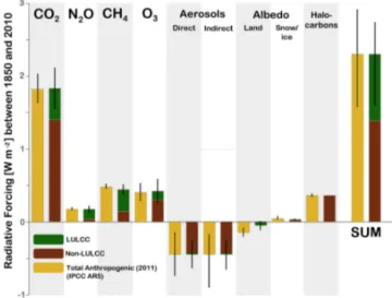
3.1 Land use impacts on present-day radiative forcing We estimate a RF in the year 2010 from LULCC of 0.9±0.5 W m−2, 40 % (
±16 %) of the present-day total thropogenic RF (Fig. 3, Table 2). By separating the total an-thropogenic RF (sum of LULCC and other anan-thropogenic activities) into contributions by forcing agent, we can com-pare our calculations to the central estimates of Myhre et al. (2013) (Fig. 3) and the reported RFs of van Vuuren et al. (2011) (Table 3). Our calculations of the total, present-day, anthropogenic RF correspond closely to the van Vuuren et al. (2011) values.
The major contributors to the present-day LULCC RF are associated increases in atmospheric CO2 and CH4.
Defor-estation, driven largely by the demand for additional agri-cultural land, leads to an estimated net decrease in global forest area of roughly 5.5 million km−2 from 1850 to 2010
(Lawrence et al., 2012; Fig. A1) and a transfer of carbon
Figure 3.RFs for LULCC and other anthropogenic impacts esti-mated by this study for the year 2010 referenced to the year 1850. Total anthropogenic RF from the IPCC AR5 (Myhre et al., 2013) are shown for comparison (yellow). Error lines represent 1σ uncer-tainties in total anthropogenic RF for the IPCC bars and 1σ uncer-tainties in LULCC RFs as computed in this study (green bars; data given in Table 2). The “SUM” bars show the total RF when all forc-ing agents are combined. Note that aerosol ERFs are scaled to IPCC AR5 values, as explained in the main text.
from the terrestrial biosphere into the atmosphere. Past stud-ies report a LULCC contribution to current CO2
concentra-tions (either year 2000 or 2005) of 26 ppm (Matthews et al., 2004), 22 to 43 ppm (Brovkin et al., 2004),∼45 ppm (Strass-mann et al., 2008), and 17 ppm (Arora and Boer, 2010). Af-ter adjusting for the CO2fertilization feedback, we estimate
a LULCC contribution of 28 ppm CO2 in the year 2010.
Our approach results in a year 2010 CO2 concentration of
399 ppm (285 ppm preindustrial, 86 ppm fossil fuels, 28 ppm LULCC), which overshoots the observed change in CO2over
the same period by about 10 % but is within the range of values from the CMIP5 fully coupled climate model exper-iment: 368 to 403 ppm in 2005 (Friedlingstein et al., 2013). The overestimate is in this case attributable to uncertainty in the total LULCC CO2emissions and uncertainty regarding
the airborne fraction of historical emissions.
Present-day LULCC and non-LULCC anthropogenic ac-tivities each emit close to 150 Tg CH4annually (van Vuuren
et al., 2007), yet the RF from LULCC CH4is roughly
dou-ble the RF from non-LULCC CH4(Fig. 3). The RF of
non-LULCC CH4 is diminished relative to LULCC CH4by the
concurrent emission of non-LULCC NOx, which leads to
greater tropospheric ozone (O3)production, an increase in
the oxidation capacity of the troposphere, and, as a result, a 20 % reduction in CH4lifetime with respect to removal by
reaction with OH (Appendix B3).
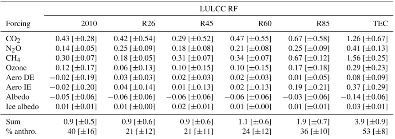
Table 2.LULCC RF values and uncertainties for year 2010 and all future scenarios (year 2100) relative to the year 1850. Sum RFs are the total of all forcing agents and have been rounded to the nearest 0.1 W m−2. The theoretical extreme case is abbreviated to “TEC”.
LULCC RF
Forcing 2010 R26 R45 R60 R85 TEC
CO2 0.43 [±0.28] 0.42 [±0.54] 0.29 [±0.52] 0.47 [±0.55] 0.67 [±0.58] 1.26 [±0.67] N2O 0.14 [±0.05] 0.25 [±0.09] 0.18 [±0.08] 0.21 [±0.08] 0.25 [±0.09] 0.41 [±0.13]
CH4 0.30 [±0.07] 0.18 [±0.05] 0.31 [±0.07] 0.34 [±0.07] 0.67 [±0.12] 1.56 [±0.25] Ozone 0.12 [±0.17] 0.06 [±0.13] 0.10 [±0.15] 0.10 [±0.15] 0.17 [±0.18] 0.29 [±0.23] Aero DE −0.02 [±0.19] 0.03 [±0.03] 0.02 [±0.03] 0.02 [±0.03] 0.01 [±0.05] 0.08 [±0.09] Aero IE −0.02 [±0.20] 0.04 [±0.14] 0.01 [±0.13] 0.02 [±0.13] 0.19 [±0.21] 0.37 [±0.29] Albedo −0.05 [±0.06] −0.06 [±0.06] −0.06 [±0.06] −0.06 [±0.06] −0.03 [±0.06] −0.14 [±0.06] Ice albedo 0.01 [±0.01] 0.01 [±0.00] 0.02 [±0.01] 0.01 [±0.00] 0.01 [±0.01] 0.03 [±0.01]
Sum 0.9 [±0.5] 0.9 [±0.6] 0.9 [±0.6] 1.1 [±0.6] 1.9 [±0.7] 3.9 [±0.9] % anthro. 40 [±16] 21 [±12] 21 [±11] 24 [±12] 36 [±10] 53 [±8]
Table 3.Radiative forcings (W m−2)for the year 2010 and the year 2100 compared to Myrhe et al. (2013) and van Vuuren et al. (2011),
respectively. For year 2100 we show the RF from RCP4.5 scenario emissions (referenced to year 1850) estimated from the modeling results in this study and from van Vuuren et al. (2011).
Total
2010 LULCC Non-LULCC anthro. Myhre et al. (2013)
Total 0.91 1.39 2.3 2.22
CO2 0.43 1.4 1.83 1.82
CH4 0.3 0.14 0.44 0.48
N2O 0.14 0.03 0.17 0.17
Halocarbons 0 0.36 0.36 0.36 Aerosols/O3/alb∗ 0.04 −0.54 −0.5 −0.61
2100-RCP4.5 van Vuuren et al. (2011)
Total 0.92 3.49 4.41 4.14
CO2 0.29 3.17 3.46 3.47
CH4 0.31 0.12 0.43 0.37
N2O 0.18 0.12 0.3 0.31
Halocarbons 0 0.18 0.18 0.18 Aerosols/O3/alb∗ 0.14 −0.1 0.04 −0.19
∗This sum RF includes aerosols (direct effects, indirect effects on clouds, and deposition onto snow/ice surfaces), tropospheric O3, and forcing from surface albedo changes.
304 Tg in 2010, when all anthropogenic activities are in-cluded. The O3 increase of 112 Tg falls within the range of
previous estimates (Lamarque et al., 2005). Here we separate the increase in O3concentrations into a non-LULCC
contri-bution, 87 %, and a LULCC contricontri-bution, 13 %. The large non-LULCC contribution is attributable to additional O3
for-mation from NOxemissions from fossil fuel burning sources.
The contribution of LULCC to changes in O3combines
sev-eral competing effects (Ganzeveld et al., 2010), including at-tributed changes in biogenic emissions of volatile organic compounds (virtually no contribution by historical LULCC on a global average) and reductions in emissions from wild-fires (Table 1). The increase in tropospheric O3from LULCC
is partially compensated for by a slight increase in the dry
de-position of O3with LULCC (6 %) between 1850 and 2010
as a result of the LULCC-enhanced O3 concentration and
despite the decrease in O3 removal efficiency in deforested
areas, similar to the findings of Ganzeveld et al. (2010). The small contribution of LULCC to global “short-lived” O3
con-centrations is augmented by additional O3(2.5 DU in 2010)
produced in response to long-term increases in CH4
(pri-mary mode response, Appendix B2). The additional O3from
this response accounts for 60 % of the LULCC O3 RF of
0.12 W m−2in 2010. The primary mode response O 3is less
important for non-LULCC activities because of the smaller CH4contribution from these activities.
We assume that long-lived greenhouse gases, i.e., CO2,
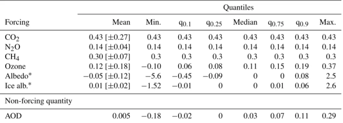
Table 4.Quantiles of the spatial distribution of the different forcings from historical LULCC (assessed in 2010) when represented as a probability density function. The grid spacing is 1.9◦latitude by 2.5◦longitude. Note that we show aerosol optical depth (AOD) in place of the aerosol forcings since the distribution of these forcings includes variability in cloud properties that are not directly attributable to changes in aerosols at this grid spacing.
Quantiles
Forcing Mean Min. q0.1 q0.25 Median q0.75 q0.9 Max.
CO2 0.43 [±0.27] 0.43 0.43 0.43 0.43 0.43 0.43 0.43 N2O 0.14 [±0.04] 0.14 0.14 0.14 0.14 0.14 0.14 0.14
CH4 0.30 [±0.07] 0.3 0.3 0.3 0.3 0.3 0.3 0.3
Ozone 0.12 [±0.18] −0.10 0.06 0.08 0.11 0.15 0.19 0.37 Albedo∗ −0.05 [±0.12] −5.6 −0.45 −0.09 0 0 0.08 2.5 Ice alb.∗ 0.01 [±0.02] −1.52 −0.01 0 0 0.01 0.06 2.6
Non-forcing quantity
AOD 0.005 −0.18 −0.02 0 0.03 0.07 0.11 0.29
∗The spatial distribution of the RF from albedo changes is computed only for land points.
centuries, are sufficiently well mixed in the atmosphere that the forcing from these gases is spatially homogeneous (Table 4). The lifetime of tropospheric O3 is considerably
shorter, on the order of weeks, meaning concentrations can vary spatially, becoming higher near areas of O3
produc-tion and remaining below the global average in remote re-gions away from areas of O3production. The RF varies in
space with the concentration, although these heterogeneities are moderate for O3. The RF at 80 % of grid points is within ±0.07 W m−2of the global mean RF (Table 4).
While the positive RF from non-LULCC greenhouse gas emissions is offset to some extent by concurrent emissions of aerosols, LULCC contributes both increases and decreases in aerosol emissions resulting in nearly neutral aerosol RFs for the present day (Fig. 3). These opposing contributions to aerosol emissions are evident in the spatial variability in AOD attributable to historical LULCC, ranging between −0.18 and 0.29 (Table 4). Global average aerosol optical depth (AOD) is greater in 2010 and in 2100 for the RCP4.5, RCP6.0, and TEC scenarios when LULCC emissions are in-cluded, and lower for RCP2.6 and RCP8.5 scenarios, but in all cases the attributed share of LULCC is less than 0.01. The RF from aerosol deposition onto snow and ice surfaces is negligible on a global average (0.01 W m−2 for
histori-cal LULCC) but exceeds±1 W m−2in some locations
(Ta-ble 4). We also consider the impacts of aerosols and trace gas species on atmospheric CO2due to bio-fertilization by
deposition of P, Fe, and N emitted from fires, and N from agriculture (NH3, NOx, N2O). For present-day emissions of
these species from LULCC activities (and land cover change impacts on fires), the drawdown of CO2, enhanced
particu-larly by agricultural emissions of N, leads to a negative RF of−0.10 W m−2that nearly compensates for the positive RF
from the greenhouse effect of agricultural N2O emissions
(0.14 W m−2), a noteworthy aspect of agricultural emissions
that was also suggested by Zaehle et al. (2011).
Estimates for the global RF from albedo changes range from−0.10 (Skeie et al., 2011) to−0.28 W m−2(Lawrence
et al., 2012), with a substantial percentage, potentially 25 %, caused by preindustrial LULCC (Pongratz et al., 2009). Further estimates (Betts, 2001; Betts et al., 2007; Davin et al., 2007) fall near the IPCC AR5 central estimate of −0.15 W m−2 (Myhre et al., 2013). The RF from albedo
changes is near zero in most locations but has a high mag-nitude, up to 5 W m−2, in some localities on an annual
aver-age (Table 4), similar to the findings of Betts et al. (2007). Our estimate for the global RF from historical land sur-face albedo change, −0.05 W m−2, is at the higher end of the range of previously published estimates, yet still within the 90 % confidence interval around the central estimate of Myhre et al. (2013). Reductions in fire area burned that re-sult from historical LULCC act to decrease the magnitude of the surface albedo change forcing, although by less than 0.01 W m−2 for the present day. The use of a less altered,
more natural background state than our year 1850 landscape would likely increase the magnitude of this forcing (Sitch et al., 2005; Pongratz et al., 2009).
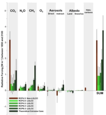
3.2 Future land use impacts on radiative forcing In the year 2100 the RF attributable to anthropogenic LULCC, as projected by the RCPs, ranges between 0.9 and 1.9 W m−2(Fig. 4), although, as a percentage of the projected
LULCC RF that is double the average of the other three RCP scenarios. The difference between RCP8.5 and the other sce-narios suggests that decisions regarding global land policy similar to those used to develop the RCPs could reduce or increase global anthropogenic RF by 1 W m−2by 2100.
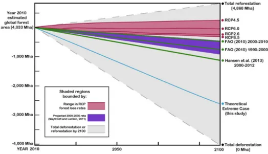
The LULCC projections for all four RCP scenarios include future decreases in global deforestation rates compared to re-cent historical rates (Fig. 5). A rere-cent satellite assessment of global forest area gain and loss reported a global forest loss rate of 12.5 Mha yr−1between 2000 and 2012 (Hansen et al.,
2013), suggesting the census-reported rates for 2000 to 2010 (FAO, 2010) may be estimating less deforestation than is re-ally occurring. If recent rates of observed forest area change persist, the global forest area projected in all four RCP sce-narios by Hurtt et al. (2011) will become overestimates in the near future, especially in RCP4.5 and RCP6.0. More extreme land use scenarios are plausible, and would have a larger ef-fect on climate. The theoretical extreme case, in which all arable land is converted to agricultural land and all remain-ing land that is pasturable is converted to grasses by the year 2100, does not take some important agricultural factors, such as changes in crop yields and per capita caloric intake, into account, but was created to represent a limit to cropland ex-pansion on Earth. Since we designate arable land using a measure of climate suitability (Appendix A), following Ra-mankutty et al. (2002), crop area could conceivably expand beyond this limit with the use of irrigation. In fact, areas of South Asia currently support more agriculture than estimates of climate suitability suggest they should (Ramankutty et al., 2002).
In the theoretical extreme case, crop area roughly doubles by the year 2050, and continues to increase at the same rate to 2100. The rate of deforestation required to accommodate the expanded agriculture is 3 times greater than upper estimates from the RCPs for year 2000–2030 forest loss (Fig. 5), re-sulting in the near-complete removal of tropical forests by the year 2100 (Fig. A2) and a global release of ∼500 PgC from vegetation to the atmosphere. Loss of soil carbon of-ten accompanies forest conversion to crops or grasses (Lal, 2004), but this process is not well simulated in this genera-tion of terrestrial models. House et al. (2002) estimate terres-trial carbon loss from a complete deforestation to be between 450 and 820 PgC, with much of the uncertainty in the range due to different estimates of carbon loss from soils. The ver-sion and configuration of CLM used in this study does not include the process of carbon loss from soils from cultiva-tion. Still, loss of carbon from vegetation alone in the theo-retical extreme case corresponds to roughly two-thirds of the value of the proven reserves of fossil fuels (760 PgC) (Mein-shausen et al., 2009). The substantial loss of terrestrial car-bon to the atmosphere in the theoretical extreme case leads to a RF of 1.3 W m−2for CO
2(Fig. 4). The magnitudes of all
other forcing agents are enhanced in this scenario, leading to a sum RF of 3.9±0.9 W m−2at the year 2100.
Figure 4.RF for all LULCC and non-LULCC anthropogenic im-pacts (RCP4.5 Non-LULCC) estimated by this study for the year 2100, referenced to the year 1850. Error bars show 1σuncertainties as computed in this study (Table 2). The “SUM” bars show the total RF when all forcing agents are considered.
3.3 Enhancement of land use CO2radiative forcing On average over all converted land types and land manage-ment histories, CO2 RF from LULCC is enhanced by the
accompanying (although not necessarily concurrent) emis-sions of non-CO2greenhouse gases and aerosols, such that
the total RF is 2 to 3 times that of the CO2alone. For
exam-ple, we estimate the net carbon flux from LULCC between 1850 and 2010 to be 140 PgC, leading to a RF from CO2
of∼0.4 W m−2 in 2010, or about half of the total LULCC
RF. In contrast, for other anthropogenic activities the RF from CO2 and the total RF are roughly equal (Figs. 3, 4).
Therefore, while LULCC accounted for about 20 % of an-thropogenic CO2-equivalent emissions in 2010 (Tubiello et
al., 2013), its contribution to the anthropogenic RF is 40 % (±16 %). We can express this enhancement factor as the ra-tio of the sum RF to the CO2 RF for LULCC, divided by
the same ratio for other anthropogenic activities (FF+), or E=(RFsum/RFCO2)LULCC/(RFsum/RFCO2)FF+. For all future LULCC scenarios the enhancement factor is between 2.0 and 2.9 (Table 5). We compute the maximum enhance-ment of the CO2 RF for the RCP4.5 scenario (E=2.9). In
the development of the RCP4.5 scenario, international car-bon trading incentivizes preservation of forests and reforesta-tion, which reduces CO2emissions and the resulting CO2RF
Figure 5.Comparison of projected annual rates of forest area change. Colored lines and shading represent the change in global forest area between 2010 and 2100 for the Representative Concentration Pathways (red) and the theoretical extreme case (light blue). The grey shaded region is bounded by the annual rate of forest area change required to completely reforest to the estimated prehistoric forest area (Pongratz et al., 2008), or remove all forests by year 2100. Reported and projected forest area change from Meyfroidt and Lambin (2011) (purple) and FAO (2010) and Hansen et al. (2013) (green) are depicted as constant rates through year 2100 to show the result if these rates were sustained.
Table 5.Enhancement of CO2RF by other forcing agents for LULCC and non-LULCC activities. RFs are given in units of W m−2.
LULCC Non-LULCCa
Scenario CO2 RF TOTAL RF CO2 RF TOTAL RF Enhancementb
2010 0.43 0.91 1.4 1.39 2.1 (+1.0,−0.5) RCP2.6 0.42 0.93 3.17 3.49 2.0 (+1.4,−0.7) RCP4.5 0.29 0.92 3.17 3.49 2.9 (+2.6,−1.6) RCP6.0 0.47 1.11 3.17 3.49 2.1 (+1.5,−0.7) RCP8.5 0.67 1.94 3.17 3.49 2.6 (+1.8,−0.8) TECc 1.26 3.86 3.17 3.49 2.8 (+1.3,−0.6)
aOther anthropogenic activities, dominated by fossil fuel burning, and including the aerosol effects RFs from
the IPCC AR5 (Myhre et al., 2013).bEnhancement is defined as the ratio of total RF to CO2RF for LULCC
divided by the ratio of total RF to CO2RF for FF+.cTheoretical extreme case.
The uncertainties in this factor (computed using the Monte Carlo method as described in Appendix C3) are large but suggest that the enhancement is unlikely to be less than 1.3 for the year 2010 or any of the given future scenarios. Val-ues above 4.0 for the enhancement factor are within the un-certainty range for the RCP4.5, RCP8.5, and TEC scenarios. The large enhancement factors for the RCP8.5 and TEC sce-narios result mainly from the substantial CH4RF relative to
the CO2RF. For RCP4.5, this is a reflection of the low CO2
RF attributed to LULCC and relatively high total RF with contributions from all other non-CO2greenhouse gases. The
aerosol forcings play a minor role in the sum RF attributed to LULCC but impact the enhancement factor by reducing the non-LULCC forcing considerably. The aerosol ERFs are the source of much of the uncertainty surrounding the en-hancement factor. Since the RF calculations presented here
are within uncertainty estimates across many models and es-timates (Fig. 3), it is likely that other models or approaches would obtain similar results if the same processes and activ-ities were considered. We do not expect that the LULCC ac-tivities and biogeophysical forcings that we exclude from this study would have a substantial impact on the enhancement as these forcings have been shown to be small when consid-ered on a global scale (Lawrence and Chase, 2010). Includ-ing model representation of LULCC impacts on soil carbon could increase the CO2 and total RF attributed to LULCC
4 Conclusions
Effective strategies for mitigation of human impacts on global climate require an understanding of the major sources of those impacts (Unger et al., 2010). Anthropogenic land use and changes to land cover have long been recognized as important contributors to global climate forcing (Feddema et al., 2005), and yet most studies on this topic focus on either land use (e.g., Unger et al., 2010) or land cover change (e.g., Davin et al., 2007; Pongratz et al., 2009), but not both. In this study we compute the fraction of anthropogenic RF that is attributable to LULCC activities including a more compre-hensive range of forcing agents.
Current estimates of the net LULCC carbon flux between 1850 and 2000 are between 108 and 188 PgC (Houghton, 2010), while here we estimate 131 PgC. Estimates from this study using the future scenarios analyzed in the IPCC (the Representative Concentration Pathway, RCP, scenarios) sug-gest between 20 and 210 PgC carbon will be released, con-sistent with Strassmann et al. (2008), and at the higher end of the model range reported by Brovkin et al. (2013). Our model underpredicts the uptake of land carbon relative to other models (e.g Arora et al., 2013), and unlike other esti-mates includes the explicit interplay between changes in land use and fires (e.g., Marlon et al., 2008; Kloster et al., 2010). The RCP scenarios were designed to cover a diverse set of pathways and create a broad range in possible outcomes for the next century (Moss et al., 2010). Given that the RCP sce-narios all project decreases in global forest area loss rates in the 21st century relative to current rates, these scenarios are likely to be lower bounds on deforestation rates in the future (Fig. 5). To explore higher rates of global forest loss and crop and pasture expansions, we introduce a theoretical extreme case, in which all the arable land is converted to agriculture and pasture usage by 2100. Since the rates of deforestation in this scenario are higher than current rates, this scenario is an upper bound on what could occur. With the intense pressures on land inherent to this scenario, we calculate that between 590 and 700 PgC would be released from LULCC in this cen-tury.
We find that the total RF contributed by LULCC is 2 to 3 times the RF from CO2alone when additional positive
forc-ings from non-CO2 greenhouse gases and relatively small
forcings from aerosols and surface albedo are considered. The RF of other anthropogenic activities (largely fossil fuels) in 2010 and in 2100 (RCP4.5), relative to 1850, includes a large magnitude negative aerosol forcing that offsets enough of the warming contribution from greenhouse gases that the total RF matches closely with the RF from CO2. The result
of this enhancement of the LULCC RF with respect to its CO2 emissions, and lack of enhancement of the other
an-thropogenic activities RF, is a 40 % LULCC contribution to present-day anthropogenic RF, a substantially larger percent-age that is deduced from greenhouse gas emissions alone (Tubiello et al., 2013). The percentage of anthropogenic RF
attributable to LULCC activities is likely to decrease in the future, even as the magnitude of the RF could increase by up to 1.0 W m−2from 2010 to 2100. The lifetime and
distri-bution of short-lived species makes simplification difficult in terms of equating CO2RF to other constituents (Shine et al.,
2007), but simple approaches of controlling cumulative car-bon (Allen et al., 2009) should account for the 2 to 3 times enhancement of the LULCC RF over long time periods per unit CO2emitted relative to other sources of CO2.
Including forcings from aerosols in our assessment, while only slightly affecting the mean estimate of the total LULCC RF, greatly increases the uncertainty in the estimate. Much of the uncertainty arises from the simulation of aerosol–cloud interactions and the indirect effect for which very little model consensus exists on a global scale (Forster et al., 2007). In addition to these uncertainties, the perturbations of natural aerosol emissions by LULCC activities (mineral dust, SOA, wildfire smoke) are only beginning to be better understood on a global scale (Ginoux et al., 2012; Ganzeveld et al., 2010). Further research into the sources and lifetimes of nat-ural aerosols, as well as anthropogenic impacts on their emis-sions, could efficiently reduce our uncertainty in the contri-bution of LULCC to global RF.
While it is likely that advances in, and proliferation of, agricultural technologies will be sufficient to meet global food demand without such an extreme increase in crop and pasture area, investment in foreign lands for agriculture, as a cost-effective alternative to intensification of existing agri-culture, may be hastening the conversion of unprotected nat-ural lands (Rulli et al., 2013). Given the huge potential for climate impacts from LULCC in this century, estimated here to be 3.9±0.9 W m−2at the maximum, similar to some
Appendix A: Crop suitability calculations for theoretical extreme case
To estimate the maximum extent of crop and pasture for the theoretical extreme future scenario requires criteria that mea-sure the potential of a land area to support agriculture. We follow the methodology of Ramankutty et al. (2002) to define the suitability of the climate and soil properties at model grid point locations for crops or pasture. In that study the authors define suitability based on the growing degree days, mois-ture index, soil organic carbon content, and soil pH that are characteristic of present-day agricultural areas. Areas with a long enough growing season and sufficient water resources to support present-day crops, without irrigation (which is not included in their analysis), are considered suitable based on climate. For both soil organic carbon content and soil pH the authors find an ideal range of values that support agriculture and categorize areas that meet the criteria as suitable based on the soil. We repeat their analysis with temperature and precipitation data from the Climatic Research Unit TS3.10 data set (Harris et al., 2014), soil data from the International Soil Reference and Information Centre – World Soil Infor-mation database (Batjes, 2005), and a simplified moisture in-dex (Willmott and Feddema, 1992).
In this approach, sigmoidal functions are fit to probability density functions of grid box fractional crop area and four environmental factors: growing degree days (GDD), mois-ture index, soil pH, and soil organic carbon density. These functions describe where crops grow in today’s world and how well they grow there. The functions are then applied to current global climate and soil data sets to identify areas that could support crops but have yet to, and also some areas where crops outdo their potential based on the local climate and soil, usually due to irrigation.
We use the Ramankutty et al. (2002) definitions for soil pH; soil carbon, defined as the mass of carbon per meter squared in the top 30 cm of the non-gravel soil; and GDD, defined as the number of◦C by which daily mean tempera-ture exceeds 5◦C.
For the moisture index we use the climate moisture index (CMI) (Willmott and Feddema, 1992) which is defined using precipitation,P, and potential evaporation, PE, data as
CMI=1−PE/P when P ≥PE (A1)
CMI=P /PPE−1 when P <PE
CMI=0 when P =PE=0.
We use 1979–2009 averages for climate variables and year 2000 crop area data (Ramankutty et al., 2008). For fitting the individual sigmoidal curves, we restrict the data to only those points that are otherwise optimal for crops, as in Ramankutty et al. (2002). For example, when fitting the CMI data, we restrict the crop area data to regions where the GDD, soil carbon, and soil pH support crops. This isolates grid points that could be CMI limited.
Figure A1. Change in global total(a) forest and(b) crop areal coverage with time for historical and Representative Concentration Pathway scenarios (Lawrence et al., 2012) and the theoretical ex-treme case (TEC, green).
Following Ramankutty et al. (2002), we fit a single sig-moidal curve to the GDD data and the CMI data, a double sigmoidal curve to the soil carbon data, and explicitly de-fine a pH limit function. The expressions for these functions from Ramankutty et al. (2002) are given below with new co-efficients computed for our study:
f1(GDD)=
1
1+ea(b−GDD); (A2)
f2(α)=
1
1+ec(d−α), (A3)
wherea=0.0037,b=1502,c=10.16, andd=0.3544; g1(Csoil)=
a
1+eb(c−Csoil)
a
1+ed(h−Csoil), (A4) where a=22.09, b=3.759, c=1.839, d=0.0564, and h=106.5;
g2 pHsoil
=
−1.64+0.41 pHsoil if pHsoil≤6.5 1 if 6.5<pHsoil<8 1−2 pHsoil−8
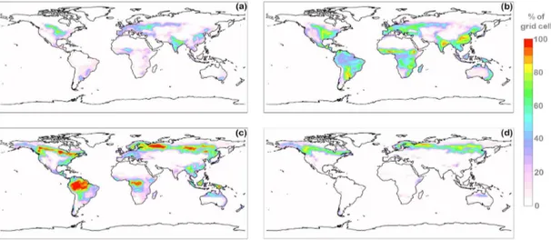
Figure A2.Percent of grid box area consisting of(a)year 2010 crops,(b)potential crops based on climate and soil suitability,(c)year 2010 forests, and(d)year 2100 forests in the theoretical extreme case.
suitability index and the product of thegfunctions gives the soil suitability index. Natural land that is “suitable” for crops based on these criteria is converted to cropland (on a linear year-to-year basis) between years 2006 and 2100. We assume area that is suitable for crops based on climate, but not soil characteristics, can support grass and is used for pasturing animals. This assumption leads to the replacing of most trop-ical forests by crops or grasslands. The global potential crop area computed here for present-day climate is 4180 Mha and the potential pasture area is 3110 Mha, compared to reported year 2010 utilized areas of 1570 Mha for crops and 2030 Mha for pasture (Hurtt et al., 2011). Published estimates of poten-tial crop area range from 1552 to 5131 Mha (Eitelberg et al., 2014). Our estimate for potential crop area would be classi-fied as “high” within this range (Eitelberg et al., 2014), most similar to the results of Bruinsma (2003).
Since the potential crop area depends on climate, it is likely to change in the future. One estimate, using a business-as-usual greenhouse gas emissions scenario, yields a 16 % in-crease of the 1961–1990 potential crop area by 2070–2099, mainly in high latitudes (Ramankutty et al., 2002). We did not include climate-dependent trends in potential crop area in this study but note here that doing so may increase the year 2100 RF of the theoretical extreme case LULCC.
The PFT time series for the theoretical extreme case is put together as follows. First, the potential crop area and poten-tial pasture area are used to give the year 2100 crop area and minimum grassland area, respectively. Crop area is increased linearly starting in year 2006 at the expense of grassland first, then shrubs, then forest area. Pasture is increased at the ex-pense of shrubs, then forest area. Different PFTs within those general categories are lost or gained in proportion to their year 2006 fractions. In this scenario, global crop area in-creases 200 % with substantial expansion into tropical Africa and South America, and southeast Asia (Figs. A1, A2). The
expansion of crops and pasture into the tropics occurs at the expense of forests, which have virtually disappeared from the tropics by the year 2100 (Fig. A2). Global forest area decreases by 65 % in the theoretical extreme case. Emis-sions of CH4and N2O from agriculture in the theoretical
ex-treme case are based on emissions of these gases per area of crop/pasture in the RCP8.5 scenario and scaled by the dif-ferences in crop and pasture area between RCP8.5 and the theoretical extreme case. We do not consider possible future changes in natural emissions of CH4and N2O.
Appendix B
This appendix includes the details of the methods that we used to compute the RFs of all forcing agents from the LULCC emissions described in Sects. 2.2 and 2.3. For atmo-spheric constituents the methods for computing the change in atmospheric concentrations are explained first, followed by the calculations for the RF.
B1 CO2
CO2 is chemically inert in the atmosphere but, over time,
the airborne fraction of emitted CO2decreases as ocean and
land uptake of carbon occurs. Therefore, the most recent CO2
emissions will have the highest airborne fraction. We apply a CO2pulse response function (Enting et al., 1994) to
After changes in the CO2 concentration due to LULCC
or other anthropogenic emissions are calculated, simple ex-pressions from the IPCC TAR (Ramaswamy et al., 2001) can be used to estimate the adjusted radiative forcing (1F ). For CO2,
1F =5.35·ln
C
CO
. (B1)
Here CO is the atmospheric CO2 concentration in the
un-perturbed state (with no LULCC emissions, or no emissions from other anthropogenic activities) andC is the perturbed atmospheric CO2concentration containing all anthropogenic
contributions. In this way the CO2saturation effect of the
dif-ferent perturbed CO2concentrations on the RF is taken into
account.
B2 Tropospheric O3
Atmospheric chemistry is simulated with CAM version 4 with MOZART chemistry (Emmons et al., 2010). In all cases CAM4 is set up with horizontal grid spacing of 1.9◦latitude by 2.5◦longitude with 26 vertical levels and a time step of 30 min. Each simulation is branched from a 2-year spinup using year 2000 climate conditions (air temperature, sea sur-face temperature, solar forcing, etc.). Model setup is identical for all simulations except for trace gas emissions and CH4
concentrations, which are specific to the case (LULCC vs. no-LULCC, year 2010 vs. year 2100). In these simulations the tropospheric chemistry evolves differently depending on the initial emissions but does not interact with the model ra-diation. Therefore the CAM4 model climate is identical for all simulations and the RF of the changes in chemistry can be isolated. A 1-year post-spinup CAM4 integration is used for analysis of the RF.
To assess the global mean RF of O3from the changes in
emission of short-lived precursors and deposition, we com-pute radiative fluxes at the tropopause with the CAM4 out-put three-dimensional O3fields included, and also with
tro-pospheric O3removed. This is accomplished by running the
CAM4 radiation package offline with the Parallel Offline Ra-diative Transfer (PORT) tool (Conley et al., 2013). The dif-ference in net radiative flux at the tropopause caused by re-moving O3gives the total RF of tropospheric O3in each case.
The difference in O3RF between cases with LULCC and the
corresponding case without LULCC is equivalent to the con-tribution from LULCC to the RF. The concon-tribution of other anthropogenic activities is estimated by computing the dif-ference between the year 2010 or 2100 simulations without LULCC and the 1850 simulation without LULCC.
The short-lived O3RF estimated here is an instantaneous
forcing since we do not allow for stratospheric temperature adjustment. Hansen et al. (2005) estimate a ratio of adjusted RF to instantaneous RF of approximately 0.8 in global sim-ulations for the period between 1880 and 2000. We multiply
the instantaneous RFs for O3by 0.8 to account for the
strato-spheric adjustment and report adjusted RFs.
Tropospheric O3 acts as a source for OH. Therefore,
changes to O3concentrations lead to a response in CH4and,
as a consequence, a response in peroxy radical concentra-tions (Naik et al., 2005). The changes in peroxy radical con-centrations, an end result of the changes in emissions of O3
precursors caused by LULCC or other anthropogenic activ-ities, feed back onto O3, a response which is approximated
with the following expression (Naik et al., 2005): (1O3)primary=
1[CH4]
[CH4] ·
6.4 DU. (B2)
We use a value of 0.032±0.006 W m−2DU−1(Forster et al.,
2007) to compute the additional RF of O3caused by this
pro-cess, known as the primary mode response. B3 CH4
To compute direct (through emissions) and indirect (through altered chemical lifetime) changes in CH4 concentrations
(due to LULCC and other anthropogenic activities), we treat them as separate perturbations to observed (year 2010) and projected (year 2100) concentrations. We compare the con-centration with all anthropogenic CH4sources/influences to
the concentration with either LULCC or other anthropogenic sources/influences removed to compute the change in con-centration for each case. The lifetime of CH4 in the
atmo-sphere (∼9 years) means our simulations are too short to di-rectly simulate the changes in CH4concentration. Instead we
use approximations based on the known emissions of CH4
and changes in the quick-adjusting main chemical sink for CH4– the hydroxyl radical (OH).
If we remove direct emissions of CH4 from a particular
source such as LULCC, a new steady-state concentration can be approximated using the following expression from Ward et al. (2012):
1[CH4]=F·
1E EO ·
[CH4]O, (B3)
such that a percentage change in CH4emissions,E, leads to
a percentage change in concentration, [CH4], times the ratio
of the perturbation lifetime to the initial lifetime,F. We do not calculateFfrom our simulations but instead useF =1.4 as recommended by the IPCC (Prather et al., 2001).
Changes in global OH concentration can be used to ap-proximate the change in CH4lifetime caused by a change in
emissions (Naik et al., 2005). Here we use the OH concentra-tions predicted in the CAM4 simulaconcentra-tions for each case. The impact of non-LULCC emissions on CH4lifetime is taken as
the difference between the year 2010 or 2100 and year 1850 CH4lifetime in the simulations with no LULCC emissions.
Estimated this way, the CH4lifetime decreases by more than