www.nonlin-processes-geophys.net/14/799/2007/ © Author(s) 2007. This work is licensed
under a Creative Commons License.
in Geophysics
Investigating turbulent structure of ionospheric plasma velocity
using the Halley SuperDARN radar
G. A. Abel, M. P. Freeman, G. Chisham, and N. W. Watkins
British Antarctic Survey, Natural Environment Research Council, High Cross, Madingley Road, Cambridge, CB3 0ET, UK Received: 22 March 2007 – Revised: 16 November 2007 – Accepted: 16 November 2007 – Published: 7 December 2007
Abstract.We present a detailed analysis of the spatial struc-ture of the ionospheric plasma velocity in the nightside F-region ionosphere, poleward of the open-closed magnetic field line boundary (OCB), i.e. in regions magnetically con-nected to the turbulent solar wind. We make use of spatially distributed measurements of the ionospheric plasma veloc-ity made with the Halley Super Dual Auroral Radar Network (SuperDARN) radar between 1996 and 2003. We analyze the spatial structure of the plasma velocity using structure func-tions andP (0)scaling (whereP (0)is the value of the prob-ability density function at 0), which provide simple methods for deriving information about the scaling, intermittency and multi-fractal nature of the fluctuations. The structure func-tions can also be compared to values predicted by different turbulence models. We find that the limited range of veloc-ity that can be measured by the Halley SuperDARN radar restricts our ability to calculate structure functions. We cor-rect for this by using conditioning (removing velocity fluc-tuations with magnitudes larger than 3 standard deviations from our calculations). The resultant structure functions sug-gest that Kraichnan-Iroshnikov versions ofP and log-normal models of turbulence best describe the velocity structure seen in the ionosphere.
1 Introduction
Ionospheric convection is driven by the solar wind and regu-lated by magnetic reconnection on the magnetopause and in the magnetotail. These processes are well understood on the average global scale (e.g., Kamide and Baumjohann, 1993, pp. 17–30) and give rise to a two-cell convection pattern during periods of southward interplanetary magnetic field (IMF), a four-cell convection pattern during periods of strong Correspondence to:G. A. Abel
northward IMF, with modifications of these patterns by the east-west component of the IMF (Ruohoniemi and Green-wald, 2005). However, at scales smaller than the global scale, ionospheric convection is less well understood and has been shown to be complex and structured both temporally (Abel and Freeman, 2002) and spatially (Abel et al., 2006).
Many studies of fluctuations in the Magnetosphere-Ionosphere (M-I) system have demonstrated the existence of scale-free structure, i.e. a measure of fluctuations with no characteristic scales (power law), over a wide range of scales. Examples include (a) power spectra of ground magnetic fields (Cambell, 1976; Francia et al., 1995; Consolini et al., 1998; Weatherwax et al., 2000; Abel and Freeman, 2002), and ionospheric electric fields (Kintner, 1976; Weimer et al., 1985; Bering et al., 1995; Buchert et al., 1999; Abel and Freeman, 2002; Golovchanskaya et al., 2006), (b) probabil-ity densprobabil-ity functions (PDFs) of durations between threshold crossings of the auroral electrojet indices AU and AL (Free-man et al., 2000), (c) PDFs of durations, areas, and other quantities of auroral bright patches (Lui et al., 2000; Urit-sky et al., 2002; Kozelov et al., 2004) and (d) structure func-tions of the auroral electrojet indices AU, AL and AE, the polar cap index PC (Takalo et al., 1993; Takalo and Timonen, 1998; Hnat et al., 2002), ground magnetic fields (Pulkkinen et al., 2006) and ionospheric convection (Parkinson, 2006; Abel et al., 2006).
that the relative motion of the instrument and the structure it measures is sufficiently fast that temporal variations can be ignored (the Taylor hypothesis (Taylor, 1938)). Whilst this is a commonly used assumption for solar wind data, it is more questionable whether it can be applied to electric and magnetic fields measured by low-altitude spacecraft, as some studies have done (Kintner, 1976; Weimer et al., 1985; Golovchanskaya et al., 2006).
Two recent studies have measured the spatial structure in the ionosphere without making this assumption. Pulkkinen et al. (2006) analyzed ground magnetometer data from the IM-AGE network to infer the structure of ionospheric currents in both the spatial and temporal domains. They found evidence for scale-free structure from 100–1000 km, though with only 6 bins in the spatial domain. Abel et al. (2006) analyzed ionospheric velocities measured by the Halley Super Dual Auroral Radar Network (SuperDARN) radar and found ev-idence for scale-free structure from the spatial resolution of the data (45 km) to∼1000 km. At scales larger than 1000 km deviation from scale-free structure was seen, consistent with the global 2-cell convection pattern.
Two mechanisms have been invoked to explain the pres-ence of scale-free structure in the M-I system, namely self-organized criticality (SOC) (Chang, 1992) and mag-netohydrodynamic (MHD) turbulence (e.g., Kintner, 1976; Borovsky et al., 1997). It has been hypothesized (Freeman et al., 2000) that the scale-free structure is either internal to the M-I system (e.g. SOC or MHD turbulence in the magne-totail) or inherited from the scale-free structure of the solar wind, which is known to be turbulent. Different scale-free structure has been observed in different regions of the M-I system (Consolini et al., 1998; Takalo and Timonen, 1998; Hnat et al., 2002), indicating that both hypotheses may play a role. In particular, Abel et al. (2006) found evidence for scale-free structure with different scaling exponents in areas of open and closed magnetic field topology, i.e. magnetically connected to, and isolated from, the solar wind, respectively. In this paper we present a detailed analysis of the spatial structure of the ionospheric F-region plasma velocity using a subset of the data presented by Abel et al. (2006). This subset comprises velocity fluctuations in the nightside ionosphere poleward of the open-closed field line boundary (OCB), this being the region with most data in the original study and magnetically connected to the turbulent solar wind. We ana-lyze the spatial structure of the plasma velocity using struc-ture functions andP (0)scaling, which provide simple meth-ods for deriving information about the scaling, intermittency and multi-fractal nature of the fluctuations. In the solar wind a number of studies have used the results of structure func-tion analysis as evidence for various models of turbulence, e.g. the P model of Kolmogorov turbulence (PK41) and the G infinity model (Pagel and Balogh, 2001). Here we perform a similar analysis to test the applicability of various models of turbulence to ionospheric plasma velocity structure and compare our findings to previous studies of the solar wind.
2 Methodology
In this study we make use of structure function analysis to investigate the structure of ionospheric convection mea-sured by the Halley SuperDARN radar (Greenwald et al., 1995; Chisham et al., 2007). Compared to Fourier and many other analysis techniques that require regularly sam-pled data, structure function analysis can be applied to data that are patchy in time and space, which makes it suitable for analysing SuperDARN data that have many data gaps.
In standard turbulence analysis the velocity structure func-tions is defined as (e.g., Frisch, 1995)
Sn(l)=<
[v (r+l, t )−v (r, t)]· ˆl n
> (1)
wherevis the velocity measured at positionrand timet,lis the separation between two measurements and<·>denotes the ensemble average.v,randlare all vector quantities and
ˆ
lis a unit vector in the direction of the flow.
However, it has been shown that the scaling exponents calculated from the standard structure functions defined by Eq. (1) can only be measured securely for significantly large Reynolds numbers and also suffer from poor statistical con-vergence (Grossmann et al., 1997). Furthermore, in the case considered here only one component of the velocity can be measured by the radar and is the same direction as the range separation. This component is in the line of sight (LOS) of the radar beam and thus is parallel to tolˆbut may not be in the direction of the flow required by Eq. (1). For these reasons we should not use Eq. (1) to measure ionospheric convection structure.
Instead it has been argued that it is essential to calcu-late structurefunctions from the moduli of the velocity dif-ferences:
Sn(l)=<|v(r+l, t )−v(r, t )|n> (2) wherev(r, t ) is a convection velocity component measured at positionrand timet,lis the separation distance between two measurements in the LOS direction. In this case reliable scaling exponents are recovered, that are both independent of Reynolds number and the flow geometry (Grossmann et al., 1997, and references therein)
In a turbulent fluid it is predicted thatSn will scale with the separation distancel, i.e.Sn(l)∼lζn whereζnis the scal-ing exponent of thenth order structure function. If the energy transfer rates between scales are homogeneous thenζn=nζ1.
The convection velocity component v is measured by the Halley SuperDARN radar. SuperDARN radars measure backscatter from magnetic field-aligned density irregularities in the E and F regions of the ionosphere. The radars trans-mit at fixed frequencies in the 8–20 MHz range and, from the return signals, estimates can be made of backscatter power, line-of-sight (LOS) Doppler velocity, and Doppler spectral width. The SuperDARN radars operate for much of the time in a common mode, in which the radars scan through 16 beam directions in either 60 or 120 s, beam centers are separated by∼3.25◦in azimuth with a beam width of∼5◦, and along each beam 75 range gates are measured at 45 km separation (equivalent to a pulse length of 300µs) from a first range at 180 km (equivalent to a lag to the first range of 1200µs). In this mode, the SuperDARN radars can measure LOS velocities up to about±2000 m s−1, the limit varying slightly depending on the operational frequency. Velocities outside this range will be aliased.
In this study we use only common mode data measured by the Halley SuperDARN radar during the 8-year interval 1996–2003 inclusive. The velocity differences are assumed to be stationary over this interval (e.g. no significant seasonal or long term trends). Future studies will test the strength of this assumption by considering long term effects such as so-lar cycle dependence, though it should be noted that due to radar scatter statistics the majority of measurements used in this study were made close to solar maximum (in 2000 and 2001). In addition, we only use data from the beam aligned along the geomagnetic meridian (beam number 8) so as not to complicate our analysis by combining data from different look directions. We further restrict ourselves to data taken at range gate 10 and higher so as to retain only F-region backscatter for which the LOS velocity is a reliable estimate of the plasmaE×Bdrift velocity (Villain et al., 1985; Ruo-honiemi et al., 1987). Finally, we also restrict the data to a subset of that used by Abel et al. (2006) corresponding to the region of open magnetic field lines in the nightside iono-sphere (18-02 MLT). We do this because the first-order struc-ture function was found to be different in the open and closed field line regions and the nightside open field line region had the largest amount of data. The OCB location was estimated using the C-F spectral width boundary method (Chisham and Freeman, 2003, 2004) and we restrict the analysis to those magnetic local times (MLTs) where, statistically, the spectral width boundary is known to match well to the OCB deter-mined independently from polar-orbiting satellite measure-ments of charged particle precipitation in the nightside iono-sphere (Chisham et al., 2004, 2005).
After applying these restrictions, the analysis algorithm is as follows: For each radar scan for which the OCB could be identified, we select all pairs of LOS velocity measurements poleward of the OCB for a given separa-tion l (where l is an integer multiple of the 45 km range gate separation) and subtract the more equatorward mea-surement of LOS velocity from the more poleward one to
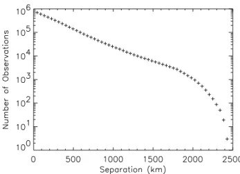
Fig. 1. The number of1vmeasurements as a function of separation lused in the calculation ofSfor the unconditioned data.
give 1v(l)=v(r+l, t )−v(r, t ). We then take the moduli of these values and average over all scans from the 8-year period (<|v(r+l, t )−v(r, t )|>). This is then repeated for all possible range gate separations from 1 (l=45 km) to 55 (l=2475 km) to give S1(l). Similar calculations are
per-formed for the second, third, fourth, fifth and sixth order structure functions (n=2,3,4,5, and 6 respectively). At the same time we calculate PDFs of the velocity differences1v
for each separationl, in bins of 10 m s−1.
3 Analysis of raw data
Figure 1 shows the occurrence frequency of 1v measure-ments as a function of separation l when the selection cri-teria described above are applied to the Halley SuperDARN data. There are many more data pairs at small separations than at larger ones. This is a result of two factors: (1) At any one time SuperDARN backscatter is only measured at a lim-ited (but variable) number of ranges. (2) The fact that we are considering only measurements made poleward of the OCB restricts the number of large separations. At a separation of 1 range gate (45 km) we have>105pairs of measurements. At 2000 km separation this falls to below 103data pairs.
Figure 2 shows the first three order structure functions plotted as a function of separation calculated using the al-gorithm presented above. It should be noted thatS2has been divided by 200 andS3has been divided by 50 000 in order
to show them clearly on the same figure asS1(it is the shape
Fig. 2. The first three order structure functions plotted as a function of separationlcalculated using unconditioned data (S1diamonds, S2squares,S3triangles). For convenienceS2has been divided by 200 andS3has been divided by 50 000. The red lines show straight lines fitted to the power-law region of each structure function.
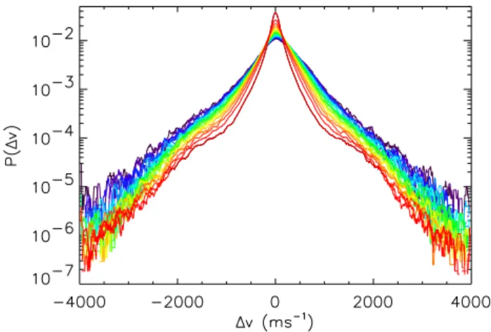
Fig. 3. PDFs of1vused in the calculation of structure functions for separations from 1 (red) to 20 (black) range cells (45–900 km). The data is plotted for 10 m s−1bins with a 9-point running mean applied.
The red lines in Fig. 2 show straight lines fitted to power-law regions of each line (using a least-squares fit to the points in log-log space, where the extent of the fit is selected by eye). The slope of the line in log-log space is the power-law exponentζn. The fitted power-law exponents are ζ1=0.31
(from 135 to 945 km), ζ2=0.48 (from 45 to 675 km) and ζ3=0.52 (from 90 to 585 km). In order to asses the sensi-tivity of our estimates ofζnto the fitting range we have also fitted the lines over half the number of data points. None of the fitted exponents presented in this paper change by more than 0.01.
In order to assess the validity of our calculated structure functions and their scaling exponents we study the PDFs
of the velocity fluctuations used in our calculations. These are shown in Fig. 3 for separations of 1 (red) to 20 (black) range cells (45–900 km). The data are plotted using 10 m s−1 bins with a 9-point running mean applied. The PDFs re-veal two possible sources of error. Firstly, statistical fluc-tuations increase with increasing 1v and increasing l due to a decreasing number of data samples. As the PDFs are non-Gaussian leptokurtic distributions the tails of the dis-tributions with larger statistical fluctuation error contribute significantly to the calculated structure functions (increas-ingly so for increasingn). Secondly, at around±2000 m s−1 there is a shoulder in the PDFs (most clearly seen in the red trace). This does not reflect the actual velocity fluctu-ations in the ionosphere but is due to the maximum velocity that can be measured by the radar. In common mode, Su-perDARN velocity measurements are aliased outside of the range |vmax|≈2000 m s−1 (which varies slightly depending
on the operational frequency of the radar). Hence, the maxi-mum velocity difference that can be measured is1v=2vmax.
Given that some measurements of1vwill have been calcu-lated whenv(r+l, t ) orv(r, t )(or both) have been aliased, the measured PDF of1vwill be different from the true PDF of the system. This effect will be most significant when1vis close to or greater thanvmaxand we believe this effect gives
rise to the shoulder seen in Fig. 3 at around±2000 m s−1. It should be remembered that only a small number of veloc-ity measurements will be aliased but due to the heavy tailed nature of the1v PDF it will have a significant effect when calculatingSn. The effect of aliasing on the PDF at small1v will be insignificant and the central core of the distribution is estimated well with low statistical fluctuation error.
The poor estimate of the PDF at large1vwill adversely affect the calculated structure functions shown in Fig. 2 and hence the scaling exponents found. The point at which this effect becomes significant is at a fixed velocity difference (≈vmax) and not at a fixed percentile of the distribution. To
tackle this problem and determine more accurate structure functions we need to remove the erroneous data at large1v
whilst retaining the same proportion of the distribution at each separationl.
4 Analysis of conditioned data
To correct for the sources of error described above we have applied a technique called conditioning. This removes data that is possibly erroneous by clipping the data used in the structure function calculations so that all fluctuations larger thanbσ1v(l)are ignored, wherebis a constant andσ1v(l) is the standard deviation of the velocity differences at range separation l. Applying the conditioning technique ensures that the same proportion of the parent distribution for eachl
modeled L´evy flight time series made calculations of struc-ture functions difficult because the moments are strongly in-fluenced by the tails of the distributions, which are poorly sampled statistically (i.e. rare). They demonstrated that by removing the poorly sampled data using conditioning, the known mono-fractal scaling behavior could be restored, i.e.ζn=nζ1. The same technique has also been applied to the
AE index (Chapman et al., 2005) and measurements of the solar wind (Hnat et al., 2003, 2005). Furthermore, a similar technique has been applied in wavelet spectral techniques in studies of atmospheric turbulence (i.e., Katul et al., 1994) and in the solar wind (Veltri and Mangeney et al., 1999; Bruno et al., 1999; Mangeney et al., 2001). Clearly using a condi-tioned data-set will not give a good absolute estimate ofSn. What we are really interested in is the scaling properties of
Sn(i.e.ζn), which may be based on part of the distributions. In their study, Chapman et al. (2005) clipped their data at b=5,10,15 and 20. However in our case we need to clip at a smallerbbecause we wish to remove not only the rarely sampled data but also the erroneous data that results from velocity aliasing. The effect of the aliasing is to intro-duce errors in the PDF at1v >∼2000 m s−1and thus we re-quirebσ1v<2000 m s−1. However, we do not need to satisfy this criteria for the whole data set as we are only concerned with a correct application of conditioning at the separations where scaling is seen (i.e. l<900 km). As σ1v increases withlthe largestbσ1vwe are concerned with occurs when l=900 km. At this separation σ1v=616 m s−1, and so we have chosen to clip our data atb=3 (i.e.bσ1v=1848 m s−1). In fact, clipping our data at 3σ1v ensures that fluctuations >±2000 m s−1are not used in the calculation ofSnfor sep-arations of 1035 km or less. By clipping atb=3 there is a 2% reduction in data overall compared to the unconditioned calculations. Proportionately most data is lost at small sepa-rations with a 2.1% reduction in data at 45 km separation and a 1.8% reduction in data at 900 km separation.
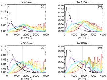
To understand better how the clipping affects the calcula-tion ofSn, and henceζn, and which order of structure func-tions we can trust, we investigate the partial distribution ofSn as a function of1v. Figure 4 presents histograms showing the proportion ofSnto come from each 100 m s−11vbin for n=1,2,3,4,5,6. Each panel in Fig. 4 shows the histograms for different separations from 45 km (a) to 900 km (d). The grey vertical lines in each panel show the 3σ1v clipping that has been applied i.e. we ignore all data to the right of the grey line.
In each panel of Fig. 4 we see that the peaks of the distri-butions are at small1vforS1, moving to increasing values
with increasing order. For the larger separations (panels c and d) the peak is hard to see for the higher order curves due to the statistical fluctuations. These fluctuations are due to poor sampling statistics and the emphasis of larger 1v for larger moments. It is clear that by clipping at 3σ1v we ig-nore most of these poorly sampled bins. More importantly,
Fig. 4. Partial distributions showing the proportion ofSnto come from each 100 m s−11vbin. Each panel shows the partial distri-bution for a different separation;(a)l=45 km,(b)l=315 km,(c) l=630 km and(d)l=900 km. Each panel shows the partial distri-butions for the first six order structure functions;n=1 (black),n=2 (purple),n=3 (blue),n=4 (green),n=5 (yellow), andn=6 (red).
if we look at the partial distribution ofS1(black line) we see
that for all separations the range of data included in our cal-culations (left of the grey line) includes most of the distribu-tion and certainly includes its peak and form. We would say that this is also true ofS2(purple line) especially when we
consider that the secondary peak seen in panel (a) between 1100 and 2000 m s−1is due to the aliasing problem that we are attempting to exclude. In the case ofS3it is much more marginal but we certainly would not trustS4,S5orS6, as our calculation only includes the lower tail of the partial distri-bution and hence we would not expect an accurate estimate ofζnfrom this.
Figure 5 shows the conditioned structure functions plotted as a function of separation for the first three orders. It should be noted thatS2 has been divided by 200 andS3 has been
divided by 50 000 as in Fig. 2. The same shape of line is seen in Fig. 5 as in Fig. 2 with power-law behavior seen at small separations and deviations due to the global convection cells seen at large separations. The red lines in Fig. 5 show straight lines fitted to power-law regions of each line (using a least-squares fit to the points in log-log space where the extent of the fit is selected by eye). The fitted power-law exponents areζ1=0.34 (from 135 to 945 km),ζ2=0.63 (from 45 to 675 km) andζ3=0.88 (from 90 to 585 km).
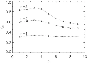
We have also tried conditioning at differentb between 1 and 9. The result of this different clipping is shown in Fig. 6. The clipping makes little difference to the value of ζ1
be-cause the tails of the1vPDF make little contribution toS1.
Fig. 5. The first three order structure functions plotted as a function of separationlcalculated using conditioned data (S1diamonds,S2 squares,S3triangles). For convenienceS2has been divided by 200 andS3has been divided by 50 000. The red lines show straight lines fitted to the power-law region of each structure function.
Fig. 6. The variation of the fitted power-law exponentsζnfor differ-ent levels of clippingbfor the first three order structure functions.
the arguments above). Whenb≤3, reasonably similar results give us confidence in the robustness of the results presented above (Fig. 5). There is some small variation forb≤3 which will occur due to sampling less of the core of the partial dis-tributions shown in Fig. 4.
5 P (0)scaling
In addition to the structure functions shown above, further information can be gleaned about the structure of the iono-spheric plasma velocities by calculating the peak, orP (0), scaling. Figure 7 shows the peak values of the PDFs of ionospheric velocity fluctuations as a function of separa-tion. Here we see a power law region from∼135 km to over
Fig. 7. Peaks of the PDFs of 1v as a function of separationl (diamonds). The red line shows a straight line fitted to the power-law region of theP (0)line.
1000 km. The red line in Fig. 7 shows a straight line fitted over the range 135–945 km (again using a least-squares fit to the line in log-log space where the extent of the fit is se-lected by eye). The fitted power-law exponent is−0.40. It is worth noting that theP (0)scaling is not affected by the same issues that made calculating the structure functions dif-ficult. The peaks of our PDFs always occur close to zero and so they are not significantly affected by the aliasing problem discussed above. Moreover, they are calculated from the re-gion with the best statistics, i.e. the part of the distribution we capture best.
6 Discussion
6.1 Comparison with turbulence models
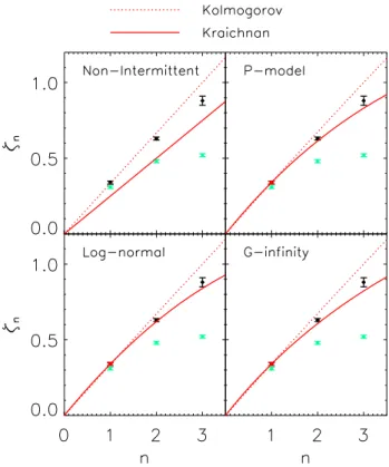
Figure 8 showsζn as a function of nfor the first three or-der structure functions (black and red points), and compares these measured values against eight different models of tur-bulence (red lines). The models shown are the “classic” (non-intermittent) Kolmogorov (K41) and Kraichnan-Iroshnikov (KI65) models along with Kolmogorov and Kraichnan ver-sions of the intermittentP, log-normal, and G-infinity mod-els. The equations used to determine these model lines are given in the appendix along with the values of any free pa-rameters used. The non-intermittent K41 and KI65 models have no free parameters. All other models have one free pa-rameter which has been determined using ζ1, the best
Fig. 8. S1,S2andS3calculated from the conditioned plasma ve-locity data (black and red points) compared to eight different turbu-lence models. In each panel Kolmogorov (dotted line) and Kraich-nan (solid line) versions are plotted. Details of theζnvs.n relation-ships can be found in the appendix along with the values of the free parameters used. The points plotted in red have been used to derive free parameters and so will give perfect agreement with the plotted curves. Points plotted in black do not constrain the plotted curves in any way. Also shown are the values ofS1,S2andS3calculated from the unconditioned plasma velocity data (green points).
selection of the region of fit (∼0.1) and the error on the least squares fit (∼0.003) neither of which will affect the error bars shown in Fig. 8.
At the most conservative level we consider that onlyζ1is wholly trustworthy. In this case, we cannot judge the good-ness of fit of the intermittent models as the free parameters have been determined usingζ1. However, it is interesting to note that all of the Kolmogorov-type intermittent models are very close to the non-intermittent version. This is be-causeζ1is very close to the value of 1/3 predicted for K41.
Conversely the non-intermittent KI65 does not agree withζ1
and the fitted Kraichnan-type models all show significant in-termittency. Let us now take a more liberal view of what moments we can trust and considerζ1 andζ2 and possibly ζ3. The Kolmogorov-type models all give good agreement
withζ1andζ2but notζ3. The intermittent Kraichnan models
give good agreement withζ2(andζ1by construction) and a
reasonable agreement withζ3considering the uncertainty of
this value. The Kraichnan versions of the log-normal model
gives the best agreement with our data followed by the P model and then the G-infinity model. It should be noted that all Kolmogorov-based models are constrained such that
ζ3=1 which does not agree with our measuredζ3value.
One might argue that it is not fair to compareζ values calculated from our conditioned data to the analytical pre-dicted values for different turbulence models in the absence of conditioning. By removing large fluctuations from our cal-culations we are removing some of the intermittency which gives rise to theζ vsnrelationships predicted for intermittent models of turbulence (such as theP-models shown here) and thus we might expect differentζ vsnrelationships for condi-tioned data. It is for precisely this reason that we have chosen to ignoreζnwhenn≥4. Forζ1we argue that the amount of the partial distribution ofS1that is included in our calcula-tions is enough that we represent the true value ofζ1well, or conversely that the expected value ofζ1 from a model will not change significantly when the model is subjected to con-ditioning. As we have explained above, the argument is less strong forζ2and marginal forζ3.
Based on structure functions alone, and knowing thatζ3is
questionable, it is hard to argue that any one model shown in Fig. 8 better agrees with our data than any other (except for dismissing the non-intermittent KI65). However, we can use the fact that we know P (0)has a scaling exponent of 0.40 to add more information. As we mentioned above the fitted Kolmogorov-type models were all close to the non-intermittent version. The non-intermittent K41 model is a mono-fractal, i.e. it has only one scaling exponent and
ζn=nζ1. If our data were described by a mono-fractal we would expectP (0)to scale with the same exponentζ1. The reason for this is trivial when considering Guassian fluctua-tions with zero mean whereP (0)=1/√2π σand the standard deviation,σ, is equal to√S2 and scales with the exponent ζ2/2=ζ1. More generally ifvwere self affine then
P (1v, l)=l−ζ1φ
1v
lζ1
(3) (e.g., Krishnamurthy et al., 2000) henceP (1v=0, l)scales asl−ζ1.
The factP (0)scales differently toζ1indicates that the
sys-tem is a multi-fractal and therefore supports an intermittent model over a non-intermittent one. Based on this extra infor-mation we suggest that the Kraichnan versions of the P and log-normal models give better agreement with our data than K41.
6.2 The validity of conditioning
by conditioning data taken from an intermittent turbulent medium (e.g. atmospheric turbulence, Katul et al., 1994, and solar wind turbulence, Mangeney et al., 2001), the mono-fractal component is extracted and any signature of multi-fractality is lost. Moreover, this mono-fractal component re-lates directly to non-intermittent turbulence models, such as K41, in the inertial range. In this section we discuss how our data may be interpreted given these concerns.
Firstly, we consider how one might interpret our data if we did not employ conditioning. The rationale for doing this would be along the lines that, although the aliasing effect of the radar does remove some large fluctuations from our data set and include some spurious ones, it still includes all of the large fluctuations measured and so would give the best estimate of the intermittent nature of the data. For compari-son the values ofζnfor the unconditioned data are shown in Fig. 8 as green points. The error bars of±0.01 are estimated from the variation in ζn when fitting over different ranges of1v. The unconditionedζn do indeed show strong inter-mittent behavior, as indicated by the deviation from a linear relationship in Fig. 8. However, it is very hard to interpret these data in terms of current turbulence models. All inter-mittent models of turbulence we have tested against in this paper (along with any others we are aware of) are constrained in two ways. 1)ζ3=1 for Kolmogorov type turbulence (a di-rect consequence of the four-fifths law (e.g., Frisch, 1995, pp 76 and 133)) andζ4=1 in the Kraichnan formalism, and 2) ζn>n/3 forn<3 in the Kolmogorov cases (e.g., Frisch, 1995, pp 133) andζn>n/4 forn<4 in the Kraichnan cases. As can be seen in Fig. 8, our unconditionedζn do not meet these constraints. If one was to consider the unconditioned data as the best estimate of intermittency then it can not be described by current turbulence models and a different physi-cally motivated multi-fractal model and/or theory would have to be found. It is interesting to note that the unconditioned structure functions calculated by Mangeney et al. (2001) us-ing solar wind data do not meet these conditions either.
Secondly, we consider the implications if one considers that strong conditioning, such as we have employed here, ex-tracts the mono-fractal turbulent component. In Sect. 4 we argued that ourζn values forn>3 could not be trusted and ζ3was questionable. However, these arguments were made based on our ability to measure intermittency. If we now consider that our conditioning does extract the mono-fractal component, and that we can ignore intermittency altogether, there is no longer any reason to doubt the validity ofζ3 or
indeed any higherζnvalues. Looking at the conditioned data in Fig. 8 we see thatζ1andζ2are consistent with the
non-intermittent Kolmogorov model butζ3is not. Theζnin Fig. 8 are close to having a linear relationship withnas might be expected for a mono-fractal but such a line would not pass through the origin by definition. We conclude from this that strong conditioning does not extract purely the mono-fractal component. Furthermore, if we consider other values ofζn conditioned at 3σ1v (ζ4=1.09, ζ5=1.33, ζ6=1.57)the case
for a mono-fractal is harder to make.
The final thing we consider is the possibility that by con-ditioning our data we are removing contributions to inter-mittency from large fluctuations and that ourζn values are less intermittent than the real turbulent reality. This is almost certainly true, but what really matters is how significant is the error introduced is. In Sect. 4 we showed using Fig. 4 that the main contribution toζ1 came from small values of
1v(generally<1.5σ1v) and that the main contribution toζ2 came from slightly larger values of1v (generally between 0.5 and 2.5σ1v). There may be contributions toζ1 andζ2 coming from higher values of1v which were ignored due to the aliasing effect or conditioning (or both) but given the amount of data lost due to conditioning (∼2%) these contri-butions would have to occur at a very large1vindeed to be significant.
If we look at the three curves shown in Fig. 6 we see that forζ1,ζ2 andζ3there is a peak in their value when
condi-tioning at 3σ1v. When we consider the constraints outlined above for intermittent turbulence models we find that condi-tioning at 3σ1vresults in the most intermittent estimates of ζnconsistent with turbulence theory.
7 Summary and conclusions
In this paper we have presented a detailed structure function analysis of the ionospheric plasma velocity in the nightside ionosphere, poleward of the OCB, as measured by the Halley SuperDARN radar. We have found that the maximum veloc-ity that can be measured by the SuperDARN radars restricts our ability to accurately calculate structure functions. How-ever, we correct for this effect by conditioning our data be-fore calculating the structure functions such that fluctuations
>3σ1vare removed. By studying the partial distributions of the structure functions as a function of1v, we suggest that structure functions of order 3 and less may be used. The scal-ing exponents found as a result of this, along with the P(0) scaling exponent, suggest that the Kraichnan versions of ei-ther the P or log-normal model of turbulence best describes the velocity structure seen in the ionosphere, but to distin-guish between these would require accurate determinations ofζnforn>3.
changes in coupled environments with different symmetries in the equations which describe these environments.
Addendum
During the reviewing process of this paper certain concerns were raised questioning the validity of the analysis presented here. These concerns relate to the conditioning technique that we have employed. It was suggested that this technique, by removing the largest fluctuations, reduces the intermit-tency that is measured. As a consequence, it was suggested that the unconditioned data provides a better estimate of the intermittency in the ionospheric velocity fluctuations than the conditioned data. Our view is that this is not the case and that the best estimate of the intermittency for this data set is pro-vided by the conditioned data for the reasons presented in the paper.
Appendix A Turbulence models
Below are the equations forζn for the different models of turbulence shown in Fig. 8 along with the values used for any parameters. See Pagel and Balogh (2001) and references therein for further details. The G-infinity model is an in-termittency model rather than a turbulence model but can be adapted for turbulence by introducing the Kolmogorov or Kraichnan constraint thatζ3=1 orζ4=1, respectively.
Sim-ilarly, we have adapted the parameters in the log-normal model to meet the constraintζ4=1 in the Kraichnan version.
K41
ζn=n/3 (A1)
KI65
ζn=n/4 (A2)
P model of K41
ζn=1−log2
pn/3+(1−p)n/3 (A3)
wherep=0.601. P model of KI65
ζn=1−log2
pn/4+(1−p)n/4 (A4)
wherep=0.854.
Lognormal – Kolmogorov version
ζn= n
3+
µ
18(3n−n
2)
(A5) whereµ=0.03
Lognormal – Kraichnan version
ζn= n
4+x(4n−n
2)
(A6)
wherex=0.03
G-infinity – Kolmogorov version
ζn=
g(∞)n
3g(∞)−3+n (A7)
Whereg(∞)=34.0.
G-infinity – Kraichnan version
ζn=
g(∞)n
4g(∞)−4+n (A8)
Whereg(∞)=2.83.
Acknowledgements. We would like to thank G. King, S. Chapman, K. Kiyani and R. Woodard for useful discussions.
Edited by: T. Chang
Reviewed by: three anonymous referees
References
Abel, G. A., and Freeman, M. P.: A statistical analysis of iono-spheric velocity and magnetic field power spectra at the time of pulsed ionospheric flows, J. Geophys. Res., 107, 1470, doi:10.1029/2002JA009402, 2002.
Abel, G. A., Freeman, M. P., and G. Chisham: Spatial struc-ture of ionospheric convection velocities in regions of open and closed magnetic field topology, Geophys. Res. Lett., 33, L24103, doi:10.1029/2006GL027919, 2006.
Bering, E. A., III, Benbrook, J. R., Byrne, G. J., Liao, B., Theal, J. R., Lanzerotti, L. J., and Maclennan, C. G.: Balloon measure-ments above the South Pole: Study of ionospheric transmission of ULF waves, J. Geophys. Res., 100, 7807–7819, 1995. Bohr, T., Jensen, M. H., Paladin, G., and Vulpiani, A.:
Dynami-cal systems approach to turbulence, Cambridge University Press, UK, 1998.
Borovsky, J. E., Elphic, R. C., Funsten, H. O., and Thomsen, M. F.: The Earth’s plasma sheet as a laboratory for flow turbulence in high-βMHD, J. Plasma Phys., 57, 1–34, 1997.
Bruno, R., Bavassano, B., Pietropaolo, E., Carbone, V., and Vel-tri, P.: Effects of intermittency on interplanetary velocity and magnetic field fluctuations anisotropy, Geophys. Res. Lett., 26, 3185–3188, 1999.
Buchert, S. C., Fujii, R., and Glassmeier, K.-H.: Ionospheric con-ductivity modulation in ULF pulsations, J. Geophys. Res., 104, 10 119–10 133, 1999.
Campbell, W. H.: An analysis of the spectra of geomagnetic varia-tions having periods from 5 min to 4 hours, J. Geophys. Res., 81, 1369–1390, 1976.
Chang, T.: Low-dimensional behavior and symmetry-breaking of stochastic systems near criticalityCan these effects be observed in space and in the laboratory, IEEE Trans. Plasma Sci., 20, 691– 694, 1992.
Chisham, G. and Freeman, M. P.: A technique for accurately deter-mining the cusp-region polar cap boundary using SuperDARN HF radar measurements, Ann. Geophys., 21, 983–996, 2003, http://www.ann-geophys.net/21/983/2003/.
Chisham, G. and Freeman, M. P.: An investigation of latitudinal transitions in the SuperDARN Doppler spectral width parameter at different magnetic local times, Ann. Geophys., 22, 1187–1202, 2004,
http://www.ann-geophys.net/22/1187/2004/.
Chisham, G., Freeman, M. P., and Sotirelis, T.: A statistical comison of SuperDARN spectral width boundaries and DMSP par-ticle precipitation boundaries in the nightside ionosphere, Geo-phys. Res. Lett., 31, L02804, doi:10.1029/2003GL019074, 2004. Chisham, G., Freeman, M. P., Sotirelis, T., Greenwald, R. A., Lester, M., and Villain, J.-P.: A statistical comparison of Su-perDARN spectral width boundaries and DMSP particle precip-itation boundaries in the morning sector ionosphere, Ann. Geo-phys., 23, 733–743, 2005,
http://www.ann-geophys.net/23/733/2005/.
Chisham, G., Lester, M., Milan, S. E., Freeman, M. P., Bristow, W. A., Grocott, A., McWilliams, K. A., Ruohoniemi, J. M., Yeoman, T. K., Dyson, P. L., Greenwald, R. A., Kikuchi, T., Pinnock, M., Rash, J. P. S., Sato, N., Sofko, G. J., Villain, J.-P., and Walker, A. D. M.: A decade of the Super Dual Auro-ral Radar Network (SuperDARN): Scientific achievements, new techniques and future directions, Surv. Geophys., 28, 33–109, doi:10.1007/s10712-007-9017-8 2007.
Consolini, G., De Michelis, P., Meloni, A., Cafarella, L., and Can-didi, M.: L´evy-stable probability distribution of magnetic field fluctuations at Terra Nova Bay (Antarctica), Proc. Italian Res. On Antarctic Atmosphere, 367–376, Soc. Ital. di Fisica, Bologna, Italy, 1998.
Francia, P., Villante, U., and Meloni, A.: An analysis of geomag-netic field variations (3 min–2 h) at a low latitude observatory (L=1.6), Ann. Geophys., 13, 522–531, 1995,
http://www.ann-geophys.net/13/522/1995/.
Freeman, M. P., Watkins, N. W., and Riley, D. J.: Evidence for a solar wind origin of the power law burst lifetime distribution of the AE indices, Geophys. Res. Lett., 27, 1087–1090, 2000. Frisch, U.: Turbulence, Cambridge University Press, Cambridge
U.K., 1995.
Greenwald, R. A., Baker, K. B., Dudeney, J. R., Pinnock, M., Jones, T. B., Thomas, E. C., Villain, J.-P., Cerisier, J.-C., Senior, C., Hanuise, C., Hunsucker, R. D., Sofko, G., Koehler, J., Nielsen, E., Pellinen, R., Walker, A. D. M., Sato, N., and Yamagishi, H.: DARN/SuperDARN: A global view of the dynamics of high-latitude convection, Space Sci. Rev., 71, 761–796, 1995. Grossman, S., Lohse, D., and Reeh, A.: Application of extended
self-similarity in turbulence, Phys. Rev. E, 56, 5473–5478, 1997. Golovchanskaya, I. V., Ostapenko, A. A., and Kozelov, B. V.: Re-lationship between the high-latitude electric and magnetic turbu-lence and the Birkeland field-aligned currents, J. Geophys. Res., 111, A12301, doi:10.1029/2006JA011835, 2006.
Hnat, B., Chapman, S. C., Rowlands, G., Watkins, N. W., and Freeman, M. P.: Scaling of solar wind and the AU, AL and AE indices as seen by WIND, Geophys. Res. Lett., 29, 2078, doi:10.1029/2002GL016054, 2002.
Hnat, B., Chapman, S. C., Rowlands, G., Watkins, N. W., and Free-man, M. P.: Scaling in long term data sets of geomagnetic
in-dices and solar windǫas seen by WIND spacecraft, Geophys. Res. Lett., 30, 2174, doi:10.1029/2003GL018209, 2003. Hnat, B., Chapman, S. C., and Rowlands, G.: Scaling and a
Fokker-Planck model for fluctuations in geomagnetic indices and com-parison with solar windǫas seen by Wind and ACE, J. Geophys. Res., 110, A08206, doi:10.1029/2004JA010824, 2005.
Kamide, Y. and Baumjohann, W.: Magnetospher-ionosphere cou-pling, Springer-Verlag, Berlin Heidelberg, 1993.
Katul, G. G., Parlange, M. B., and Chu, C. R.: Intermittency, lo-cal isotropy, and non-Gaussian statistics in atmospheric surface-layer turbulence, Phys. Fluids, 6, 2480–2492, 1994.
Kintner, P. M.: Observations of velocity shear driven plasma turbu-lence, J. Geophys. Res., 81, 5114–5122, 1976.
Kozelov, B. V., Uritsky, V. M., and Klimas, A. J.: Power law probability distributions of multiscale auroral dynamics from ground-based TV observations, Geophys. Res. Lett., 31, L20804, doi:10.1029/2004GL020962, 2004.
Krishnamurthy, S., Tanguy, A., Abry, P., and Roux, S.: A stocastic description of external dynamics, Europhys. Lett., 51, 1–7, 2000. Lui, A. T. Y., Chapman, S. C., Liou, K., Newell, P. T., Meng, C. I., Brittnacher, M., and Parks, G. K.: Is the dynamic magnetosphere an avalanching system?, Geophys. Res. Lett., 27, 911–914, 2000. Mangeney, A., Salem, C., Veltri, P. L., and Cecconi, B.: Intermit-tency in the solar wind turbulence and the Haar wavelet trans-form, in: Sheffield space plasma meeting: multipoint measure-ment versus theory, Proc. - Les Woolliscroft memorial confer-ence, 53–64, 2001.
Pagel, C., and Balogh, A.: A study of magnetic fluctuations and their anomalous scaling in the solar wind: the Ulysses fast-latitude scan, Nonlinear Prog. Geophys., 8, 313–330, 2001. Parkinson, M. L.: Dynamical critical scaling of electric field
fluc-tuations in the greater cusp and magnetotail implied by HF radar observations of F-region Doppler velocity, Ann. Geophys., 24, 689–705, 2006,
http://www.ann-geophys.net/24/689/2006/.
Pulkkinen, A., Klimas, A., Vassiliadis, D., Uritsky, V., and Tan-skanen, E.: Spatiotemporal scaling properties of the ground geomagnetic field variations, J. Geophys. Res., 111, A03305, doi:10.1029/2005JA011294, 2006.
Ruohoniemi, J. M. and Greenwald, R. A.: Dependencies of high-latitude plasma convection: Consideration of inter-planetary magnetic field, seasonal, and universal time fac-tors in statistical patterns, J. Geophys. Res., 110, A09204, doi:10.1029/2004JA010815, 2005.
Ruohoniemi, J. M., Greenwald, R. A., Baker, K. B., and Villain, J.-P.: Drift motions of small-scale irregularities in the high lat-itude F region: An experimental comparison with plasma drift motions, J. Geophys. Res., 92, 4553–4564, 1987.
Takalo, J., Timonen, J., and Koskinen, H.: Correlation dimension and affinity of AE data and bicolored noise, Geophys. Res. Lett., 25, 1527–1530, 1993.
Takalo, J. and Timonen, J.: Comparison of the dynamics of the AU and PC indices, Geophys. Res. Lett., 25, 2101–2104, 1998. Taylor, G. I.: The spectrum of turbulence, Proc. R. Soc. London,
Ser. A, 164, 476–490, 1938.
doi:10.1029/2001JA000281, 2002.
Veltri, P. and Mangeney, A.: Scaling laws and intermittent struc-tures in solar wind MHD turbulence, in: Solar Wind 9, AIP Con-ference Proceedings, 471, 543–546, 1999.
Villain, J.-P., Caudal, G., and Hanuise, C.: A SAFARI-EISCAT comparison between the velocity of F region small-scale irregu-larities and the ion drift, J. Geophys. Res., 90, 8433–8443, 1985.
Weatherwax, A. T., Rosenberg, J. T., Lanzerotti, L. J., Maclennan, C. G., Frey, H. U., and Mende, S. B.: The distention of the mag-netosphere on 11 May 1999: High latitude Antarctic observa-tions and comparisons with low latitude magnetic and geopoten-tial data, Geophys. Res. Lett., 27, 4029–4032, 2000.