Ensaios Econômicos
Escola de
Pós-Graduação
em Economia
da Fundação
Getulio Vargas
N◦ 727 ISSN 0104-8910
The effect of social security, health,
demog-raphy and technology on retirement
Ferreira, Pedro Cavalcanti, Santos, Marcelo Rodrigues dos
Os artigos publicados são de inteira responsabilidade de seus autores. As
opiniões neles emitidas não exprimem, necessariamente, o ponto de vista da
Fundação Getulio Vargas.
ESCOLA DE PÓS-GRADUAÇÃO EM ECONOMIA Diretor Geral: Rubens Penha Cysne
Vice-Diretor: Aloisio Araujo
Diretor de Ensino: Carlos Eugênio da Costa
Diretor de Pesquisa: Luis Henrique Bertolino Braido Direção de Controle e Planejamento: Humberto Moreira Vice-Diretor de Graduação: André Arruda Villela
Pedro Cavalcanti, Ferreira,
The effect of social security, health, demography and technology on retirement/ Ferreira, Pedro Cavalcanti, Santos, Marcelo Rodrigues dos – Rio de Janeiro : FGV,EPGE, 2012
43p. - (Ensaios Econômicos; 727)
Inclui bibliografia.
The E¤ect of Social Security, Health, Demography and
Technology on Retirement
Pedro Cavalcanti Ferreira
yand Marcelo Rodrigues dos Santos
zAbstract
This article studies the determinants of the labor force participation of the elderly and investigates the factors that may account for the increase in retirement in the second half of the last century. We develop a life-cycle general equilibrium model with endogenous retirement that embeds Social Security legislation and Medicare. In-dividuals are ex ante heterogeneous with respect to their preferences for leisure and face uncertainty about labor productivity, health status and out-of-pocket medical ex-penses. The model is calibrated to the U.S. economy in 2000 and is able to reproduce very closely the retirement behavior of the American population. It reproduces the peaks in the distribution of Social Security applications at ages 62 and 65 and the ob-served facts that low earners and unhealthy individuals retire earlier. It also matches very closely the increase in retirement from 1950 to 2000. Changes in Social Security policy - which became much more generous - and the introduction of Medicare account for most of the expansion of retirement. In contrast, the isolated impact of the increase in longevity was a delaying of retirement.
Key words: Retirement; Social Security; Health Shocks; Medicare; Aging Popu-lation.
JEL classi…cation: J2; E2; D5
We wish to thank Flávio Cunha, Rodrigo Soares, Carlos Eugênio da Costa, Samuel Pessôa, Ricardo Cavalcanti, Luiz Braido and Cesar Santos as well as seminar participants at EPGE-FGV, USP, IBMEC-RJ, Insper, at the 2011 SED meeting in Ghent, at the 2011 EEA annual Congress in Oslo and at the 2008 SBE meetings in Bahia for helpful comments. We are responsible for any remaining errors. The authors acknowledge the …nancial support of CAPES and CNPQ.
yGraduate School of Economics ( EPGE ), Fundação Getulio Vargas, Praia de Botafogo 190, 1125, Rio
de Janeiro, RJ, 22253-900, Brazil. Email: [email protected].
1
Introduction
The reduction of the participation of elderly people in the labor force was one of most remarkable economic changes of the last century, particularly in the second half. In 1950, 46% of men aged 65 and over in the United States were working, but only 16.5% were in 2000. Just four out of every ten 66-year-old males were retired in 1950, but …fty years later almost seven out of ten were out of the labor force. This phenomenon is hardly exclusive to the United States. Blondal and Scarpetta (1998) and Gruber and Wise (1999) provide evidence that the workforce participation of the elderly population has declined in many countries of the OECD.
Currently, more than 50% of workers choose to retire at the age of 62, when they …rst become eligible for early retirement bene…ts under social security, although at a reduced level. In 1950, in contrast, there was no legal early retirement age and the minimum and normal retirement age coincided at 65. The decision to retire, and to do it early, is in‡uenced by a number of factors in addition to age and the rules of social security such as health status, income, preference for leisure, etc. For instance, according to data from the Health and Retirement Survey, approximately 90% of individuals between 55 and 85 years of age who declared themselves in poor health were retired in 2000, compared with only 40% of those in excellent health.
This article develops and calibrates a lifeclycle general equilibrium model with heteroge-neous agents to study the determinants of the labor force participation of elderly American males and to investigate the factors that may account for the changes in retirement between 1950 and 2000. We focus on the role of Social Security, health status and the introduc-tion of Medicare, demographic factors (associated with higher longevity) and changes in the age-e¢ciency pro…le.
idiosyncratic shocks.
In addition, we model the U.S. Social Security system in detail and also allow agents to decide when to start collecting retirement bene…ts regardless of their employment status. This is consistent with the empirical evidence in Rust and Phelan (1997) and Benítez-Silva and Heiland (2008), who show that a large number of agents claim bene…ts while continuing to work, mainly among the nearly elderly ones.
We also take into account Medicare, which was introduced in 1965 and constitutes a fed-eral health insurance program that provides subsidized health insurance coverage to virtually every American over age 65. Medicare provides generous insurance against medical expendi-tures shocks and could induce earlier retirement because of the limited need to accumulate precautionary savings. Conversely, because of eligibility requirements, it also encourages the delay of retirement until 65.
The model is calibrated to the U.S. economy in 2000, our benchmark year, and is able to reproduce very closely the retirement behavior of the American population. In particular, the model reproduces the peaks in the distribution of Social Security applications at ages 62 and 65 and the observation that unhealthy and poor individuals retire earlier.
The model is then simulated considering the changes in Social Security, Medicare, age-e¢ciency pro…le and demography between 1950 and 2000. We …nd that the simulated labor force participation of older individuals increases to levels similar to those in the data. We show that the incentives implied by the institutional factors concerning Social Security and Medicare legislation are very e¤ective in in‡uencing retirement behavior. For instance, a counterfactual experiment in which all parameters were kept at their 2000 values, but the rules of Social Security were changed to those of 1950, …nds that the retirement rate drops for every age group. More importantly, the retirement peak at age 62 disappears, as in 1950 when there was no early retirement bene…ts.
Conde-Ruiz and Galasso (2003) endogenize retirement, but in a purely theoretical political-economy framework with no quantitative analysis. French (2005, 2011) estimates a partial equilibrium lifecycle model of retirement behavior in which health and wages are uncertain. He uses the model to simulate the impact on the labor supply of modi…cations to Social Se-curity legislation. Diaz-Gimenez and Diaz-Savavedra (2009) use an overlapping generational model with an endogenous retirement decision to study pension system reform in Spain. Our model has many features in common with theirs; but as we study the American economy, the calibration and institutional details of the model are obviously very di¤erent as are the experiments we run. Finally, in Kopecky (2011) whereas the decision to leave the labor force is endogenous as in our article, hours worked are …xed in every period and there is no social security in the model, which plays an important role in our case.1
As for the channels we emphasize as a¤ecting retirement behavior, the importance of higher Social Security bene…ts has been investigated in a number of articles using a variety of estimation methods.2 Nevertheless, this literature has not come to a consensus. In fact,
whereas Gustman and Steimeier (1986) and Rust and Phelan (1997) have found that Social Security bene…ts have had a strong negative e¤ect on male labor supply, Burtless (1986), Stock and Wise (1990) and Krueger and Pischke (1992) concluded that it had little e¤ect. These results suggest that either there are problems associated with the methods that have been used to investigate this relationship,3 or there are other explanations that must be
taken into consideration.4 In this article, we bring together, in a single model, di¤erent
explanations for the decision to retire.
The impact of health status and Medicare on retirement has also been investigated by Rust and Phelan (1997) and French and Jones (2005, 2011). However, they do not study the evolution of retirement over the last decades, which is a major goal of this paper. Ad-ditionally, none of these articles include home production, which is an important factor for the model to be able to reproduce the pattern of consumption over the lifecycle (Aguiar and
1Another related reference is Eisensee (2005) who uses a similar method to study how changes in the
Social Security system in the U.S. a¤ected retirement. His model, however, does not allow for idiosyncratic shocks - an important feature of our model - or health status, which we found to be important in the decision to leave the labor force.
2A recent survey of the literature can be found in Coile and Gruber (2007).
3Coile and Gruber (2007), for example, argue that some of these studies consider social security impacts
at a point in time, but not the e¤ects that arise from the time pattern of social security wealth accruals.
4Krueger and Pischke (1992) raise this point, after …nding little e¤ect of social security bene…ts on labor
Hurst, 2005).5
Regarding the impact of the rise in longevity on the decision to leave the labor force, Kalemli-Ozcan and Weil (2010) show that an exogenous decrease in the probability of death, which allows people to better plan saving for old age, generates a longer retirement life. In contrast, Bloom et al. (2007) show that, depending on social security provisions, improve-ments in life expectancy may induce people to remain in the labor force to increase savings for old age. Our simulations show that the latter e¤ect dominates.
Finally, technology change may modify age-earnings pro…les and hence the decision to leave the labor force, as shown by Ferreira and Pessôa (2007)6. In fact, Heckman, Lochner
and Todd (2003) provide evidence that older workers have become less productive relative to younger workers over the second part of the last century. This trend could induce people to work more intensively in the …rst part of their productive life, increase savings and retire earlier7.
The article is organized as follows. Some retirement facts are presented in Section 2. The model is presented in Section 3 and the calibration procedures and data are presented in Section 4. In Section 5 results are presented and discussed; Section 6 concludes.
2
Retirement Facts
This section presents the main facts that serve as outputs in our analysis. In particular, we document the changes in retirement between 1950 and 2000, the pattern of labor force participation by health status and by labor productivity, the distribution of applications for Social Security bene…ts, as well as the pattern of consumption over the life-cycle.
Panel A in Figure 1 presents the retirement pro…le by age for the years 1950 and 2000, which were constructed using data from the Integrated Public Use Microdata Series (IPUMS) for men aged 50 and over. The retirement rate is the ratio of the number of men who are retired to the number of men either in the labor force or retired. To be classi…ed as retired a
5In addition, aside from being partial equilibrium models, in Rust and Phelan (2007) individuals are
not allowed to save and, due to data restrictions, French and Jones (2005, 2011) consider a much shorter life-cycle.
6Note, however, that Ferreira and Pessôa (2007) use a representative agent economy and do not include
social security in their model.
7Graebner (1980) argues that in periods of rapid technological innovation, such as the last thirty years,
man must be completely out of the labor force. Thus, men who are working time or part-year are counted as working and not retired. The retirement rates for each age are computed by observing that: %retired = (% not in the labor force % never participating)=(1 %
never participating):8
The …gure displays the increase in retirement observed in the second half of the last century. It can be seen that the share of individuals out of the labor force is signi…cantly larger in 2000 than in 1950, mainly among those aged 60 and over. In 2000, there were very few people still working at age 75 - less than 10% - but in 1950 approximately 25% of the individuals of that age were still in the labor market. The main goal of this paper is to understand the causes of the changes presented in Panel A of Figure 1.
50 55 60 65 70 75 80 85 90 95
0 10 20 30 40 50 60 70 80 90 100
A) Individuals Out of the Labor Force (%)
Age
2000 1950
62 63 64 65 66 67 68 69 70
0 5 10 15 20 25 30 35 40 45 50 55
B) Distribution of Applications for SS Benefits (%)
Age
2000
Figure 1: Individuals out of the labor force (IPUMS, 1950 and 2000), distribution of Social Security bene…t claims (SSA, 2002).
Panel B in Figure 1, which shows the distribution of Social Security bene…t claims, suggest that institutional factors are very important in in‡uencing retirement behavior. The minimum age for eligibility for Social Security bene…ts in 2000 was 62, whereas the normal age for retirement bene…ts (without discount) was 65. The latter is also the age at which eligibility for Medicare starts. There are two peaks in the distribution of applications to
8This calculation is similar to that used in Kopecky (2011). Following Rust and Phelan (1997) we
social security bene…ts at these ages in 2000, as shown in Figure 2. Fifty-two percent of all applications occur at age 62, and 18% occur at age 65, twice as large as the number of applications at age 64. In 1950, however, the most common retirement age was 65.9
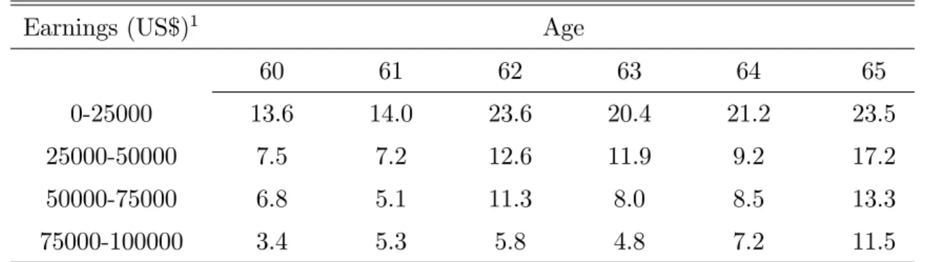
Table 1, which was constructed using U.S. Census data from 2000, presents evidence that low earners retire earlier. In the …rst column, we show earnings for individuals who worked at least 35 hours per week in the previous 12 months, whereas in the other columns we show the share of agents out of the labor force for di¤erent ages in 2000. It can be seen that labor force participation increases with earnings. In particular, more than 23% of individuals aged 65 with earnings up to $25000 in the previous year had already left the labor force in 2000, which is nearly twice as much as the share of agents with the same age and with earnings from $75000 to $100000.10
Table 1: Individuals Out of the Labor Force by Past Earnings (%) - 2000 Earnings (US$)1 Age
60 61 62 63 64 65
0-25000 13.6 14.0 23.6 20.4 21.2 23.5 25000-50000 7.5 7.2 12.6 11.9 9.2 17.2 50000-75000 6.8 5.1 11.3 8.0 8.5 13.3 75000-100000 3.4 5.3 5.8 4.8 7.2 11.5
1Received by individuals in the past 12 months who worked at least 35 hours per week.
Further evidence on the e¤ect of earnings on retirement can be found in Burkhauser, Couch and Phillips (1996). These authors use data from the Health and Retirement Survey (HRS) to compare those who take Social Security retirement bene…ts at age 62 with those who do not. They found that those who retired at the minimum age had a median income in 1993 of $31000 and those who postponed retirement had a median income of $41000. They found similar results when using the 1991 survey.
Although in the present article we do not deal with education, data on retirement by schooling level can be used as an indirect evidence of retirement by income level, given the strong positive correlation between income and education. In 2000, 57.4% of male
9Data on the distribution of Social Security bene…t claims is from the SSA’s Annual Statistical
Supple-ment, 2002
10According to the Census questionnaire, labor force status is determined by asking individuals whether
individuals aged 55-64 years with less than a high education were out of the labor force, but only 27% of those with a college degree or more were retired. For those aged 65-74 years, the corresponding …gures were 87.5% and 69%, respectively.
Studies of health status and retirement tend to indicate that those in poor health retire earlier, although there are complications in this case related to the fact that health status is not directly observable. For instance, McGarry (2004) found that poor health has a large e¤ect on labor force attachment: being in fair or poor health is associated with an expected probability of continued work that is 8.2 percentage points lower than for someone in excellent health. This result is consistent with the conclusions of many other studies that have used subjective health measures. Dwyer and Mitchell (1999) - who also used more objective measures - found that the in‡uence of health problems on retirement plans is stronger than that of economic variables. Moreover, men in poor health are expected to retire one to two years earlier that those in good health11. Rust and Phelan (1997) founds that unhealthy individuals are roughly twice as likely as healthy individuals to apply for social security bene…ts at the early retirement age, and French (2005) estimates that the labor force participation rate of healthy individuals is above that of unhealthy individuals aged 40 and over. He also founds that healthy individuals work more hours.
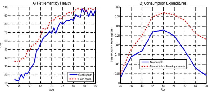
Panel A of Figure 2 presents retirement pro…les by age and health status, using 2000 data from the Health and Retirement Study (HRS). The percentage of individuals who report that they are in fair or poor health ("Poor health" in the …gure) and are retired is uniformly higher than that of retired individual in good, very good and excellent health ("Good health"). Moreover, almost 90% of all individuals in poor health between 55 and 85 years of age are retired, compared with only 43% of those in excellent health.
Finally, it is well documented that lifecycle consumption expenditures have a hump shape with a steep drop after retirement (Banks et al., 1998). Aguiar and Hurst (2005, 2008) show that the consumption drop at retirement is a fall in expenditures not associated with a fall in consumption because of the substitution between market goods and home production at retirement. People earn less income after leaving the labor force but they have more (non-market) time, so that they can spend more time shopping, preparing meals, etc. In other words, as the relative price of their time falls, individuals will substitute away from market
11Both studies, for methodological reasons, are not subject to "justi…cation bias" (Anderson and
expenditures and use more of their time to produce consumption goods. Hence, once one considers home production, the lifecycle consumption pro…le is much smoother. Panel B of Figure 2 presents consumption estimates from Aguiar and Hurst (2008).
50 55 60 65 70 75 80 85 90
10 20 30 40 50 60 70 80 90 100
A) Retirement by Health
Age
(%)
Good health Poor health
30 35 40 45 50 55 60 65 70
0 0.05 0.1 0.15 0.2 0.25 0.3 0.35 0.4
B) Consumption Expenditures
Age Log dev iat ion from age 25 Nondurable
Nondurable + Housing services
Figure 2: Retirement by health status (HRS, 2000) and Consumption Pro…le (Aguiar and Hurst, 2008)
3
The model
3.1
Demography
The economy is populated by a continuum of mass one agents who may live at most T
periods. There is uncertainty regarding the time of death in every period so that everyone faces a probability t+1 of surviving to the age t + 1 conditional on being alive at age t:
This lifespan uncertainty entails that a fraction of the population leaves accidental bequests, which, for simplicity, are assumed to be distributed to all surviving individuals in a lump-sum basis. The age pro…le of the population, denoted by f tg
T
t=1; is modeled by assuming
that the fraction of agents at aget in the population is given by the following law of motion
t= (1+gtn) t 1 and satis…es
T
P
t=1 t
= 1; wheregn denotes the population growth rate.
0otherwise. They know hs at the beginning of each period, but future health outcomes are uncertain. Indeed, an individuals’ health status is assumed to evolve over time according to a …rst-order Markov process with transition probability matrices t = [ t(hst; hst+1)], where
t(hst; hst+1) = Pr(hst+1jhst):
3.2
Preferences
In each period of life, individuals are endowed with one unit of time, which can be split among leisure, time spent in the labor market,lw;t;and time spent in home production, lh;t.
Individuals enjoy utility over consumption, ct; and leisure, 1 lw;t lh;t; and maximize the
discounted expected utility throughout life:
E
" T X
t=1
t 1
t
Y
k=1
k
!
u ct;1 lw;t lh;t
#
(1)
where is the intertemporal discount factor andE is the expectation operator. The period utility is assumed to take the form of a standard Cobb-Douglas utility function:
u ct;1 lw;t lh;t =
h
ct(1 lw;t lh;t)1
i1
1 (2)
where denotes the share of consumption in the utility and determines the risk aversion parameter.12
Following Becker (1965), home production in our model is such that the consumption that individuals care about, ct; is an aggregation of market purchased goods, ct; and time
spent in home production, where the aggregator is given by a CES function parameterized as follows:
ct=
h
&ct + (1 &)lh;ti
1
(3)
We allow for preference heterogeneity in time devoted to work at constant consumption and wage levels. In particular, we follow Kaplan (2011) and assume that = 1
1+ {hs;where
follows a log-normal distribution with mean
_
and variance 2:13 The shock is realized
at birth and retained throughout live. This additional source of heterogeneity is intended to take into account variations in work hours that are independent from the variations observed
12The coe¢cient of relative risk aversion with this utility speci…cation is given by: cu
in wages, which may be important for the study of retirement since it allows individuals with similar earnings and shocks history to exhibit di¤erent patterns of retirement behavior.
Note that individuals’ health status a¤ects preference for leisure. Indeed, it says that, on average, healthy agents (i.e., hs = 1) have stronger preference for work than do unhealthy ones (i.e., hs = 0): This relationship between the health condition of individuals and their willingness to work is useful to allow the model to replicate the di¤erence in the pattern of hours worked observed in the data between healthy and unhealthy agents.
3.3
Individuals’ problem
3.3.1 Budget Constraint
In our model economy, individuals make decisions about labor supply and asset accumula-tion. Because labor is endogenous, employment status is de…ned in terms of how many hours an individual works. In particular, individuals are considered to be participating in the labor force at age tif they supply at least 5% of their time endowment to the labor market and as not working or out of the labor force if they spend less than 5% of their time endowment in the market.14 In addition, as they reach the age of T
r and older, they may decide whether
to apply for retirement bene…ts. Thus, the age Tr is the earliest age at which a worker can
start collecting social security bene…ts in our model.
Individuals’ labor productivity is determined by an age-e¢ciency index denoted bye(zt; t) =
exp(zt+ t);in which tis a deterministic experience pro…le for the mean of earnings, andztis
a random component, which evolves according to an AR(1) process given byzt='zzt 1+"t
with innovations "t N(0; 2"); and thus accounts for the persistence in lifecycle earnings.
Labor productivity shocks are independent across agents and, as a consequence, there is no uncertainty over the aggregate labor endowment even though there is uncertainty at the individual level.
All workers in this economy pay labor income taxes ( w; ss), where the revenue from ss
is used to …nance the bene…t payments to the retirees, and w …nances overall government
expenditures not related to the social security system. Given that there is a maximum bene…t that a retired agent may receive, we consider an upper limit ymax on the taxable income, 14Considering one model period as one year, the threshold of 5% is equivalent to 300 hours a year, assuming
following the Social Security legislation. Thus, after-tax labor income for an individual who supplies labor lw;t is given by:
yt= (1 w)wlw;te(zt; t) ssminfwlw;te(zt; t); ymaxg+# (4)
where # is an exogenous lump-sum transfer component that captures the progressivity of the tax system.
Individuals incur medical expenses during each period, which are treated as necessary consumption that generates no utility but must be paid. Such expenses amount to out-of-pocket costs and insurance premiums. Following Hubbard et al. (1995) and French and Jones (2011), we model health costs as an exogenous drop in individuals’ resources. Empirical evidence in French and Jones (2004) shows that the cost of medical care increases with age and is correlated with individuals’ health status. In addition, they …nd that it exhibits high persistence over time and is very volatile as well. Based on this evidence, we model healthcare costs as:
met =q(t; hst; t; ut) (5)
where( t; ut)accounts for the idiosyncratic component of the medical expenses uncertainty,
in which t follows an AR(1) process given by t = ' t 1 + t with t N(0; 2) and
ut N(0; 2u) denotes the transitory component.
Individuals can resort to self-insurance to protect themselves against the uncertainty on labor income and medical expenses. Indeed, besides choosing the amount of time to supply to the labor market, they can trade an asset subject to an exogenous lower bound on asset holdings. We assume that this asset, which is denoted byat;takes the form of capital.
Thus, savings may be precautionary and allow partial insurance against idiosyncratic shocks. Agents are not allowed to incur debt at any age, so that the amount of assets carried over from age t to t + 1 is such that at+1 0: Furthermore, given that there is no altruistic
bequest motive and death is certain at age T + 1; agents who survive until age T consume all their available resources, that is, aT+1 = 0:
share of retirees, mainly the early ones, end up reentering the labor force following retire-ment.15 The importance of departing from the absorbing state assumption lies in the fact
that it may lead the model to understate the expected value of retirement, as some retirees would be better o¤ if they were allowed to go back to work.
As already said, individuals aged Tr and over are allowed to apply for social security
bene…ts. Let b(tr; x) = q(tr)bn(x) denote these bene…ts, where tr is the age at which the
application takes place and x is the average lifetime earnings, which is calculated by taking into account individual earnings up to age Tr. We specify the following law of motion forx:
xt+1 =
xt(t 1) + minfwlw;te(zt; t); ymaxg
t ; t= 1; :::; Tr (6)
The functionbn(x)is the bene…t that agents are entitled to at the normal retirement age.
It is a piecewise linear function, which is speci…ed in accordance with the rules of the U.S. social security system:
bn(x) =
8 > > <
> > :
1x if x y1
1y1+ 2(x y1) if y1 < x y2 1y1+ 2(y2 y1) + 3(x y2) if y2 < x ymax
(7)
where 0 3 < 2 < 1 and (y1; y2; y3) are the bend points of the function.
Thus, up to an average earning level of y1; individuals are entitled to 1x, so that 1
corresponds to the retirement replacement rate in this case. If the average past earnings are greater than y1 but smaller than y2; they will earn 1y1+ 2(x y1); and …nally if the past
earnings are greater than y2 but below ymax, bene…ts will be given by 1y1+ 2(y2 y1) + 3(x y2):
The function q(tr) captures how the retirement bene…ts are reduced or increased as
individuals start receiving them before or after the normal retirement age,Tn
r. In particular,
we have that:
q(tr) =
8 <
:
1 +ger(tr Trn)if tr 2[Tr; Trn]
(1 +gdc)(tr Tn) if tr 2(Trn;
_ Tr]
(8)
15Ruhm (1990) shows that about 25% of workers reenter the labor force following retirement. Nearly 70%
Thus, for each year that agents anticipate their bene…ts, they will face a linear reduction in their entitlements by a rate ofger:In contrast, bene…ts will be increased by a rate ofgdcfor
each year individuals postpone their receipt of social security bene…ts after reaching the full retirement age, Tn
r. However, this increase no longer applies when they reach age
_
Tr > Trn;
even if they continue delaying retirement.
We allow individuals to apply for social security bene…ts and continue to work, but those that choose to do so may face the retirement earnings test. Considering that the function of the social security bene…ts is to partially replace lost earnings, the retirement earnings test aims to prevent workers with relatively high earnings from receiving the bene…ts. The test withholds one dollar in bene…ts for each $2 of annual earnings above an exempt amount for individuals aged tr 2 [Tr; Trn) and $3 for those aged tr 2 (Trn;
_
Tr]. Formally, the earnings
test can be written as follows:
RETt=
8 <
:
b(tr; x) max(yt 2yret;Tr;0) for tr 2[Tr; Trn)
b(tr; x) max(yt 3yret;Tn;0) for tr 2(Trn;
_ Tr]
(9)
where yret;Tr and yret;T n are the threshold above which the test applies.
Additionally, in our model economy government provides individuals a minimum con-sumption, c after medical expenses are paid. We assume that transfers, tra, are conditional on individuals’ available resources. In particular, following Hubbard et al. (1995), we specify:
trat=maxfc+met [1 +r(1 k)]at yt RETtdss;t;0g (10)
where is the lump-sum transfers due to accidental bequests and dss;t = 1 if the individual
has applied for social security bene…ts, dss;t = 0 otherwise.
This equation implies that government transfers …ll the gap between an individual’s “liquid resources” - which may include not only their wealth and labor income, but also other government transfers such as social security bene…ts - and the consumption ‡oor. Thus, individuals can always consume at least c, even when their disposable resources fall short of covering their out-of-pocket medical expenses. The equation (10) is intended to be a model counterpart for means-tested programs such as Food Stamp, AFDC, Section 8 housing assistance, Medicaid and SSI.
economy is:
at+1 = [1 +r(1 k)]at+yt+ +trat+RETtdss;t met (1 + c)ct (11)
3.3.2 Recursive formulation of individuals problem
LetVw;t(st)denote the value function of antyear old agent, wherest= (at; ; zt; t; ut; xt; hst)2
S is the individual state space, and letVtr
ss;t(st) for t=Tr; :::; T denote the value function of
an individual agedtwho has applied for social security bene…ts at agetr:In addition,
consid-ering that agents die for sure at ageT and that there is no altruistic link across generations, we have thatVT+1(sT+1) = 0. Thus, the choice problem of individuals aged t= 1; :::; Tr 2
can be recursively represented as follows:16
Vw;t(s) = M ax lw;lh;a0 0
:
"
u(c;1 lw lh) + t+1 X
hs0
t(hs; hs0)EVw;t+1(s0) #
(12)
subject to (11) and (6), where s0 = (a0; ; z0; 0; u0; x0; hs0):
Whereas the problem of individuals aged t=Tr 1; :::; T can be written as:
Vw;t(s) = M ax lw;lh;a0 0
:
"
u(c;1 lw lh) + t+1 X
hs0
t(hs; hs0)EmaxfVw;t+1(s0); Vss;tt+1+1(s
0 )g
#
(13) where Vtr
ss;t(s)is given by:
Vtr
ss;t(s) = M ax lw;lh;a0 0
:
"
u(c;1 lw lh) + t+1 X
hs0
t(hs; hs0)EVss;ttr +1(s
0 )
#
(14)
subject to (11), wheres0 = (a0; ; z0; 0; u0; x; hs0):
Solving the dynamic programs in(12);(13)and(14);we obtain decision rules for the time spent in the labor market and the time spent in home production dlw;t , dlh;t : S ! [0;1],
asset holdings da;t :S !R+, consumption dc;t :S !R++; and for the decision of applying
for Social Security retirement bene…ts, dss;t : S ! f0;1g: Note, however, that individuals
may only apply for bene…ts at aget Tr:Additionally, once they apply, they are not allowed
to forsake the bene…ts, which means that if dss;t 1 = 1; then dss;t = 1:
16To simplify the notation, we have suppressed the subscript for age from both the state and control
3.4
Government
In our economy, the government manages a social security system, wherein the pension bene…ts to pensioners are …nanced through an exogenous tax ss. The amount of bene…t
received by each retired agent depends on his or her individual average lifetime earnings through a concave, piecewise linear function, which was presented above. Additionally, the government levies proportional taxes on consumption, c, labor income, w; and capital
income, k;to …nance an exogenous stream of expenditures, G, government transfer and the
servicing and repayment of its debt, D. We allow c to adjust to ensure that government
budget constraint is satis…ed at equilibrium. Finally, we assume that the government collects the accidental bequests and transfers it to all agents in the economy on a lump-sum basis.
3.5
Technology
The technology in this economy is given by a Cobb-Douglas production function with con-stant returns to scale, which is speci…ed byY =K N1 where 2(0;1)is the output share
of capital income, and Y,K and N denote aggregate output, capital and labor respectively. This technology is managed by a representative …rm, which behaves competitively in the sense that it picks capital and labor to maximize its pro…t, taking prices as given. Thus, the problem of the representative …rm can be written as follows:
=M ax
K;N :K N
1 wN (r+ )K (15)
where is the depreciation rate of capital.
Thus, the …rst-order conditions of the …rm’s maximization problem are:
r = K
N 1
(16)
w = (1 ) K
N (17)
3.6
Equilibrium
de…ned on subsets of the state space S: Let (S; (S); t) be a space of probability, where
(S) is the Borel algebra on S: Thus, for each ! (S); t(!) denotes the fraction
of agents aged t that are in !: The transition from age t to age t+ 1 is governed by the transition function Qt(s; !); which depends on the decision rules and on the exogenous
stochastic process for(z; ; u; hs): The functionQt(s; !)gives the probability of an agent at
aget and state s to transit to the set! at age t+ 1.
De…nition 1 Given the policy parameters, a recursive competitive equilibrium for this
econ-omy is a collection of value functionsfVw;t(s); Vss;ttr (s)g;policy functions for individual asset
holdings da;t(s); for consumption dc;t(s) for labor supply at the market dlw;t(s) and at home dlh;t(s), Social Security bene…t claiming decisions dss;t(s), prices fw; rg, age dependent but
time-invariant measures of agents t(s); transfers and a tax on consumption c such that:
1) fda;t(s); dlw;t(s); dlh;t(s); dc;t(s); dss;t(s)g solve the dynamic problems in (12); (13) and
(14);
2) The individual and aggregate behaviors are consistent, that is:
K =
T
X
t=1
t
Z
S
da;t(s)d t D
N =
T
X
t=1
t
Z
S
dlw;t(s)e(zt; t)d t
3) fw; rg are such that they satisfy the optimum conditions (16) and (17);
4) The …nal good market clears:
T
X
t=1
t
Z
S
fdc;t(s) + [da;t(s) (1 )da;t 1(s)]gd t =K N1
5) Given the decision rules, t(!) satis…es the following law of motion:
t+1(!) = t(hst; hst+1) Z
S
6) The distribution of accidental bequests is given by:
=
T
X
t=1
t
Z
S
(1 t+1)da;t(s)d t
7) c is such that it balances the government’s budget:
c =
G+SSB+PT
t=1 t Z
S
trat(s)d t+rD krK wwN
C
where SSB is the social security balance andC denotes the aggregate consumption.
4
Data and calibration
In this section we describe the data used to calculate the model and the calibration proce-dures17. Initially, the model is calibrated by taking into account 2000 data, which is set as a
benchmark. Afterwards, we introduce into the model the changes observed in the economic environment between 1950 and 2000 and investigate whether our model can replicate some stylized facts regarding retirement behavior. Finally, we isolate the e¤ect of Social Security, of the aging population, of Medicare and of the individuals’ productivity pro…le and inves-tigate the relative importance of each of these factors to the changes in retirement behavior during the period.
4.1
Demography
The population age pro…le f tgTt=1 depends on the population growth rate gn, the survival
probabilities t and the maximum age T that an agent can live. In this economy, a period
corresponds to one year and an agent can live 81 years, soT = 81:Additionally, we assumed that an individual is born at age 20, so that the real maximum age is 100 years.
Given the survival probabilities, the population growth rate in 1950 and 2000 is chosen so that the age distribution in the model replicates the dependency ratio observed in the data. Thus, we set gn = 0:0125 for 1950 and gn = 0:0105 for 2000. These values generate
17The standard calibration procedure of overlapping generations models can be found in Auerbach and
dependency ratios of 12.13% and 17.27%, respectively. By modeling the age-population distribution in such a way that it replicates the dependency ratio in data, we can capture the large increase in the number of individuals eligible for social security retirement bene…ts over the period under study.18
Data on survival probability by age and by health status were extracted from Bell and Miller (2005) and French (2005). As Panel A of Figure 3 suggests, life expectancy has increased from 1950 to 2000, as the survival probability pro…le shifted up and to the right during this period. For example, conditional on being alive at age 20, the expected life span was 69 years in 1950 for an individual in good health condition, whereas this same agent was expected to live until nearly 75 years of age in 2000. Likewise, the longevity of a healthy individual aged 50 rose from 72 to approximately 78 years during the same period.
20 30 40 50 60 70 80 90 100
0.2 0.3 0.4 0.5 0.6 0.7 0.8 0.9 1
A) Survival Probability by Healthy Status
Age Healthy - 2000 Unhealthy - 2000 Healthy - 1950 Unhealthy - 1950
20 30 40 50 60 70 80 90 100
0 0.1 0.2 0.3 0.4 0.5 0.6 0.7 0.8 0.9 1
B) Probability of Having Good Health in t+1
Age Given good health in t Given bad health in t
Figure 3: Survival and Good Health Probabilities
The transition probability matrices t= [ t(hst; hst+1)]were constructed using estimates
from French (2005) for the probability of having good health int+1conditional on the health status int. Panel B of Figure 3 shows such probabilities for both cases: poor and good health in periodt. As one should expect, the probability of being healthy tomorrow decreases with
18The number of individuals eligible for social security bene…ts has also increased because of amendments
age and is far higher for healthy agents than it is for individuals with poor health today, which suggests high persistence of health shocks over the lifecycle.
4.2
Preferences and technology
Values of the preference parameters( ; ; _
; 2;{)are summarized in Table 2:The
intertem-poral discount rate, ;was set to1:On a yearly basis, this value is consistent with a capital– output ratio of 3.09. The parameters of the stochastic process of shocks on the preference for leisure (
_
; 2) are from Kaplan (2011) and we set = 3. For Cobb-Douglas preferences,
the coe¢cient of relative risk aversion is given by 1 + and the Frisch elasticity for leisure is given by 1 + : For an individual with =
_
, the values reported in Table 2 entail a value of 1:77 for the coe¢cient of relative risk aversion and of 0:59 for the Frisch Elasticity for leisure. These values are consistent with the empirical evidence in Auerbach and Kotliko¤ (1987), Rust and Phelan (1997) and Domeij and Flodén (2006).
The parameter { is calibrated so that the model replicates the di¤erence in the pattern
of hours worked between healthy and unhealthy individuals over the lifecycle. French (2005) shows that at any point in the life cycle, the e¤ect of health on working hours is sizeable, ranging from 10% to 20%. With a value for { of 0.20, the model yields that individuals
with poor health work, on average, 13% than do those with good health. Figure 4 shows the average hours worked among healthy and unhealthy agents for the benchmark case.
Table 2: Preferences and Technological Parameters
_
2 { c &
1.0 3.0 1.60 0.25 0.20 0.36 0.054 0.056 0.7 0.55
In representative agent models, given the capital income share and the depreciation rate, there is a one-to-one relationship between the parameter and the fraction of time that individuals spend working in the stationary state. In overlapping generation models with heterogeneous agents, however, this relationship is more complicated. In this case, the usual procedure used to choose is such that the average fraction of time that individuals spend working is consistent with the empirical evidence, which suggests a value of approximately 30%.19 In our model economy, because = 1
1+ {hs; average hours worked is governed by
_
and, given a value of 1:60for
_
; individuals devote 28.5% of their time to the labor market under the baseline calibration.
The parameter , which governs the elasticity of substitution between market goods and time spent in home production, is set to 0.55. This value is consistent with the estimates in Aguiar and Hurst (2007) who report a range of 0.50-0.60 for . Given = 0:55;the parameter
& is then calibrated so that the average time spent in home production in the model economy matches its counterpart in the data, which is nearly 10% of the time endowment according to the American Time Use Survey (ATUS).
The consumption ‡oor, c; which is the model counterpart for means-tested programs such as Food Stamp, AFDC, Section 8 housing assistance, Medicaid and SSI, is set to 17% of the average income of the benchmark economy. This value corresponds to nearly $6220 (in 2000 dollars) and is within the range of values found in the literature. Indeed, Hubbard et al. (1995) estimate a value of $7000 for c; which, in 2000 dollars, corresponded to nearly 19% of the average income in the US economy. Using a similar procedure, French and Jones (2011) …nd a value of $4380, which is nearly 12% of the average income in 2000.
20 30 40 50 60 70 80 90 100
0 0.05 0.1 0.15 0.2 0.25 0.3 0.35
Age
Good health Bad health
Figure 4: Average hours worked by health status - Model 2000
economic growth rate, g; is constant and consistent with the average growth rate of GDP over the second half of the last century. Based on data from Penn-World Table, we set g
equal to 2:7%, which yields a depreciation rate of5:4%.
4.3
Individual labor productivity
Each agent in this economy is endowed with an individual productivity level e(zt; t).
Fol-lowing Huggett and Ventura (1999), we specifye(zt; t) = exp(zt+ t);where t denotes the
age-e¢ciency pro…le and zt denotes the persistent shocks on earnings, with the underline
stochastic process being characterized by the parameters ('z; 2
"). Several authors have
es-timated similar stochastic processes for labor productivity.20 Controlling for the presence of
measurement errors and/or e¤ects of some observable characteristics such as education and age, the literature provides a range of [0:88;0:96] for 'z and of [0:10;0:25] for ". In this
article, we follow the estimates of Floden and Lindé (2001) and set'z and 2
" to be equal to
0:91and 0:016; respectively.
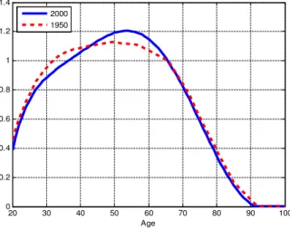
The values for tare constructed similarly to Huggett (1996) and MacGrattan and
Roger-son (2007). We use annual earnings and annual hours worked for the age groups 15-24, 25-34,..., 75-84 from IPUMS (U.S. Department of Commerce, Bureau of the Census 1950-2005). First, we construct hourly wages by dividing annual earnings by annual hours for each age group. Afterwards, we use a second order polynomial to interpolate the points to obtain the age-e¢ciency pro…le by exact age. We then truncate the polynomial to zero when it goes below zero which occurs at age 91 for 2000 and age 92 for 1950. Figure 5 shows the pro…les for 1950 and 2000 that are used in the calculations. The pro…les shown in the …gure are consistent with the empirical evidence provided by Heckman et. al. (2003) that shows that the e¢ciency indexes for older workers are smaller in 1990 than in 1950.21
20A revision of this literature can be found in Atkinson et. al. (1992).
21See also Ferreira and Pessoa (2007). We have not used the age-e¢ciency pro…les estimated by Heckman
20 30 40 50 60 70 80 90 100 0
0.2 0.4 0.6 0.8 1 1.2 1.4
Age 2000
1950
Figure 5: Age-e¢ciency pro…le
This fall in the relative productivity of older workers can be explained by technologi-cal progress. As shown in Sala-i-Martin (1996), changes in the technology of production have lowered the productivity of older workers thereby leading employers to replace them. Similarly, Graebner(1980) maintains that technological change leads to retirement because elderly individuals learn slower, making them obsolete in periods of faster innovation. 22
4.4
Medical expenses and Medicare
The out of pocket medical expenses function, q(t; hst; t; ut); is parameterized as follows:
q(t; hst; t; ut) = (t; hst) exp( t+ut) (18)
where the function (t; hst) captures the e¤ect of age and health on healthcare costs.
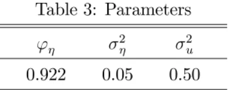
The parameters (' ; 2; 2
u) that characterize the idiosyncratic component of medical
expenses uncertainty are taken from French and Jones (2004). Table 3 reports the values of these parameters: As shown in the Table, the estimates from French and Jones reveal that not only are the shocks on medical expenses very persistent, but they are also quite volatile, with nearly 50% of the cross-sectional variance in spending being generated by transitory shocks.
22Blondal and Scarpetta (1999) also argue that the labor market for the elderly has worsened because of
Table 3: Parameters
' 2 2
u
0.922 0.05 0.50
We construct the age-health medical expenditures pro…le, (t; hst); for the benchmark
economy using the per person healthcare cost estimates by age reported in Meara et al. (2004). Based on data from …ve national household surveys they estimate per person spend-ing for 2000 and for the followspend-ing age groups: 5-14,15-24, 25-34,...,75+.23 We use a second
order polynomial equation to interpolate these points to obtain the age pro…le by exact age. The interpolated pro…le is displayed in Figure 6. Finally, we normalize the pro…le by dividing it by the average annual wage, which, according to the Social Security Bulletin (2001), was $36,564.
20 30 40 50 60 70 80 90 100
0 0.5 1 1.5 2 2.5
3x 10
4
Age Good health
Bad health
Figure 6: Medical expenses by age (US$) - 2000
We model the e¤ect of Medicare on retirement by investigating how it has changed the out of pocket medical spending function (18): Finkelstein and McKnight (2008) identify the e¤ect of Medicare on healthcare expenditures by comparing changes in spending for individuals over age 65 to changes in spending for individuals under age 65 between 1963 and 1970. To increase the plausibility of the identifying assumption that, absent Medicare,
23The 1963 and 1970 Surveys of Health Services Utilization and Expenditures; National Medical Care
changes in various types of spending for individuals above and below age 65 would have been the same, they focus primarily on changes in spending for the “young elderly” (ages 65 to 74) relative to spending for the “near elderly” (ages 55 to 64). The authors …nd that the introduction of Medicare is associated with a decline of 25% in the mean and of 16% in the standard deviation of out-of-pocket medical spending. In our context, these …ndings mean that, without Medicare, the out-of-pocket spending function (18) is shifted up for individuals aged 65 and over according tomet =f1met+f2;where the parametersf1 andf2
are calibrated in such a way that the new mean and variance of the distribution of healthcare costs capture the removal of Medicare.
4.5
Social Security and Taxation
The social security system in our economy is modeled so that it takes into consideration the main characteristics of the U.S. Social Security System. In 1950, the earliest age at which a person could receive Social Security retirement bene…ts was 65 so we set Tr = 46: After
1961, however, age 62 was adopted as an early retirement age, with reduced bene…ts. In our context, this point implies that Tr = 43 for 2000. The normal retirement age is the age at
which a person may …rst become entitled to unreduced retirement bene…ts. This age was 65 in 1950 and in 2000, so we have that Tn
r = 46 for both years.24
In the United States the old-age bene…t payable to the worker upon retirement at full retirement age is called the primary insurance amount (PIA). The PIA is derived from the worker’s annual taxable earnings, averaged over a period that encompasses most of the worker’s adult years. Until the late 1970s, the average monthly wage (AMW) was the earnings measure generally used. For workers …rst eligible for bene…ts after 1978, average indexed monthly earnings (AIME) have replaced the AMW as the usually applicable earnings measure. In our context, both AMW and AIME are given by (6).
The complete parameterization of the bene…ts function requires the speci…cation of values for the parametersf 1; 2; 3; y1; y2; ymaxg:The values used for each one of those parameters
are presented in Table 4. The parameters (y1; y2) correspond to the bend points applied in
the formula of calculation of the PIA, whereas ( 1; 2; 3) determine the replacement rate
applied in each one of the intervals de…ned by the bend points. For 1950, we use the bend
24The normal retirement age will increase gradually to 67 for persons reaching that age in 2027 or later,
points applied to calculate the PIA from creditable earnings after 1936 according to the Social Security Bulletin (2001). In this case, the PIA corresponds to 40% of the …rst $50 of AMW plus 10% of the next $200 of AMW. We multiply these values by 12, adapting to the annual base of the model and then normalize the result dividing it by the average annual wage.
Table 4: Bene…t Function Parameters
y1 y2 ymax 1 2 3
1950 0.23 - 1.13 0.40 - 0.10
2000 0.19 1.17 2.34 0.90 0.32 0.15
We follow a similar procedure for 2000. The values in this case correspond to those applied in the calculation of the PIA for workers who were …rst eligible in 1979 or later according to Social Security Bulletin (2001). In 2000, the PIA equaled 90% of …rst $531 of AIME, 32% of next $2671 and 15% of AIME over $3202. We again divide these values by the average annual wage.25
If individuals retire between 62 and 65 years old, their bene…ts are reduced by a formula that takes into account the remaining time to reach the normal retirement age. Thus, according to the Social Security Supplement (2001), if individuals retire at age 62, 63 or 64 they will receive 80%; 86:7% and 93:3% of the full retirement bene…t, respectively. Thus, we setger= 0:067:Conversely, social security bene…ts are increased by a given percentage if
individuals delay their retirement beyond the normal retirement age. This delayed retirement credit was instituted in 1972 to provide a bonus to compensate for each year past age 65 that a person delays receiving bene…ts, until age 70. Hence, gdc is equal to zero in our economy
in 1950. For 2000, we set gd equal to0:04; which is the delayed retirement credit for those
born in 1929-1930:
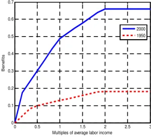
Figure 7 plots the bene…t function obtained for 1950 and 2000. The horizontal axis corresponds to the average past earnings,x;and the vertical axis corresponds to the bene…t. Note that we have normalized the average past earnings to the average labor income, ym.
Thus, for example, if an individual hasxequal toym;his bene…t would be equal to 17% of the
corresponding ym in 1950, whereas in 2000 it would be 42% of that value. It is immediately
25According to the Social Security Bulletin (2001), the average annual wage was $36,564 in 2000 and was
apparent from Figure 7 that bene…ts have become much more generous between 1950 and 2000.
Remember that ymax corresponds to the level of earnings above which earnings in
So-cial Security covered employment is neither taxable nor creditable for bene…t computation purposes. In 1950, the maximum taxable annual earning was $3000, whereas in 2000 it was $76200. We, then, divided these values by the average annual wage for both years to obtain
ymax=f1:13;2:34g; respectively.
Remember also that the parameter ssdenotes the contribution from workers to the Social
Security system. In 1950, American workers covered by the social security system contributed 3.0% of their wages to Old-Age and Survivors Insurance (OASI), which pays monthly cash bene…ts to retired worker (old-age) bene…ciaries, whereas in 2000 that contribution was 10.6%. Thus, we set ss= 0:03for 1950 and ss = 0:106 for 2000.26
0 0.5 1 1.5 2 2.5 3
0 0.1 0.2 0.3 0.4 0.5 0.6 0.7
Multiples of average labor income
B
enef
it
s
2000 1950
Figure 7: Bene…ts by multiples of average labor income
The amount exempted of the retirement earnings test for individuals aged 62-64 was $10,080 in 2000, whereas it was $17,000 for individuals aged 65-70. These values correspond, respectively, to 27% and 46% of the average wages in 2000. Thus, we set yret;Tr and yret;T n
to be 0:27ym and 0:46ym; respectively. We assume that there is no retirement earnings test
for the 1950 economy.27
26These values come from the Social Security Bulletin (2001) and are the combined employee-employer
tax for Old Age Social Security tax (OASI).
Finally, we specify the others parameters related to government activity. First, we set government consumption, G, to18%of the output of the economy under the baseline calibra-tion, whereas the ratio of federal debt held by the public to GDP is set at40%. We assume a labor income tax rate of14% and a capital income tax rate of 27%. The consumption tax is determined in such a way that the government budget balances in equilibrium, which implies a tax rate equal to 12%in the benchmark economy. These values are consistent with others retirement papers that also take into account a more general tax system (see, for example, Fuster el at., 2007). To calibrate the size of the lump sum transfer, #, we target the ratio of the Gini coe¢cient of after-tax earnings to the Gini coe¢cient of pre-tax earnings in the U.S.. According to Heathcote el at. (2010), this ratio was nearly 0.92, which yields a value of 0.045 for #:
5
Results
5.1
Benchmark Economy
The retirement rate by age in the model is given by the measure of agents at age t; t; who
are out of the labor force. Panel A of Figure 8 presents the retirement rate generated by the model for the benchmark case and the retirement pro…le observed in the U.S. economy in 2000. The model is able to reproduce very closely the retirement pro…le by age in 2000. In particular, it captures the jump in retirement at ages 62 and 65 and the relatively large number of individuals leaving the labor force before they reach the minimum eligible age for early bene…ts. Note that, in both the data and the simulation, almost 15% of the 55-year-old individuals were out of the labor force in 2000.
20 30 40 50 60 70 80 90 100 0
10 20 30 40 50 60 70 80 90 100
A) Individuals Out of the Labor Force (%)
Age Actual Data
Simulated
62 63 64 65 66 67 68 69 70
0 5 10 15 20 25 30 35 40 45 50 55
B) Distribution of Applications for SS Benefits (%)
Age
Actual Data Simulated
Figure 8: Model-data comparison for the benchmark economy - 2000
Our model is also able to reproduce very closely the pattern of applications for Social Security bene…ts. From Panel B of Figure 8 one can see that almost 48% of the total applications in the model economy occur at age 62, while the corresponding …gure in the data is 52%. Market incompleteness and the role of insurance played by Social Security bene…ts are very important to explain the high rate of claims at age 62. The peak in applications that takes place at age 65, in turn, is associated with the eligibility for full retirement bene…ts. In this case, the model yields a rate of 13.9%, while the actual value is 18%.
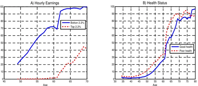
Figure 9 presents the retirement pro…le for the bottom and top 2.2% of the hourly earnings distribution, Panel A, and the retirement pro…le by health status, Panel B. The main message is that low earners and unhealthy individuals are much more likely to retire earlier than are their counterparts. As a matter of fact, for every age group, the retirement rate for individuals with low earnings is above that of the individuals with high earnings, as Panel A shows, which is consistent with the evidence in Table 1. According to the simulations, at age 62, nearly 90% of the individuals in the bottom of the distribution are out of the labor force, whereas 11% of the top 2.2% earners at the same age left the labor force.28
28Note that hourly earnings in our model are given bywe(z
t; t):Thus, the distribution of hourly earnings
45 50 55 60 65 70 0
10 20 30 40 50 60 70 80 90 100
A) Hourly Earnings
Age
Botton 2.2% Top 2.2%
30 35 40 45 50 55 60 65 70 75 80 0
10 20 30 40 50 60 70 80 90 100
B) Health Status
Age
Good health Poor health
Figure 9: Retirement by Hourly Earnings and by Health Status (%) - Model 2000
Likewise, up until the age of 75, the retirement pro…le of the unhealthy is always above that of the healthy individuals. Note also the steep jump in the retirement of the unhealthy at age 62, which is the minimum age for receiving Social Security bene…ts. These results are consistent with the empirical evidence in Section 2 and in Rust and Phelan (1997), which shows that individuals in poor health are roughly twice as likely to start collecting bene…ts at 62 rather than at age 65. This di¤erence exists because Social Security bene…ts provide a type of insurance against idiosyncratic shocks. Thus, in the presence of market incompleteness, which limits individuals’ ability to protect themselves against those shocks, lower income and unhealthy agents have a high incentive to apply for bene…ts as soon as they become eligible to secure a stream of income when it is needed. Additionally, given that the retirement replacement rate is decreasing with respect to the average past earnings, low income agents may …nd attractive to claim bene…ts earlier than the normal age even after considering the penalty for early applications.
fall because individuals are leaving the labor force, average non-market hours increase. This phenomenon occurs because, as noted in Section 2, as the relative price of their time falls, individuals will substitute away from market expenditures and use more of their time to produce consumption goods at home.
20 30 40 50 60 70 80 90 100
0.05 0.1 0.15 0.2 0.25 0.3 0.35 0.4 0.45 0.5
A) Consumption
Age
Market Expenditures Consumption
20 30 40 50 60 70 80 90 100
0 0.05 0.1 0.15 0.2 0.25 0.3 0.35
B) Hours
Age
Labor market Home production
Figure 10: Average consumption and the allocation of time over the life-cycle - Model 2000. In Panel A), "Consumption" corresponds to ct;which includes time spent in home production, while
we call "Market Expenditures" the variablect:
Finally, the second column of Table 5 shows some descriptive statistics for the benchmark economy. The table also shows values around which these statistics are found in the related literature. In terms of the distribution of labor earnings, wealth and consumption, the model economy is successful in approximating recent estimates for the U.S.. Burkhausera el at. (2004) report that the earnings Gini coe¢cient for all earners in 2000 was nearly 0.43, while the model economy generates a value of 0.405. Moreover, the model yields a substantially higher concentration of wealth than of earnings, as is the case in the actual data. Wol¤ (1994) reports wealth Gini coe¢cients of approximately 0.80, which is close to the simulated value under the baseline calibration. Finally, estimates in Garner (1993) suggest an actual consumption Gini coe¢cient near to 0.31, while this measure in the model is close to 0.3429. Overall, the model does a good job in reproducing the relevant statistics, 29The high level of wealth concentration generated by the model economy is largely due to the assumptions
and the "retirement facts" presented in Section 2.
Table 5: Descriptive Statistics
Benchmark Economy Literature Capital-Output Ratio 3.09 3.00 Gross Interest Rate 6.15% 6% Average Hours worked 0.28 0.31
Consumption tax 12% 8%
Gini Index - Earnings 0.41 0.43 Gini Index - Wealth 0.84 0.80 Gini Index - Consumption 0.34 0.31
5.2
Counterfactual Exercises
5.2.1 1950
To investigate how well the model explains the changes in retirement between 1950 and 2000, we introduced into the model the 1950 parameters, as described in the last section. Figure 11 presents the retirement pro…le generated by the model and the retirement pro…le observed in the data. The model is also able to replicate the pattern of retirement in 1950 quite well. Remember that the di¤erences between the 1950 and 2000 economies are the changes in the experience pro…le, changes in the demographic composition of population, modi…cations in the parameters relative to the social security system and the introduction of Medicare. As there is little left to be explained according to Figure 15, simulation results suggest that the changes in these variables account for almost all the observed change in retirement behavior over the period. Note also that, as it was the case in the 2000 simulation, labor force participation starts to decline after age 50 and the model is able to reproduce this fact, although its prediction slightly overstates this movement. In any case, the match after age 60 is very good.
Note also that the sharp decline in labor force participation at age 62 observed in 2000 is not present in the current simulation, which matches the data. Hence, this model simulation
shows that institutional changes related to social security are in fact e¤ective at in‡uencing retirement behavior. In this case, the introduction of early bene…ts between 1950 and 2000 created a peak in the distribution of social security applications in the latter year that was not present in the former.
20 30 40 50 60 70 80 90 100
0 10 20 30 40 50 60 70 80 90 100
Age Actual Data
Simulated
Figure 11: Individuals out of the labor force (%) - 1950
5.2.2 Accounting for the changes in retirement
In this subsection, we investigate the importance of each factor in determining the changes in retirement. In Panel A of Figure 12, we modify the benchmark case by changing the rules of Social Security to those of 1950, while keeping everything else constant. In Panel B, Medicare was eliminated (again, keeping all other parameters as in the benchmark case); in Panel C we feed the model with the 1950 demographic pro…le and in Panel D the age-e¢ciency pro…le of the benchmark economy is substituted with that of 1950.
20 30 40 50 60 70 80 90 100 0 10 20 30 40 50 60 70 80 90 100
A) Social Security
Age Benchmark - 2000 Changing Social Security
20 30 40 50 60 70 80 90 100
0 10 20 30 40 50 60 70 80 90 100 B) Medicare Age Benchmark - 2000 Eliminating Medicare
20 30 40 50 60 70 80 90 100
0 10 20 30 40 50 60 70 80 90 100 C) Demography Age Benchmark - 2000 Changing Demography
20 30 40 50 60 70 80 90 100
0 10 20 30 40 50 60 70 80 90
100 D) Age-efficiency profile
Age Benchmark - 2000 Changing Age-efficiency profile
Figure 12: Individuals Out of the Labor Force (%) - Model Simulations
the increase in retirement. Much the opposite, it has negative impact that, apparently, was compensated for by the changes in Medicare and Social Security. In fact, our simulation partly favors Bloom et al. (2007) as they show that, depending on social security provisions, improvement in life expectancy may increase working life.
In the simulation presented in Panel D the age-e¢ciency pro…le in the benchmark econ-omy is substituted with that of 1950. The impact in this case is not too large. For ages below 63, labor force participation falls, which is due to the fact that the age-e¢ciency pro…le in 2000 surpasses that in 1950 for ages 42-63. After that age, the impact is positive but small. This …ndings contrasts with Ferreira and Pessôa (2007), who found that this channel was a key force for the increase in retirement. Possible explanations for the di¤erent results are the fact that we use Census data and their calibration is based on CPS data and the introduction of Social Security and Medicare in our model.
Table 6 presents some of the numbers of the simulations of retirement rates for ages 62 to 68 in a di¤erent form. The second column presents the 2000 simulation ("Benchmark") and the last column presents the 1950 simulation, where all factors were changed at the same time. The remaining columns display the isolated impact (i.e., keeping all other factors constant at their 2000 values) of Social Security, Demography, Age-E¢ciency and Medicare, respectively, on retirement rate. The farther the number in one of these columns is from the 2000 value, the stronger the e¤ect of the corresponding factor.
For all ages, changes in Social Security have the strongest impact on retirement. For instance, the estimated retirement rate at age 62 when changing only the rules of Social Security is 31.9%, very close to the value of the full 1950 simulation30 (27.7%) and smaller
than that of all the other three cases. The isolated impact of Medicare is the second strongest. At age 65, for instance, the elimination of Medicare from the benchmark economy would
30Another way to see this result is as follows: if in 2000 the rules of Social Security were the same as in
cause a reduction in the retirement rate of almost twelve percentage points.
Table 6: Decomposition of the Changes in Retirement Rates
Age Variable Changed
Benchmark Social Security Demography Age-E¢ciency Medicare All (1950) 62 50.61 31.9 58.9 53.4 41.2 27.7
63 56.9 32.9 63.9 57.4 46.4 28.5 64 61.8 36.7 70.7 60.0 50.2 31.0 65 65.2 46.5 71.3 62.2 53.7 36.6 66 69.5 48.5 75.5 64.1 57.9 38.6 67 74.8 55.2 80.1 72.1 61.1 45.0 68 78.1 57.1 84.7 76.9 62.0 50.2
1Share of individuals out of the labor force (%).
As previously noted, changes in the age-e¢ciency pro…le between the two years had only a limited impact. As a matter of fact, for ages 62 and 63 its e¤ect goes in the opposite direction, and for all the remaining ages retirement rates are smaller than in the benchmark case. Finally, changes in the demographic pro…le imply that retirement rates in 2000 would be higher than the benchmark rates, for every age group, with the corresponding 1950 parameters.
5.2.3 Retirement Earnings Test and Delayed Retirement Credit
impact on higher earners than on lower ones, we show in Table 7 the change in the share of retirees aged 62-69 for the …rst and …fth quintile of the average past earnings distribution. As one can see in the Table, retirement decreases for individuals aged 65-69 in both cases but the fall is much larger for high earners. Indeed, the share of retirees aged 65, 66 and 67 in the …fth quintile is, without RET, 14.75%, 15.52% and 19.32% lower in comparison to the benchmark case, respectively, against 1.08%, 2.31% and 3.22% obtained among those in the …rst quintile.
Table 7: Change in retirement by past earnings (%) Age First Quintile without RET Fifth Quintile without RET
62 0.14 3.05
63 1.28 2.03
64 0.15 1.37
65 -1.08 -14.75
66 -2.31 -15.52
67 -3.22 -19.32
68 -4.21 -15.54
69 -3.85 -12.59
Finally, we also investigate the isolated impact of Social Security’s Delayed Retirement Credit (DRC) on the retirement of older men. The credit constitutes an incentive built into the program to promote work at older ages. It raises lifetime Social Security bene…t payments for recipients who delay receiving bene…ts beyond age 65. We use our model to investigate the impact of the DRC on retirement behavior and on claiming behavior. In particular, we run a counterfactual experiment in which we set gdc = 0: Table 8 shows the percentage
change in retirement and in the applications for Social Security bene…ts by age. The model predicts a small e¤ect of the DRC on retirement. This result should be expected because in our model economy retirement behavior is independent from the claiming behavior, which is more likely to be a¤ected by changes in the DRC. In fact, the third column of Table 8 shows a sizeable impact of DRC on the distribution of applications for social security. Bene…ts are now claimed much earlier, mainly at age 65: with gdc = 0; applications at age 65 increases