❊♥s❛✐♦s ❊❝♦♥ô♠✐❝♦s
❊s❝♦❧❛ ❞❡
Pós✲●r❛❞✉❛çã♦
❡♠ ❊❝♦♥♦♠✐❛
❞❛ ❋✉♥❞❛çã♦
●❡t✉❧✐♦ ❱❛r❣❛s
◆◦ ✻✽✸ ■❙❙◆ ✵✶✵✹✲✽✾✶✵
❚❤❡ ❊✛❡❝t ♦❢ ❙♦❝✐❛❧ ❙❡❝✉r✐t②✱ ❉❡♠♦❣r❛♣❤②
❛♥❞ ❚❡❝❤♥♦❧♦❣② ♦♥ ❘❡t✐r❡♠❡♥t
P❡❞r♦ ❈❛✈❛❧❝❛♥t✐ ●♦♠❡s ❋❡rr❡✐r❛✱ ▼❛r❝❡❧♦ ❘♦❞r✐❣✉❡s ❞♦s ❙❛♥t♦s
❖s ❛rt✐❣♦s ♣✉❜❧✐❝❛❞♦s sã♦ ❞❡ ✐♥t❡✐r❛ r❡s♣♦♥s❛❜✐❧✐❞❛❞❡ ❞❡ s❡✉s ❛✉t♦r❡s✳ ❆s
♦♣✐♥✐õ❡s ♥❡❧❡s ❡♠✐t✐❞❛s ♥ã♦ ❡①♣r✐♠❡♠✱ ♥❡❝❡ss❛r✐❛♠❡♥t❡✱ ♦ ♣♦♥t♦ ❞❡ ✈✐st❛ ❞❛
❋✉♥❞❛çã♦ ●❡t✉❧✐♦ ❱❛r❣❛s✳
❊❙❈❖▲❆ ❉❊ PÓ❙✲●❘❆❉❯❆➬➹❖ ❊▼ ❊❈❖◆❖▼■❆ ❉✐r❡t♦r ●❡r❛❧✿ ❘❡♥❛t♦ ❋r❛❣❡❧❧✐ ❈❛r❞♦s♦
❉✐r❡t♦r ❞❡ ❊♥s✐♥♦✿ ▲✉✐s ❍❡♥r✐q✉❡ ❇❡rt♦❧✐♥♦ ❇r❛✐❞♦ ❉✐r❡t♦r ❞❡ P❡sq✉✐s❛✿ ❏♦ã♦ ❱✐❝t♦r ■ss❧❡r
❉✐r❡t♦r ❞❡ P✉❜❧✐❝❛çõ❡s ❈✐❡♥tí✜❝❛s✿ ❘✐❝❛r❞♦ ❞❡ ❖❧✐✈❡✐r❛ ❈❛✈❛❧❝❛♥t✐
❈❛✈❛❧❝❛♥t✐ ●♦♠❡s ❋❡rr❡✐r❛✱ P❡❞r♦
❚❤❡ ❊❢❢❡❝t ♦❢ ❙♦❝✐❛❧ ❙❡❝✉r✐t②✱ ❉❡♠♦❣r❛♣❤② ❛♥❞ ❚❡❝❤♥♦❧♦❣② ♦♥ ❘❡t✐r❡♠❡♥t✴ P❡❞r♦ ❈❛✈❛❧❝❛♥t✐ ●♦♠❡s ❋❡rr❡✐r❛✱ ▼❛r❝❡❧♦ ❘♦❞r✐❣✉❡s ❞♦s ❙❛♥t♦s ✕ ❘✐♦ ❞❡ ❏❛♥❡✐r♦ ✿ ❋●❱✱❊P●❊✱ ✷✵✶✵
✭❊♥s❛✐♦s ❊❝♦♥ô♠✐❝♦s❀ ✻✽✸✮
■♥❝❧✉✐ ❜✐❜❧✐♦❣r❛❢✐❛✳
The E¤ect of Social Security, Demography and
Technology on Retirement
Marcelo Rodrigues dos Santos
Graduate School of Economics - Getulio Vargas Foundation
Pedro Cavalcanti Ferreira
yGraduate School of Economics - Getulio Vargas Foundation
Abstract
This article investigates the causes in the reduction of labor force participation of the old. We argue that the changes in social security policy, in technology and in demography may account for most of the changes in retirement over the second part of the last century in the U.S. economy. We develop a dynamic general equilibrium model with endogenous retirement that embeds social security legislation. The model is able to match very closely the increase in the retirement rate of males aged 65 and older. It also quanti…es the isolated impact on retirement and on the solvency of the social security system of the di¤erent factors. The model suggests that technological and demographic changes had a strong in‡uence on retirement, so that it would have increased signi…cantly even if the social security rules had not changed. However, as the latter became much more generous in the past, changes in social security policy can account not only for a sizeable part of the expansion of retirement, but also for the most of the observed increase in the social security expenses as a share of GDP.
Key words: social security; aging population; technology; retiment decision.
JEL classi…cation: D11; B12
We wish to thank Flávio Cunha, Rodrigo Soares, Carlos Costa and Samuel Pessôa and seminar partic-ipants at Paris1 and Cambridge for helpful comments. The authors acknowledge the …nancial support of CNPq-Brazil and Faperj. We are responsible for any remaining errors.
1
The E¤ect of Social Security, Demography and
Tech-nology on Retirement
1.1
Introduction
One of the most important economic changes that took place in the last century, particularly in the second half, was the reduction of labor force participation by old people. In 1950, 42% of men older than 64 years in the United States were working in contrast to only 17.5% in 2000. Just four out of every ten 66 year old male were retired in 1950, but …fty years later almost seven out of ten were out of the labor force. This phenomenon is hardly exclusive of the United States. Blondal and Scarpetta (1998) and Gruber and Wise (1999) provide evidence that the workforce participation of the old population has declined in many countries of the OECD.
The importance of understanding the factors that may account for this sizeable increase in retirement is that they may be in the root of the …scal crisis that the U.S. social security system is faced with today. In fact, according to the social security trustees 2002 report, in about 15 years the program will begin to experience permanent annual de…cits. As a consequence, it is projected that in 2041 the program will not be able to pay legally scheduled bene…ts.
Because coverage under the law has expanded and bene…ts have increased throughout most of this time period, the social security retirement system is an obvious suspect for the reduction in labor supply among the elderly. For a long time, economists have investi-gated the importance of higher social security bene…ts as an explanation for the changes in retirement using a variety of estimation methods.1 Nevertheless, the empirical evidence is
inconclusive. Parsons (1982) and Gustman and Steinmeir (1986), for example, have found that social security have had strong negative e¤ect on male labor supply, whereas Mo¢tt (1987), Burtless (1986) and Krueger and Pischke (1992) concluded that the large increase in real social security bene…ts over the past four decades had little e¤ect. These results suggest
1Surveys of the literature can be found in Diamond and Hausman (1984); Gustman and Steinmeier (1986);
that either there are problems associated with the methods that have been used to investigate this relationship, or there are other explanations that must be taken in consideration.
At the same time there was a marked changed in the demographic composition of the population in the U.S., namely, the aging of the population with the consequent expansion of the ratio of old to young people. In addition to obvious concerns on budgetary stability - as social security spending as a share of GDP tends to increase - the rise in longevity may play an important role in the decision to leave the labor force. Kalemli-Ozcan and Weil(2006), for instance, shows that exogenous decreases in the probability of death, which allows people to better plan saving for old age, generates longer retirement life.
Longevity may play an even stronger role in the decision to leave the labor force since the relative productivity of old workers have been declining in recent years at a faster pace than it used to. In fact, Heckman, Lochner and Todd (2003) provide evidence that old workers have become less productive relative to young workers over the second part of the last century. A technological explanation for this is most probable. Graebner(1980) argues that technical change leads to retirement because old people learn slower, making them obsolete in periods of faster innovation, such as the last twenty or thirty years. Moreover, because it reduces the opportunity cost of retirement and raises retirement bene…ts through increasing lifetime labor earnings, this change in the age-e¢ciency pro…le has an important e¤ect on the decision of leaving the labor force, as shown by Ferreira and Pessôa (2007).
This article develops and calibrates a stochastic overlapping generations model of large scale in order to investigate the causes of the observed change in retirement behavior of the American population between 1950 and 2000. We focus on the role of social security, of demographic factors (associated with higher longevity) and of changes in the experience pro…le. In the model, individuals decide at each period whether to stay in the labor force or to retire, by comparing the expected return of each option. If they continue working, they also decide how to divide their time between leisure and labor. The usual consumption/saving decision over all periods of the life cycle also applies. Government plays a simple role in this economy: it taxes individuals to …nance social security pensions.
then simulated taking into consideration the changes in social security, demography and age-e¢ciency pro…le between 1950 and 2000. The model simulations are able to reproduce very closely the retirement behavior in these two years. In particular, labor force participation of older males decreases to levels similar to those in the data. Moreover, the model is also consistent with the empirical evidence that older workers are working less hours.2
The present model is related to Rios-Rull (1996), Imrohoroglu, Imrohoroglu and Jones (1998), Huggett and Ventura (1999), Fuster et. al. (2006). These models provide a frame-work rich enough to deal with all the factors that potentially a¤ect the retirement decision. Besides, this structure allows us to model more accurately the dynamic structure of social security. In these papers, however, retirement decision is exogenous.
In Kopechy (2006), in contrast, the decision to leave the labor force is endogenous, but hours worked are …xed in every period and there is no social security in the model, which plays an important role here. As a matter of fact, we show that the single most important reason for the rise in the rate of retirement of old males by age is the increasingly generosity of the social security system. Also, of particular importance are the changes in the individual productivity pro…le, with longevity coming in third.
By endogeneizing the retirement behavior, our framework is also very convenient to study the impact of the aging population on the budgetary stability. In the one hand, higher longevity tends to expand the proportion of retirees and so the amount of bene…ts paid. This e¤ect of longevity arises through displacement of individuals toward states in which they are prone to retire. On the other hand, individuals, by living longer, give more weight to the future, which tends to raise capital accumulation, hours worked and, as a result, the output of economy.3 Hence, it is not clear beforehand what would be the net e¤ect. We show that
the aging of the population tends to put only a little pressure on the equilibrium of social security system …nances.
The paper also …nds that even if social security rules had not changed, total retirement would be considerably higher today than in 1950, especially because of demographic changes. However, the increase in the bene…ts paid-output ratio would be signi…cantly smaller than
2See, for example, McGrattan and Rogerson (1998).
3Moreover, as argued by Spriggs and Price (2005), the latter e¤ect tends to be ampli…ed if we take in
that observed in the data. In contrast, other groups of simulations show that the changes in the social security a¤ected much more the bene…ts paid-output ratio than total retirement, as bene…ts were now signi…cantly higher than in the past.
The last result is at odds with others in the literature (Krueger and Pischke (1992), for instance) that argue that the reduction of the retirement bene…ts would not impact the solvency of the system as it has little e¤ect on retirement. Hence, our analysis should serve as an useful point of reference for future proposals of social security reform: although the structure and the value of bene…ts are only one among many factors a¤ecting retirement decision, its quantitative impact on the solvency of the system is substantial.
The article is organized as follows. The model is presented in Section 2 and the calibration procedures and data in Section 3. In Section 4 results are presented and discussed; Section 5 concludes.
2
The model
In what follows we describe the overlapping generation model that will be used to guide our quantitative analysis of retirement. In this economy, individuals start working as soon as they are born. After spending a part of their life working, agents optimally decide whether or not to leave the labor force toward retirement. There is a social security system and the amount of retirement bene…ts that individuals are entitled to depends on their historical earnings. In order to obtain a smooth retirement behavior, we assume that individuals are faced with idiosyncratic productivity shocks.4 These shocks may also a¤ect the retirement
decision through the opportunity cost of leaving the labor force at a given age.
2.1
Demography
The economy is populated by a continuous of ex-ante identical agents who may live a max-imum of T periods. There is uncertainty regarding the time of death in every period so that each individual faces a probability t of surviving to the age t: Thus, a fraction of the
4Otherwise, if an agent decides to retire at a given age, all other agents will make the same decision. In
population leaves accidental bequest, which is distributed equally among all surviving indi-viduals. The age pro…le of the population f tg
T
t=1 is modeled by assuming that the fraction
of agents at the age t in the population is given by t= t
(1+gn) t 1 and
T
P
t=1 t
= 1; where gn
denotes the population growth rate.
2.2
Technology
The technology in this economy is given by a Cobb-Douglas production function with con-stant returns to scale: Yt = BKt (AtNt)1 where 2 (0;1) is the output share of capital
income, andY,K andN denote aggregate output, capital and labor respectively andB >0
is a constant scale parameter. The variableAdenotes a labor augmenting productivity index that grows a the constant rategA. The problem of the …rms is standard. They pick capital and labor optimally and the …rst order conditions are given by:
r = B K
AN 1
(1)
w = (1 )B K
AN (2)
where r denotes the net rate of return on capital, w the wage rate and the depreciation rate of capital.
2.3
Preferences
Each individual maximizes the discounted expected utility from consumption and leisure throughout life: E " T X t=1 t 1 t Y k=1 k !
u(ct;1 ht)
#
u(ct;1 ht) = c
1
t (1 ht) 1
1 (4)
where denotes the risk aversion parameter and denotes share of leisure in the utility.
2.4
Budget constrains
In each period of their life, individuals make decisions about work supply and capital ac-cumulation. When they reach the age of Tr and over they decide whether or not to leave the labor force. In our model, we set Tr to be the age in which the worker can apply for the social security system. While individuals are in the labor force, they earn a wagew and are submitted to idiosyncratic productivity shocks z. Let e(z; t) denote the e¢ciency index of an agent at age t with shock z; so that the labor earnings may be written as whte(z; t);
where ht denotes the labor supply.
All workers in this economy pay a tax to the government, which is collected to …nance the bene…t payment to the retired agents. Given that there is a maximum bene…t that a retired agent receives, we put a limit ymax on the taxable income, following the Social Security legislation. Thus, we can write the earnings of a worker at aget, after tax, as:
y(z; t; ; ymax) =whte(z; t) maxfwhte(z; t); ymaxg
We assume that workers also pay a lump-sum contribution which is used to balance the government budget at the equilibrium. Let at denotes the agent’s asset holdings at age
t, ct the consumption and the lump-sum transfer of accidental bequests and. Given these assumptions, we can write the budget constraint facing an individual who is in the labor force as:
(1 +gA)at+1 = (1 +r)at+y(z; t; ; ymax) + + ct (5) An agent agedTr and over may apply for social security retirement bene…ts. Letbt(tr; x)
denotes these bene…ts, where tr is the age at which the retirement decision takes place and
retirement bene…ts he has to leave the labor force and remains retired until the end of his life. Besides, the average of lifetime earnings is calculated by taking into account individual earnings up to ageTr. Thus, the law of motion for x can be written as:
xt= xt 1 (t 2) + maxfwht 1e(z; t 1); ymaxg
t 1 ; t= 2; :::; Tr (6)
Let Tn
r denotes the normal retirement age, that is, the age at which individuals can
claim full retirement bene…t. A worker that decides to retire at the agetr =Tn
r will receive bn
t(x; tr) =
~
b(x)
(1+g)t tr for the rest of his life. The speci…cation of the function
~
b(x)is based on the rules of the U.S. social security system:
~ b(x) =
8 > > > < > > > :
1x if x y1
1y1+ 2(x y1) if y1 < x y2 1y1+ 2(y2 y1) + 3(x y2) if y2 < x ymax
(7)
where 0 3 < 2 < 1.
Hence, up to an average earnings level of y1 retirees are entitled to 1x, so that 1
corresponds to the replacement rate. If the past earnings are greater than y1 but less than
y2; retirees will earn 1y1 + 2(x y1); and …nally if the past earnings are greater than y2
but less than ymax, retirees will be entitled to 1y1 + 2(y2 y1) + 3(x y2):
In our model, however, the age tr at which a worker decides to abandon the labor force and applies for social security retirement bene…ts may be less or greater than Tn
r. If
indi-viduals start their retirement bene…ts at the age tr 2 [Tr; Tn
r) then their bene…ts will be bt(tr; x) = trb
n
t(x; tr); where tr 2 [0;1]. In contrast, social security bene…ts are increased
by a rate gd if individuals delay their retirement beyond full retirement age. In this case, the retirement bene…t will be given bybt(tr; x) =bn
t(x; tr)(1 +gd)tr T
n
r:However, the bene…t
increase no longer applies when individuals reach age
_
Tr > Trn; even if they continue to
delaying retirement.
(1 +gA)at+1 = (1 +r)at+bt(tr; x) + + ct (8) Additionally, we assume that agents cannot have negative assets at any age, so that the amount of assets carried over from age t tot+ 1 is such that at+1 0: Furthermore, given that there is no altruistic bequest motive and death is certain at the age T + 1; agents who survive until age T consume all their assets at this age, that is, aT+1 = 0:
Finally, we are going to focus on the state steady of the economy under study. As a consequence, we have divided consumption, asset holdings, lump sum transfers and wage rate by Ain order to eliminate the e¤ect of economic growth. This transformation accounts for the term (1 +gA)at+1 in the individual budget constraints above.
2.5
Government
In our economy, the government manages a social security system, wherein the pension bene…ts to pensioners are …nanced by collecting tax from the current workers. This tax is assumed to be exogenous. The amount of bene…t received by each retired agent depends on his or her individual average lifetime earning through a concave, piecewise linear function, which was presented in the last subsection. The government does lump-sum transfers to the individuals in order to balance the bene…ts payment and the amount of collected tax. Furthermore, we assume that the government collects the accidental bequests which are also transferred on lump-sum basis for all individuals in the economy.
2.6
Equilibrium
Let s denote the individual states. It depends on the asset holdings a at the beginning of the period, on the lifetime average earnings x and on the idiosyncratic shock z so that
s= (a; x; z):LetVt(s)denote the value function of an agent in the workforce at the agetand
Vtr
t (s)the value function of an agent at the agetwhose the retirement age istr:The retirement
decision is such that an individual at the states retires at aget Tr ifVtr
t (s)> Vt(s);while
he or she remains in the labor market otherwise. The value functions Vt(s) and Vtr
de…ned by the following dynamic programs:
If retired :
Vtr
t (s) = max
a0 u(c;1) + t+1V
tr
t+1(s0) (9)
subject to (8)
where s0 = (a0; x; z)
If worker :
Vt(s) = max
h;a0 u(c;1 h) + t+1Ez0 max V
tr
t+1(s0); Vt+1(s0) (10) subject to(5); (6) and(7):
where s0 = (a0; x0; z0) for t Tr and s0 = (a0; x; z) otherwise.
Suppose A; X R+ andZ R; are the sets of possible values thata; x andz can take, so that we can de…ne the state space as S =A X Z: Letgt:S !R+ and %t :S !R+
be the policy functions associated with a0 and consumption, respectively, in the dynamic
programs (9) and (10), and nt : S ! [0;1] be the decision rule associated with h in (10). Finally, let 't:S ! f0;1g be the decision rule of retirement, which is de…ned as following:
't(s) =
8 <
:
1if Vtr
t (s)> Vt(s)
0otherwise
2.6.1 Recursive competitive equilibrium
At each point of time, agents are heterogeneous in regard to age t and to state s 2S. The agents’ distribution at age t among the states s is represented by a measure of probability
t de…ned on subsets of the state space S: Let(S; (S); t) be a space of probability, where
(S) is the Borel algebra on S: Thus, for each ! (S); we have that t(!) denotes
workforce or in retirement. Let w
t(!) denote the agents’ fraction at age t in the workforce
and rt(!) the agents’ fraction at age t in the retirement, so that t(!) = wt(!) + r t(!):
The transition from age t to age t+ 1 for individuals that are in the workforce is governed by the transition function Qt(s; !); which depends on the decision rule gt(s) of assets and on the realization of the idiosyncratic productivity shock z: The function Qt(s; !) gives the probability of an agent at aget and states to transit to the set!at age t+ 1. On the other hand, the transition of retired individuals is not stochastic and is just governed by gt(s):A recursive competitive equilibrium for this economy is de…ned as following:
De…nition 1 Given policy parameters f ; 1; 2; 3; y1; y2; ymax; Tr; Trng; a recursive
com-petitive equilibrium for this economy is given by fVr
t (s); Vt(s); gt(s); nt(s); b(tr; x); w; r; K; N; ; ; tg such that:
1) gt(s), nt(s) and 't(s) solve the dynamic problems(9) and (10); 2) The individual and aggregate behaviors are consistent, that is:
~ K = T X t=1 t Z S
gt(s)d t
N = T X t=1 t Z S
nt(s)e(z; t)d wt
3) fw; rg are such that they satisfy the optimum conditions (1) and (2);
4) The …nal good market clears:
T X t=1 t Z S
f%t(s) + [(1 +gA)gt(s) (1 )gt 1(s)]g=B ~ K N1
if 't+1(!) = 0
w
t+1(!) =
Z
S
Qt(s; !)d wt 8! (S)
if 't+1(!) = 1
r
t+1(!) =
Z
S
Qt(s; !)d wt 8! (S)
6) The distribution of accidental bequests is given by:
= T X t=1 t Z S
(1 t+1)gt(s)d t
7) Given that x follows the law of motion (6); bt(tr; x) satis…es (7);
8) is such that it balances the government’s budget::
= T X t=1 t Z S
wnt(s)e(z; t)d wt T X t=Tr t Z S
bt(tr; x)d rt
3
Data and calibration
In this section, we describe the data used to calculate the model and the calibration pro-cedures5. Initially, the model is calibrated taking into account 1950 data, which is set as
a benchmark. After this, we introduce into the model the changes observed in the eco-nomic environment between 1950 and 2000 and investigate whether or not our model is able to replicate the main retirement facts. Finally, we isolate the e¤ect of the social security, of aging population, and of the individual productivity pro…le and investigate the relative importance of each of these factors to the changes in retirement behavior in the period.
5The standard calibration procedure of overlapping generations models can be found in Auerbach and
3.1
Demography
The population age pro…lef tg T
t=1 depends on the population growth rategn, on the survival
probabilitiesstand on the maximum ageT that an agent can live. In this economy, a period corresponds to one year and an agent can live 61 years, so that T = 61: Additionally, we assumed that an individual is born with 20 years old, so that the real maximum age is 80 years old.
Given the survival probabilities, the population growth rate in 1950 and in 2000 is chosen so that the age distribution in the model replicates the dependency ratio observed in the data. Thus, we set gn = 0:0125 for 1950 and gn = 0:0105 for 2000. These values generate dependency ratios of 12.13% and 17.27%, respectively.
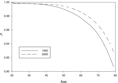
Data on survival probability were extracted from Bell and Miller (2005). As Figure 1 suggests, life expectancy increased from 1950 to 2000, as the survival probability pro…le shifted up and to the right in the period. In 1950, for example, life expectancy for an individual at age 20 was roughly 49 years old, while in 2000 it rose to 54 years old and for an individual at age 50 the life expectancy rose from 72 to 77 years old in the same period.
Figura 1: Survival Probability
Age
20 30 40 50 60 70 80
st
0,90 0,92 0,94 0,96 0,98 1,00
3.2
Preferences and technology
The values of the parameters related with the individual preferences( ; ; )are summarized in Table 1: The value of the relative risk aversion parameter follows the estimates of the microeconomic studies revised by Auerbach and Kotliko¤ (1987). The values supported by the empirical evidence are within the range [1;10]. In this study, we follow Auerbach and Kotliko¤ (1987) and used = 4.
In representative agent models, given the capital income share and the depreciation rate, there is a one to one relationship between the parameter and the fraction of time that individuals spend working in the stationary state. In overlapping generations models, however, such relation is more complicated because of heterogeneity among agents. In this case, the procedure used to choose is such that the average fraction of time that individuals in our model spend working is consistent with the empirical evidence, which suggests a value near 33%.6
Table 1: Preferences and technological parameters
~
β
γ
ρ
Bα
δ
gA1.003 4.00 0.61 0.90 0.36 0.056 0.02
In our model, since there is technological progress, the discount factor is given by =
~
(1+gA)(1 )(1 ):GivengA; and the parameter ~ is calibrated so that the capital-output
ratio in the benchmark economy is equal to 3.
The values of technological parameters (B; ; ) are also summarized in Table 1. We chose a value for based on U.S. time series data from the National Income and Product Accounts (NIPA).
The depreciation rate is given by:
= I=Y
K=Y gA n ngA
We set the investment-product ratio I=Y equal to 0.26 and the capital-product ratio
K=Y equal to 3.0. The productivity growth rate gA is constant and consistent with the average growth rate of GDP per capita over the second half of the last century. Based on data from Penn-World Table, we set gA equal to 2.00%. Thus, the equation above yields a
consistent with table 1.
Rios-Rull (1999) normalizes the value of parameter B; which measures the total factor productivity, in 1. In this paper, we follow Huggett (1996) so that we choseB to normalize the wage ratew in the benchmark economy: Thus, given a capital-product ratio of 3.0 and
= 0:36; the value ofB such thatw= 1 is 0.9.
3.3
Individual productivity
Each agent in this economy is endowed with an individual productivity level e(zt; t) = exp(zt+_yt); where
_
yt denotes the permanent component without risk that depends on age
and zt denotes a temporary component, which follows a …rst order auto-regressive process with parameters ( ; 2
"). Several authors have estimated similar stochastic processes for
labor productivity.7 Controlling for the presence of measurement errors and/or e¤ects of
some observable characteristics as education and age, the literature provides a range of
[0:88;0:96]for and of[0:12;0:25]for ". In this article, we followed the estimates of Flodén
and Lindé (2001) and set and 2
" to be equal to 0:91 and 0:0426;respectively.
The values for _ytare constructed following Huggett (1996). We utilize data from Current
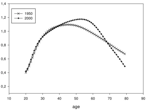
Population Reports on median earnings of full-time workers for each cohort. We have divided these values by the total median earnings and, then, interpolated to get the individual productivity component by age _yt. In Figure 3, we show the age-e¢ciency pro…le that is
utilized in our calculation for 1950 and for 2000. The pattern of change between 1950 and 2000 shown in the …gure is consistent with the empirical evidence provided by Heckman et. al. (2003) who show that the e¢cient indexes for old workers are smaller in 1990 than in 1950.
Figure 2: Individual Productivity by age
age
10 20 30 40 50 60 70 80 90
0,2 0,4 0,6 0,8 1,0 1,2 1,4
1950 2000
For computational reasons, we have approximated the AR(1) process which describes the idiosyncratic productivity shock z by a …nite Markov chain. First, we discretized the state space Z using a grid of 13 points equally spaced in the interval [ 3 z;3 z]; where z
denotes the unconditional standard deviation of z, that is, "=p(1 2): The transition
probabilities are computed using the algorithm described in Tauchen (1986). After calcu-lating the matrix of stochastic transition among the states inZ, we calculated the invariant distribution associated with this matrix and, then, took this result to describe the agent initial distribution in the economy.
3.4
Social security
The social security system in our economy is modeled so that it takes into consideration some important characteristics of the U.S. Social Security System, such as the dependence on retirement bene…ts to lifetime earnings.
was 65 so we setTr equal to 45 in the benchmark economy. After 1961, however, age 62 was adopted as an early retirement age, with reduced bene…ts. In our context, this implies that
Tr = 42 for 2000. The normal retirement age is the age at which a person may …rst become entitled to unreduced retirement bene…ts. This age was 65 in 1950 and in 2000, so we have that Tn
r = 45 for both years.8
If individuals retire between 62 and 65 years old, their bene…ts are reduced by a formula that takes into account the remaining time to reach the normal retirement age. Thus, according to the Social Security Supplement (2001), if individuals retire at age 62, 63 or 64 they will receive 80%; 86:7% and 93:3% of the full retirement bene…t, respectively. On the other hand, social security bene…ts are increased by a percentage if individuals delay their retirement beyond normal retirement age. This delayed retirement credit was instituted in 1972 to provide a bonus to compensate for each year past age 65 that a person delays receiving bene…ts, until age 70. Hence,gdis equal to zero in our economy in 1950. For 2000, we set gd equal to0:05; which is the delayed retirement credit for those who reached age 65 in 1997-1998:
In the United States the old-age bene…t payable to the worker upon retirement at full retirement age is called the primary insurance amount (PIA). The PIA is derived from the worker’s annual taxable earnings, averaged over a period that encompasses most of the worker’s adult years. Until the late 1970s, the average monthly wage (AMW) was the earnings measure generally used. For workers …rst eligible for bene…ts after 1978, average indexed monthly earnings (AIME) have replaced the AMW as the usually applicable earnings measure. In our context, both AMW and AIME are given by (6).
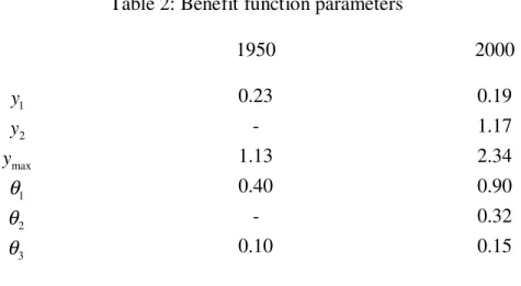
The function bt(tr; x) replicates the formula used to calculate the PIA. The complete parameterization of that function requires the speci…cation of values for the parameters
f 1; 2; 3; y1; y2; ymaxg: The values used for each one of those parameters are presented in table 2. The parameters (y1; y2) correspond to the bend points applied in the formula of calculation of the PIA, while ( 1; 2; 3) determine the replacement rate applied in each
one of the intervals de…ned by the bend points. For 1950 we used the bend points applied
8The normal retirement age will increase gradually to 67 for persons reaching that age in 2027 or later,
to calculate the PIA from creditable earnings after 1936 according to the Social Security Bulletin (2001). In this case, the PIA corresponds to 40% of …rst $50 of AMW plus 10% of next $200 of AMW. We multiplied these values by 12, adapting to the annual base of the model and then we normalized the result by dividing by the average annual wage.
Table 2: Benefit function parameters
1950 2000
1
y 0.23 0.19
2
y - 1.17
max
y 1.13 2.34
1
θ 0.40 0.90
2
θ - 0.32
3
θ 0.10 0.15
We followed similar procedure for 2000. The values in this case correspond to those applied in the calculation of the PIA for workers who were …rst eligible in 1979 or later according to Social Security Bulletin (2001). In 2000, the PIA equaled 90% of …rst $531 of AIME, 32% of next $2671 and 15% of AIME over 3202. We, again, divide these values by the average annual wage.9
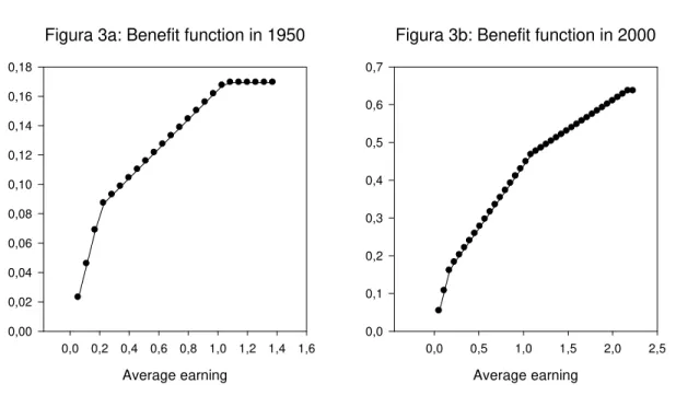
Figures 3a and 3b plot the bene…t function obtained for 1950 and for 2000, respectively. The horizontal axe corresponds to the average past earnings x and the vertical axe corre-sponds to the bene…t. We have normalized both …gures so that the average earnings in the economy, ym, is set equal to one:Thus, for example, if an individual has x exactly equal to
ym; his bene…t would be equal to 17% of the corresponding value in 1950. In contrast, his bene…t would be 42% of ym in 2000: Hence, it is immediate to see from Figures 3a and 3b that bene…ts have become much more generous between 1950 and 2000.
Remember that ymax corresponds to the level of earnings above which earnings in
So-9According to the Social Security Bulletin (2001), the average annual wage in 2000 was $36564 and in
cial Security covered employment is neither taxable nor creditable for bene…t computation purposes. In 1950, the maximum taxable annual earnings was $3000, while in 2000 it was $76200. We, then, divided these values by the average annual wage for both years in order to obtain ymax=f1:13;2:34g;respectively.
Figura 3a: Benefit function in 1950
Average earning
0,0 0,2 0,4 0,6 0,8 1,0 1,2 1,4 1,6 0,00
0,02 0,04 0,06 0,08 0,10 0,12 0,14 0,16 0,18
Figura 3b: Benefit function in 2000
Average earning
0,0 0,5 1,0 1,5 2,0 2,5 0,0
0,1 0,2 0,3 0,4 0,5 0,6 0,7
Finally, remember that the parameter denotes the contribution from workers to the social security system. In 1950, American workers covered by the social security system contributed with 3.0% of their wages for Old-Age and Survivors Insurance (OASI), which pays monthly cash bene…ts to retired worker (old-age) bene…ciaries, while in 2000 that con-tribution was 10.6%. Thus, we set = 0:03for 1950 and = 0:106 for 2000.
4
Results
The retirement rate by age in the model, r
t; is given by the measure of agents at aget that
are out of the labor force rt. In Figure 4, we display the retirement rate generated by the
who are in the labor force, leaving aside those who never participated of the labor force.10
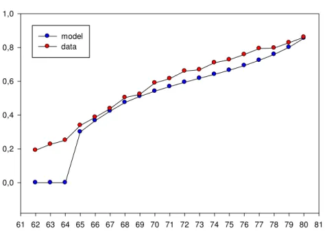
Especially for the individuals aged 65 and over the model is able to reproduce closely the retirement pro…le by age in 1950. In this year roughly 80% of workers older than 64 years had already left the labor force, hence the model gets a very good approximation of the overall retirement behavior of the American population in 1950.
Figure 4: Retirement rate by age for 1950
age
61 62 63 64 65 66 67 68 69 70 71 72 73 74 75 76 77 78 79 80 81 0,0
0,2 0,4 0,6 0,8 1,0
model data
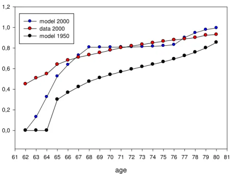
In order to investigate how well the model explains the changes in retirement between 1950 and 2000, we introduced into the model the data for 2000, as described in the last section. Figure 5 presents the retirement pro…le generated by the model and the retirement pro…le observed in the data, and we also display the simulated pro…le of 1950 for comparative purposes. The model is also able to match the retirement behavior for individuals aged 65 and over in 2000, and it is clear that the simulations capture the increase in retirement rate by age observed in the second half of the last century.
Note that the only di¤erences between the 1950 and 2000 economies are the changes in the experience pro…le, changes in the demographic composition of population and the modi…cations in the parameters relative to the social security system. As there is very little left to be explained according to Figure 5, simulation results suggest that the changes in these variables account for almost all the observed change in retirement behavior over the period.
Nevertheless the model does not have a good performance in explaining the retirement behavior for ages 62-64. A possible reason is that we have not taken in consideration the heterogeneity of health conditions among individuals. Rust and Phelan (1997) show that individuals in bad health are roughly twice as likely to receive Social Security at 62 as 65.11
These individuals have a higher disutility of work than those in good health. Thus, if there is market incompleteness, then the former will leave the labor force at the earliest age wherein they are entitled to receive retirement bene…ts. As we have homogeneity in regards to health condition at a given age, we are not able to capture this. Apart from this, the model is able to reproduce very closely retirement behavior in 1950 and 2000.
Figure 5: Retirement rate by age for 2000
age
61 62 63 64 65 66 67 68 69 70 71 72 73 74 75 76 77 78 79 80 81 0,0
0,2 0,4 0,6 0,8 1,0 1,2
model 2000 data 2000 model 1950
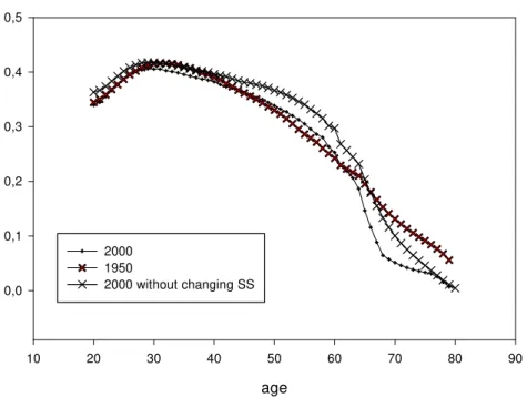
In Figure 6, we display the simulated labor pro…les by age for the benchmark case and for 2000. The model is also able to reproduce another stylized fact regarding labor decision, which is the fact that older workers are working less. McGrattan and Rogerson (1998) shows that work hours of people aged 65-74 and 75-84 have fallen about 57% and 70%, respectively, over the second part of the last century. In our simulations, the fraction of time that workers aged 65-74 spend working is about 54% smaller in 2000 than in 1950, while for workers aged 75-80 that fraction decreased 73% in the same period.
Feldstein (1974) argues that these drops in hours worked of older people could be ex-plained by changes in social security bene…ts. To investigate the e¤ect of social security on the labor supply, we also show in Figure 6 the result of a counterfactual exercise in which we maintain constant the parameters relative to the social security, but change everything else to their 2000 values. In this case, hours worked fall about 20% in the case of workers aged 65-74 and 68% for those aged 75-80. Thus, the model suggests that social security accounts for about 67% of the reduction in hours for workers aged 65-74 and about 10% for workers aged 75-80.
Moreover, the model suggests that the increase in social security bene…ts reduces the labor supply not only for the elderly, but over the whole working life. In fact, social security a¤ects the labor supply decision through the payroll tax and the level of bene…ts at retirement. When the latter becomes less generous, workers need to work more intensively at young ages in order to provide consumption at old age.12
12The econometric evidence on the e¤ect of social security on labor supply is inconclusive. For example,
Figure 6: Labor profile generated by the model
age
10 20 30 40 50 60 70 80 90
0,0 0,1 0,2 0,3 0,4 0,5
2000 1950
2000 without changing SS
Although the aggregate labor pro…le in Figure 6 is continuous, the individual labor pro…le generated by the model presents a discontinuity when individuals leave the labor force. In fact, one important feature of retirement is that workers make discontinuous transitions from full time work to not working at all. In order to reproduce this feature some authors have assumed that the agents in the economy supply labor indivisibly to the market while working.13 We have instead treated hours of work as a continuous choice variable. Even so,
we were able to reproduce the discontinuous transitions from full time work to not working through the discontinuous decision rule for retirement, which was described in subsection 2.6. In this case, agents decide whether or not to leave the labor force at age t based on which choice generates more utility for them. Hence, if the decision to retire at aget yields more utility than the decision to stay in the labor force, given the states, workers will leave the labor force and o¤er zero hours of work.
In Figure 7, we show the average consumption pro…le generated by the model in the benchmark case. According to evidence from Hurd (1980), among many, there is a drop in consumption at the time of retirement. Nevertheless, basic life-cycle models are not able to replicate this pattern since consumption in these models is smooth or even growing over lifetime. 14 In order to reconcile the empirical evidence with the theory, some authors
have argued that it is necessary to introduce into the basic life-cycle model the death risk (e.g., Davies (1981)) or/and an intratemporally non-separable utility (Attanasio and Weber (1993)). Our model includes these two hypotheses and, as a consequence, it is able to replicate the reduction in consumption at the time of retirement.
Figure 7: Average consumption profile - benchmark
age
10 20 30 40 50 60 70 80 90
0,2 0,3 0,4 0,5 0,6
4.1
Unraveling the channels to the changes in retirement
In this sub-section we investigate the role and measure the relative importance of the changes in the social security system, in demography and in the individual productivity pro…le to the changes in the retirement pattern.
14The problem appears when the discount factor is larger than 1 which is possible in models with …nite
In Figure 8 we show simulation results for changing one factor each time, keeping every-thing else constant. In order to analyze the e¤ect of each change, we also show in that …gure the retirement pro…le generated by the model in the benchmark case.
One can see that the changes in the social security system and in the experience pro…le over the time period under study shift up the retirement rate by age. On the other hand, the changes in demography shift down the retirement rate except for the oldest individuals. For instance, the retirement rate for 70 year old individuals in the benchmark case is 61%. As we change only the parameters of social security, the retirement rate of this group increases to 75%, while in the full simulation it goes to 81%. For the case in which everything is kept constant but the individual productivity pro…le is changed to its 2000 values, the increase in the retirement rate for this group is a little smaller, 75%. In contrast, retirement rate at age 70 falls to 60% for changes exclusively in demography.
Thus, the model suggests that the changes in government policy with respect to social security and in technology ( that changed experience pro…les) over the second part of the last century account for most of the changes in the retirement pro…le by age.
Kalemli-Ozcan and Weil (2006) have shown that the fall in mortality increases retirement. The idea is that the decision about labor supply over lifetime is a¤ected by uncertainty in regard to the date of death. If mortality is high, individuals who saved up for retirement would face a high risk of dying before he could enjoy their planned leisure and, as a result, they would plan optimally to work up to the end of their life. As the death risk falls, nevertheless, individuals would plan and save for retirement. According to Figure 8, our model suggests this “uncertainty e¤ect” is small and, in fact, appears only for individuals aged 75 and over. This result is due to the presence of the social security system, which provides insurance against the death disk.
everywhere above the full 2000 simulation. In other words, the delayed retirement credit is a powerful policy tool to induce workers to postpone their retirement.
Figure 8: Retirement rate for changing one factor each time
age
61 62 63 64 65 66 67 68 69 70 71 72 73 74 75 76 77 78 79 80 81 0,0
0,2 0,4 0,6 0,8 1,0 1,2
benchmark (1950) Demography experience profile social security
social security except gd
All data of 2000
It is well documented that there is a peak in retirement at age 65. Rust and Phelan (1997) suggest that the main reason for this are the rules of social security. In particular, the retire-ment behavior at age 65 would be strongly in‡uenced by the disincentive to continue in the labor force due to the retirement earning test - the rule that reduces social security bene…ts of those who have labor earnings above a certain threshold - and by the small incentive to continue working associated with the negligible delayed retirement credit.15 However, the
retirement earning test was abolished in 2000 for those between the full retirement age and 70 years of age and the delayed retirement credit has increased signi…cantly. Our model can be used to investigate the impact of these policy changes in the retirement behavior. Figure 9 shows the distribution by age of applications for social security produced by the model in two cases: the full simulation using 2000 parameters and another using 2000 parameters but leaving the delayed retirement credit unchanged, that is, gd = 0.16 It can be seen that the
15Rust and Phelan (1997) have set the delayed retirement credit equal to 1%.
16Notice that we have not taken into account the retirement earning test. Gustman and Steinmeier (2004)
increase in the delayed retirement credit reduces signi…cantly the peak in retirement at age 65. The model estimates that almost 40% of the applications would occur at age 65 with
gd = 0 as opposed to less than 20% with the new rules.17
Figure 9: Distribution of ages of application
age
61 62 63 64 65 66 67 68 69 70 71
0,0 0,1 0,2 0,3 0,4
changing all variables keeping gd constant
Table 3 displays further results on the e¤ects of the changes in social security legislation, demography and age-e¢ciency pro…le upon the aggregate retirement behavior and on the bene…ts paid-output ratio. The …rst column shows which factor was modi…ed in the simula-tion. The second shows the aggregate retirement rate - the ratio between retired population and total population - and the third column the total bene…ts paid-output ratio - social security spending as a share of GDP. Finally, the fourth column presents the sensibility of the total bene…ts paid-output ratio to the variations in the retirement rate.
Results in the table show that the changes in social security are the most important source of changes in aggregate retirement rate, following by changes in demography and in the age-e¢ciency pro…le, respectively. In fact, when only the parameters of the social security are modi…ed, aggregate retirement rate expands to 8.84%, accounting for 45% of the increase in the full simulation, 12.26%. The aggregate retirement rate goes to 8.23%
17The former result is close to that observed in a sample of individuals in good health conditions used by
in the case in which only demographic parameters are changed and 7.21% when only the age-e¢ciency pro…le is modi…ed (36% and 20% of all increase, respectively).
Thus, despite results suggesting that demographic changes have little e¤ect on the retire-ment decision at a given age, they have a strong impact on the aggregate retireretire-ment rate. This is so because aging population increases the concentration of individuals in states in which they are prone to retire.
Note also that the increases in retirement caused by changes in the social security have larger e¤ects on the bene…ts paid-output ratio than those caused by the other factors. In fact, one percentage point increase in retirement is associated with an expansion of 0.56 percentage point in the bene…ts paid-output ratio. This variation rate is signi…cantly smaller for changes in demography 0.09 and the age-e¢ciency pro…le 0.08.
In the last line, the simulation in which we changed demographic factors and experi-enced pro…le, but kept social security at the benchmark calibration, produced an aggregate retirement rate and a bene…ts paid-output ratio that are, roughly, 18% and 72% smaller, respectively, than in the full simulation. The previous …ndings allow one to conclude that if social security had not been changed, retirement would still be much higher in 2000 than 1950 (9.95% of the population, as opposed to 5.93%), but social security expenses as a share of output would be much smaller than otherwise (0.87% as opposed to 3.11%).
Table 3: Counterfactual experiments Variables changed in each
Simulation
Retirement rate = λ% Benefit total/output = b% ∆ ∆b/ λ
Benchmark (1950) 5.93 0.52
-All 12.26 3.11 0.41
Parameters of Social Security
8.84 2.16 0.56
Parameters of social security except gd
10.34 2.44 0.43
Experience profile 7.21 0.63 0.08
Demography 8.23 0.72 0.09
Experience profile and demography
Finally, we also show in the table results of a simulation in which all the parameters of social security were changed, except the delayed retirement credit, kept at its benchmark calibration. In this case the retirement rate jumps to 10.34%, and the bene…ts paid-output ratio to 2.44%. These values are above those of the simulation where all parameters of social security are changed, includinggd.
Note, however, that the sensibility of the bene…ts paid-output ratio to changes in retire-ment is lower in the former (0.43) than in the latter case (0.56). Whengdremains unchanged, social security spending as a share of output varies less proportionally than the retirement rate.
5
Conclusions
In this paper we have studied an stochastic life-cycle economy in which individuals pick optimally the time to leave the labor force. The model mimics relevant features of the American economy and takes special care in the calibration of the social security system. Simulations were able to match very closely the changes in retirement of American men aged 65 and over from 1950 to 2000.
The model suggests that the changes in demography, in technology and in social security may account for the most part of the variation in retirement over the time period under study. Furthermore, even if social security policy had not changed over time, retirement would still be higher, but the bene…ts paid-output ratio would be signi…cantly smaller. Although the aging population accounts for an important part of the increase in aggregate retirement rate, about 36% in our simulations, it is able to explain only a small part of the increase in the bene…ts paid-output ratio. In fact, the most important factor behind the sizeable increase in the social security expenses as share of output is the increase in retirement bene…ts.
6
Appendix: Computational details
convergence on the transfers of accidental bequest and capital. The algorithm for computing equilibria is as following:
1. Guess values for K0; 0; N; :
2. Use the …rst-order conditions of the pro…t maximization program of the …rm to obtain factor prices. The average income in the economy is then calculated and used to estimate retirement bene…ts.
3. Solve the dynamic programs of individuals in order to obtain the decision rules for assets, labor supply and retirement.
4. Use these decision rules to iterate on equilibrium condition 4 in order to obtain the age-wealth distribution.
5. Calculate K1; 1; N and . If K1 and 1 is approximately equal to K0 and 0;
respectively, stop. Otherwise, update K and and go to step 2.
We set a grid on the asset holdings a, on the past average earningsx and on the idiosyn-cratic shocks z: The number of grid points is 300, 40 and 13, respectively. The maximum value on the asset holding gridpoint is chosen such that the solution of the individuals’ dynamic problem is never biding. Also, the spacing between points on this grid increases with asset level.18 The points on the past average earnings grid are equally spaced and the
maximum taxable income for social security is taken to be the upper limit on this gridpoints. To calculate the individuals’ decision rules, we …rst use golden section search to solve labor supply as a function of initial and …nal asset level and, then, given the initial asset level, we iterate the value functions on asset gridpoints in order to …nd the optimal asset choice. Associated with this optimal asset choice, there is an interval at which the average earnings in next period belongs to. We interpolate the value function on this interval to obtain the …nal value function.
Finally, given individuals’ asset choices and the stochastic transition matrix on Z; the age wealth distribution is calculated through interaction on equilibrium condition 4.
18The points on the asset holdings grid are given bya
i= amax
3012
:35i
2:35
7
References
[1] Auerbach, A. and Kotliko¤, L. (1987), " Dynamic Fiscal Policy", Cambridge University Press.
[2] Atkinson, A.B. (1991). "The Distribution of wealth and The Individual Life Cycle". Oxford Economic Papers: No. 23, pp. 239-254.
[3] Attanasio, Orazio and G. Weber (1993). " Consumption Growth, the Interest
Rate and Aggregation". Review of Economic Studies 60, pp. 631-649.
[4] Bell F. and M. Miller (2005), "Life Tables for The United States Social Security Area 1900-2100". Social Security Administration: Actuarial Study No. 120.
[5] Blondal, S and S. Scarpetta (1999), "The Retirement Decision in OECD Coun-tries". OECD Economics Department WP 202.
[6] Burtless, G. (1986). "Social Security, Unanticipated Bene…t Increases and the Timing of Retirement". Review of Economic Studies: 53, pp. 781-805.
[7] Costa, D. L. (1998), "The Evolution of Retirement", The University of Chicago Press.
[8] Feldstein, Martin (1974), "Social Security, Induced Retirement, and Aggregate Capital Accumulation". Journal of Political Economy 82, pp. 905-26.
[9] Ferreira, P. C. and Samuel A. Pessoa (2007), "The E¤ects of Longevity and Distortions on Education and Retirement". Review of Economic Dynamic: Vol.10, No. 3, pp. 472-493.
[10] Floden, M. and Jesper Lindé (2001), "Idiosyncratic Risk in the United States and Sweden: Is There a Role for Government Insure?", Review of Economic Dynamics, Vol. 4, No. 2, pp 406-437.
[11] Gruber, J and D. Wise (1999), "Social Security Programs and Retirement
around the World". The University of Chicago, Chicago.
[12] Gustman, T. and T. L. Steinmeier (2004). "The Social Security Retirement
Earnings Test, Retirement and Bene…t Claiming". NBER Working Paper Series, 10905.
No 1, pp. 71-80.
[14] Heckman, J., L. Lochner and P. Todd (2003). "Fifty Years of Mincer Earnings Regressions" NBER Working Papers no 9732.
[15] Huggett, M. (1996). "Wealth Distribution in Life-Cycle Economies". Journal of Monetary Economics: Vol. 38, pp. 469-494.
[16] Huggett, M. and Gustavo Ventura (1999), "On the Distributional E¤ects of Social Security Reform". Review of Economic Dynamics 2: 498-531.
[17] Hurd, M. (1980). "Research on the Elderly: Economic Status, Retirement, and Consumption and Saving". Journal of Economic Perspective, 28(2), pp. 565-637.
[18] Hurd, M. and M. J. Boskin (1984). "The E¤ect of Social Security on Retirement in the Early 1970s". Quarterly Journal of Economics 99, pp. 767-790.
[19] Imrohoroglu, A., Imrohoroglu, S. and Joines, D. (1995), "A Life Cycle
Analysis of Social Security". Economic Theory 6, pp. 83-114.
[20] ______________ (1998), "The E¤ect of Tax-Favored Retirement
Ac-counts on Capital Accumulation". American Economic Review, 88(4): 749-768.
[21] Imrohoroglu, A., Antonio Merlo and Peter Rupert (2004), "What Accounts
for the Decline in Crime?". International Economic Review: Vol. 45, No. 3, pp. 707-729.
[22] Davies, James (1981). "Uncertain Lifetime, Consumption and Dissaving in Re-tirement". Journal of Political Economy, 89(31), pp. 561-77.
[23] Juster, F. T. and Frank P. Sta¤ord (1991), "The Allocation of Time:
Em-pirical Findings, Behavioral Models and Problems of Measurement". Journal of Economic Literature: vol. 29, No 2, pp. 471-522.
[24] Kopechy, K . A. (2006),"The Trend in Retirement", Meeting Papers 187, Society for Economic Dynamics.
[25] Kalemli-Ozcan, S and David N. Weil (2006), "Mortality Change, the
Uncer-tainty E¤ect and Retirement", Meeting Papers 28, Society for Economic Dynamics.
[26] Krueger, A. and Jorn-Ste¤en Pischke (1992). "The E¤ect of Social Security on Labor Supply: A Cohort Analysis of the Notch Generation". Journal of Labor Economics: vol. 10(4), pp. 412-437.
1950", Federal Reserve Bank of Minneapolis Quarterly Review, 22(1): 2-19.
[28] Ríos-Rull, J. V. (1996), "Life-Cycle Economies and Aggregate Fluctuations". Review of Economic Studies, 63(3): 465-489.
[29] Rust, J. and C. Phelan (1997). "How Social Security and Medicare A¤ect
Retirement Behavior in a World of Incomplete Markets". Econometric, vol. 65, No. 4, pp. 781-831.
[30] Sala-i-Martin, X. (1998), "A Positive Theory of Social Security", Journal of Economic Growth 1: 277-304.