FUNDAÇÃO GETULIO VARGAS
ESCOLA DE ECONOMIA DE EMPRESAS DE SÃO PAULO
BEATRIZ GRAVATO DE MATOS DE SOUSA ROCHA
THE INFLUENCE OF THE GLOBAL CRISIS ON THE SLOWDOWN OF THE EMERGING MARKETS
BEATRIZ GRAVATO DE MATOS DE SOUSA ROCHA
THE INFLUENCE OF THE GLOBAL CRISIS ON THE SLOWDOWN OF THE EMERGING MARKETS
Thesis presented to Escola de Economia de Empresas de São Paulo of Fundação Getulio Vargas, as a requirement to obtain the title of Master in Economy.
Knowledge Field: International Master in Finance
Adviser: Prof. Dr. Emerson Marçal
Rocha, Beatriz de Sousa
The Influence of the global crisis on the slowdown of the emerging markets / Beatriz de Sousa Rocha. - 2014.
51 f.
Orientador: Emerson Fernandes Marçal
Dissertação (mestrado) - Escola de Economia de São Paulo.
1. Dívida pública. 2. Crise financeira. 3. Mercados emergentes. 4. Fluxo de capitais. I. Marçal, Emerson Fernandes. II. Dissertação (mestrado) - Escola de Economia de São Paulo. III. Título.
CDU 336.3(81)
BEATRIZ GRAVATO DE MATOS DE SOUSA ROCHA
THE INFLUENCE OF THE GLOBAL CRISIS ON THE SLOWDOWN OF THE EMERGING MARKETS
Thesis presented to Escola de Economia de Empresas de São Paulo of Fundação Getulio Vargas, as a requirement to obtain the title of Master in Economy.
Knowledge Field: International Master in Finance.
Approval Date ____/____/_____
Committee members:
___________________________ Prof. Dr. Emerson Fernandes Marçal
___________________________ Prof. Dr. Martijn Franciscus Boons
ABSTRACT
This paper investigates the empirical relationship between the 2007-2009 financial crisis, the 2010-2012 sovereign debt crisis and the recent emerging equity markets slowdown. The exposure of the emerging markets to the crisis of the developed markets is quantified using an interdependence factor model. The results show that emerging markets did suffer a shock from both crisis, yet they recovered while the developed markets were still struggling. After the sovereign debt crisis emerging markets slowed down synchronized with the
developed market’s recovery. The paper further analyses whether capital flows
explain the connection between these two events, finding this relationship exists.
RESUMO
A presente dissertação investiga a relação empírica entre a crise financeira de 2007-2009, a crise da dívida soberana de 2010-2012 e a recente desaceleração dos mercados de capitais nos mercados emergentes. A exposição dos mercados emergentes à crise nos desenvolvidos é quantificada através de um modelo de interdependência de factores. Os resultados mostram que estes sofreram, de facto, um choque provocado por ambas as crises. No entanto, este foi um choque de curta duração enquanto os mercados desenvolvidos ainda lutavam com as consequências resultantes das sucessivas crises financeiras. A análise do modelo mostra ainda que após a crise da divida soberana, enquanto os mercados desenvolvidos iniciam a sua recuperação, os emergentes desaceleram o seu crescimento. De forma a completar a análise do modelo foi efectuado um estudo sobre a influência dos fluxos de capitais entre os mercados emergentes e desenvolvidos na direcção do seu crescimento, revelando que existe uma relação entre estes dois eventos.
Table of Contents
1. Introduction ... 8
2. Literature Review ... 9
3. The Interdependence Model ... 10
3.1. Model Estimation and Diagnostics ... 12
4. Model Results ... 17
4.1. Pre-Crisis, 2003 - 2006 ... 17
4.2. USA Credit Crisis, 2007 – 2009 ... 19
4.3. Eurozone Sovereign Debt Crisis, 2010 – 2012 ... 21
4.4. Post-Crisis, 2013 ... 24
5. Capital Flows ... 25
5.1. FPI Performance and the Interdependence Results ... 26
5.2. Equities Valuation ... 29
5.3. Foreign Investment and Currency Fluctuation ... 30
5.4. Capital Flows conclusions ... 31
6. Final Conclusions and main difficulties ... 33
7. References ... 37
8. Appendices ... 39
9. Appendices 2 ... 49
8
1. Introduction
In the late 80’s the emerging economies embarked in a liberalization process enabling the opening of the financial markets and the liberalization of the stock markets. Starting
at that moment the correlation with the developed economies increased substantially.
Even though many emerging markets (EM) are still not completely integrated within the
global markets (see Bekaert and Harvey (1995 and 2000) and Bekaert et al. (2011)),
relaxing the regulated barriers allowed the markets to extend its openness to the exterior
world, boosting the correlation between countries.
The relative contribution of the emerging markets to the world GDP over the developed
markets (DM) has been increasing. After the liberalization process the emerging
markets saw a sharp GDP growth, having almost doubled their weight on the global
economy (from 20% to 40%), while the developed markets share decreased from 80%
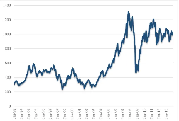
to 60% (see Figure 1 in appendix). The emerging equity markets development has been
turbulent due to the significant crisis the world have been through in the last 20 years.
After the shock the EM suffered with the 2008 financial crisis, it seemed like they were
recovering well. However, after 2012 the performance of the EM seems to almost
stagnate (see Figure 2 in appendix).
Given the increasing correlation between developed and emerging markets (see Figure 3
in appendix), the main goal of this project is to analyze if the slowdown of the EM was
a consequence of the global crisis. Therefore, to analyze this correlation, a four factor
model was developed to study the interdependence of a market with three external
factors and one domestic factor, aiming at finding if the emerging equity markets
9 crisis. The project focus on the periods before, during and after the crisis in order to
analyze how the interdependence between these countries changed over time.
Additionally, and in order to complete the previous analysis, a study on the relation
between the EM slowdown and possible movements of capital between developed and
emerging markets was prepared. The goal of this study is to investigate whether the
movements in foreign portfolio investment during and after the crisis influenced the
emerging equity market’s growth and slowdown.
2. Literature Review
There have been a number of empirical studies on global stock market crashes since the
seminal work of King and Wadhwani (1990) following the October 1987 Black
Monday. In a global context, international shock transmission has been widely
examined through the analysis on “contagion” and “Volatility spillovers” across borders
(e.g. Hamao, Masulis and Ng (1990); Baele (2005)). Both concepts aim at explaining
shock transmission that cannot be justified by fundamentals or excessive
co-movements. Several investigators have been studying how market integration promotes
contagion (Bekaert, Harvey and Ng (2005)) and when there was evidence of contagion
across borders as a consequence of financial crisis (e.g. Marçal, Pereira, Martin and
Nakamura (2009) and Marçal and Pereira (2009)). This project intends to analyze crisis
contagion to a specific group of countries. By adapting the model used by Bekaert,
Ehrmann, Fratzscher and Mehl (2012), that studies the global equity markets contagion
of the 2007-2009 financial crisis, the goal is to analyze how the 2007-2009 financial
crisis and the 2010-2012 sovereign debt crisis in the Eurozone affected the emerging
10
the model’ results with the capital flows between developed and emerging markets. As far as it is known the subject of correlations between capital flows in different countries
is not widely studied probably due to the limited data available. However, there are
studies on the correlation between foreign investment and exchange rate fluctuations
(e.g. Udomkerdmongkol, Görg, Morrissey (2006); Chakrabarti and Scholnick (2002)).
Therefore, based on that literature, on capital flows fluctuations over the years and on
other variables, this paper tries to establish a relationship between the equity markets
slowdown and the capital flows between DM and EM during and after the crisis.
3. The Interdependence Model
The methodology followed to construct the model used during this project was inspired
on the approach adopted by Bekaert, Ehrmann, Fratzscher and Mehl (2012) in analyzing
the contagion of the financial crisis into domestic portfolios. In particular, this project
focus only on the interdependence part of their model, specifically studying the
emerging markets and making some slight changes to their methodology.
The model estimated is an international factor model with four factors, where all of the
factors are capitalization-weighted market indexes. The model looks as follows:
𝑅𝑖,𝑡 = 𝑡−1[ 𝑅𝑖,𝑡] + 𝛽𝑖,𝑡′ 𝑡+ 𝑒𝑖,𝑡 (1)
= 𝑅𝑈 , 𝑅 𝑈 , 𝑅 𝐼𝐼𝐺 , 𝑅 (2)
Where Ri,t is the return of a domestic portfolio i during week t, Et-1[Ri,t] is the intercept
of the regression model assumed to be past expected values of future returns , Ft is the
11 The role of the domestic factor (RD) in the model is to explain all variation of returns
not explained by external factors. It was obtained by constructing a secondary portfolio,
different from the domestic index considered for portfolio i as the explanatory variable.
These secondary portfolios exclude therefore the securities that compose the dependent
variable.
Since the ultimate goal of constructing this model is to analyze the influence that the
global crisis had on the equity emerging markets’ returns, the external regressors being considered are representative of the developed markets that most suffered with the
crisis. By considering not just a US factor but also a EURO and a PIIGS (Portugal,
Italy, Ireland, Greece and Spain) factor we are aiming at finding which crisis within the
developed world influenced the EM economies the most; directly the 2007 – 2009 US credit crisis or the subsequent Eurozone sovereign debt crisis. For the same reason, and
in order to analyze if the interdependence relation changed over time, the model was
applied to different time periods, a pre-crisis period (2003 – 2006), a US crisis period (2007 – 2009), a sovereign debt crisis period (2010 – 2012) and finally a post-crisis period (2013). As already mentioned each factor and portfolio i inputs are the returns of
capitalization-weighted indexes1. The PIIGS factor was estimated as a weighted
average2 of the returns of the countries that form this group.
The returns are estimated as log returns and, in order to compute them, end of the week
stock prices in US dollars were collected from the Bloomberg database for each of the
1
The indexes representing the external country-factors are: S&P 100 (USA), EURO MSCI, PSI-20 (Portugal), ISEQ (Ireland), FTSE MIB (Italy), FTASE (Greece), IBEX (Spain).
2
12 indexes. The sample period goes from 1 January 2003 to 31 December 2013 and the
sample contains 574 weekly observations for the five country-representative portfolios.
As the final goal is to analyze the results of this model for the emerging markets, five
different models were constructed. A first one representing the EM in general, using for
that an index that measures the equity market performance of the global emerging
markets (MSCI Emerging Markets). Four other versions were calculated for each of the
BRIC countries (Brazil, Russia, India and China) 3, that were chosen as an example to
represent the emerging markets in a more detailed analysis of the interdependence
results. For each of these five versions, a model for each of the time intervals previously
mentioned was built.
With this model, the risk exposure of each of the portfolios being considered is captured
by the four factors. Under the null hypothesis, the interdependence between the
portfolios is determined by the factor exposure (β).
3.1.Model Estimation and Diagnostics
The interdependence model is a time series regression, or more precisely, a static model
given the nature of its variables. In this regression the independent variables are the
returns of the country representative-factors (vector F composed by three external
factors and one domestic factor) and the dependent variables are the returns of the
domestic portfolio i (i is representing each of the four BRIC and the EM MSCI).
Therefore, the method of ordinary least squares (OLS) was used to estimate the factor’s
exposure parameters (β). Each of the parameters will measure the partial effect of the corresponding independent variable (Ft).
3
13 A multiple regression model seems the most appropriate way to construct a model in
this situation given that it allows the independent variables to be correlated, making an
analysis where all the other factors are effectively hold fixed, while examining the effect
of a particular independent variable on the dependent variable. That is, analyzing the
ceteris paribus effect that a change in one of the country-factors, corresponding to the
developed countries, will have on the portfolios of emerging markets. However, no
independent variables can be constant neither can exist an exact linear correlation
between them, or the model would fall in the problem of perfect collinearity that would
bias the OLS estimations. There is some correlation between the country-factor
variables used for this model, for the time intervals studied, but there is no perfect
collinearity. Nonetheless, there are some pairs of variables that present excessively large
correlations that could still bias the results (see Table 1 in appendix). Therefore, the
model was corrected for that effect by eliminating the variables with lower statistical
significance from those pairs of variables presenting excess correlation.
In order to ensure that the OLS estimators are the best linear unbiased estimators
(BLUEs) and that the usual OLS standard errors, t statistics and F statistics can be used
for statistical inference there are five assumptions that the model needs to follow. This
procedure is called the classical linear model assumptions.
The first assumption states that the stochastic process4 must follow a model that is linear
in its parameters. The second one is about no perfect collinearity (already explained
above). The third one implies a zero conditional mean, indicating that for each t, the
expected value of the error ei,t, given the explanatory variables for all time periods, is
zero:
4
14
𝑒𝑡|𝑅𝑡𝑈 , 𝑅𝑡𝑈 , 𝑅𝑡𝐼𝐼𝐺 , 𝑅𝑡 = 𝑒𝑡| 𝑡 = 0 (3)
With the three previous assumptions it is already possible to establish the unbiasedness
of the OLS estimations. However, according to Goss-Markov, to ensure the estimators
are BLUE two additional assumptions were added: homoscedasticity and no serial
correlation.
The concept of homoscedasticity means that the standard deviations of the errors (ei) are
constant and do not depended of the independent variables. This procedure ensures that
each probability distribution for the dependent variables has the same standard
deviation, regardless of the independent variables. Is important to clarify that the
heteroscedasticity5 does not cause the OLS estimator to be biased or inconsistent but
can invalidate the error terms and test statistics.
Since heteroscedasticity is inherent to equity prices and the model uses log returns
calculated using the indexes’ stock prices, it is important to correct the model for the heteroscedasticity of the errors. Therefore, using the White covariance matrix estimator,
heteroscedasticity-consistent (White) standard errors were added to the parameter
estimates (In appendix 2 an example is displayed of the output of one of the versions of
the model, including a table with the White standard errors added to the parameters).
When estimating the model different model specifications were estimated. Starting with
the full model, including all independent variables, and step-by-step excluding the
variables with the least statistical significant parameters until only the significant
parameters with a 5% significance level were left. The aim of this approach was to
exclude the irrelevant variables to ensure the estimators were not biased. In addition and
5
15 as mentioned before this approach also helped in correcting for high correlations, as
well as in eliminating the variables that could cause the heteroscedasticity of the errors,
by selecting only those versions of the model that passed the
heteroscedasticity-consistent White test.
Due to temporal correlation in most time series data and since this is not a dynamic
model, it is very important to explicitly make assumptions about the temporal
correlation in the errors and about the relationship between the errors and the
explanatory variables in all time periods. Therefore, it is important to state that the
errors in two different time periods should be uncorrelated, conditional on the
independent variables (implying no serial correlation).
In order to ensure all the aforementioned assumptions were not violated, and to evaluate
the adequacy and performance of the model, besides some of the already mentioned
methodologies, the following steps were followed:
1) Analyze if the residuals plotted against the predicted values show no trends or
patterns. If any type of patterns such as a “cone” or a “sphere” shapes were found, the model was considered not fit and with unequal variances.
2) Examine the predicted values against the actual. If the predicted values seemed
extremely outside of the range of the response variable, it was considered as an
indicator that the model was incorrect for those cases. If the predicted values seemed
reasonable, the model was accepted assuming it was a good fit.
When the model is computed with several data samples it is possible that the model may
show signs of misspecification due to changing interdependences or to time-periods
16 of the model calculated and, from the 20 versions obtained, only one did not approve all
the tests: Russia for the time period 2003-2006. Consequently, this version will not be
considered for subsequent conclusions. (Appendix 2 contains a report with the tests
performed to one of the versions of the model as an example).
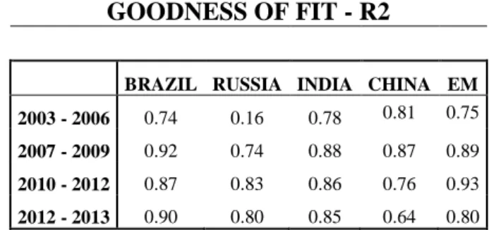
Before concluding the analysis of the model it is also important to measure its
goodness-of-fit looking at the R2 values, to be more precise, to the adjusted R2 as it
concerns a multiple regression. These values will indicate the proportion of the sample
variation of the dependent variable that is explained by the independent variables
collectively, ensuring the OLS estimation is a reliable estimation of the ceteris paribus
effects of each independent variable. For that reason, it can be said that this variables
are generally a good fit for this module since in the majority of the cases the adj.R2
ranges between 70% and 93%6 (see Table 2 in appendix). As observed in the Table 2 (in
appendix) there is also a lower value (16%), however this value belongs to one of the
versions of the models previously mentioned that did not passed the previous tests.
Therefore there is no reason for concern about this value.
Finally, in order to analyze if there is a relationship between the emerging markets’ returns and the factor’s returns the null hypothesis of the factor exposure being equal to zero (H0:β = 0) had to be tested, against the two-sided alternative of being different from zero (H1:β ≠ 0). Using a 95% confidence interval, it was concluded if the parameters were statically significant depending on the rejection of the null hypothesis.
The model created allows the study of the interdependence between a domestic portfolio
and the external portfolios. Therefore, if the hypothesis on whether the three first
6 The large adj.R2 are mainly caused by the domestic factor included in the model that should explain a great part of
17 parameters are zero (βi,US, βi,EURO, βi,PIIGS) could not be rejected, than no external influence on the dependent variables was considered to exist.
4. Model Results
During this section the results of the interdependence model previously presented are
interpreted. The first step is to identify which are the statistical significant parameters.
Table 3 (in appendix) contains only those statistically significant parameters for each of
the dependent variables selected to represent the emerging markets (BRIC indexes and
MSCI EM) for each time interval.
Looking into the results, it can be observed that, as it would be expected the domestic
factor is present in any time interval and in all the versions of the model. In contrast, the
same is not true for the influence of the other country-factors, which changes from
period to period and from portfolio to portfolio. Therefore, a more detailed analysis of
the results obtained was made. For this analysis it is important to evaluate the
parameters signs and values in order to quantify the magnitude and the direction of the
influence the country-factors will have on the emerging markets.
The following results in this section are based on US dollars returns for all the variables
included in the model. The same model was also computed with returns in local
currency but there were no significant differences in terms of the interpretation of the
results.
4.1.Pre-Crisis, 2003 - 2006
As it can be observed on Figure 2 (in appendix), this was a period of rapid growth of the
18 becoming more open to external markets after the liberalization process they went
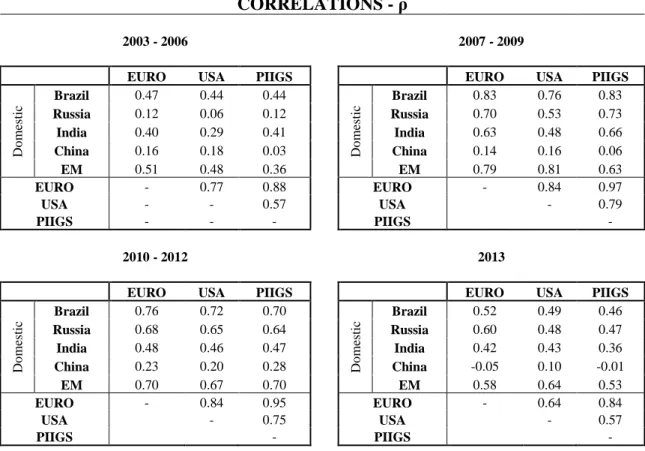
through, it makes sense that they show some interdependence with external factors. The
general index for EM shows interdependence with the USA (βEM, USA = 0.25) and with
PIIGS countries (βEM, PIIGS = 0.41). The model shows a positive parameter for those relations, which actually makes sense given the emerging stock markets growth and also
the USA and PIIGS stock markets growth at the same time. Between 2003 and 2006,
the USA was going through a period of expansion after the dot.com bubble crash
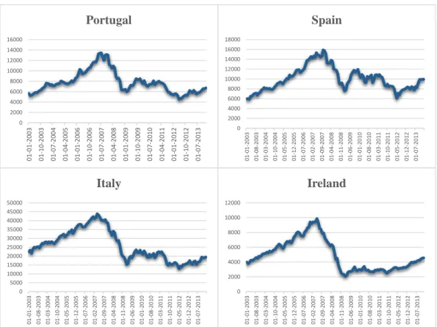
previously experienced around 2000. At the same time, countries like Portugal, Italy or
Spain faced consecutive years of stock markets growth (see Figure 4 in appendix).
On the other hand, when focusing on the BRIC countries, only Brazil, Russia and India
show evidence of external influence. Brazil presents a strong relation with the USA
(βBRAZIL, USA = 0.66) and a smaller relation with the PIIGS (βBRAZIL, PIIGS = 0.31), while
India presents interdependence only with the USA (βINDIA, USA = 0.23).
In the case of Russia, the results do not seem realistic as it is found a βRUSSIA, PIIGS = 0.85 jointly with a βRUSSIA, D = 0.05, meaning that Russia had been significantly more affected by external factors than domestic ones. In fact the model does not pass all the
fundamental assumptions previously mentioned, therefore it is not going to be taken
into account for the final conclusions. However, a possible explanation for the result of
this relationship with the PIIGS is that both markets were growing significantly at the
time. In 2005 the Russian stock market increased the number of stocks traded per day
by 90%. Between 2004 and 2005 thirteen IPOs and six secondary offerings occurred in
Russia, representing a combined value of $5.2bn in 2005 (see Goriaev and Zabotkin
19 showed an annual performance ranging from 0.19% to 80.17% between 2003 and 2006
(Morgan Stanley Capital International (2014)). At the same time, and as already
mentioned, the Italian, Portuguese and Spanish stock markets saw consecutive years of
growth. Therefore, a spurious relationship might be present in this case, meaning that
this interdependence coefficient might be wrongly inferred due to the coincidence of
both markets growth and to a confounding hidden factor. Since the Russian market was
opening to the exterior is possible that Russia was exposed to these markets, however it
does not seem very realistic to have such a strong interdependence with the PIIGS and
such a small interdependence with a domestic portfolio.
4.2.USA Credit Crisis, 2007 – 2009
The financial crisis of 2007 – 2009 was the hardest global financial recession since the Great Depression, according to the IMF’s 2008 World Economic Outlook. The origin of this crisis was in the USA due to a combination of factors such as a housing bubble,
easy credit conditions, subprime and predatory lending due to lack of regulation and
increasing financial engineering. Ultimately, all of these factors together led to the
collapse of several financial institutions and to a systemic collapse. Due to the severity
of the situation and to the equity markets global integration, the effects of this crisis
were spread way beyond the United States, leading to a serious global economic
recession in 2008. Therefore, the reaction of emerging markets to this recession is going
to be further studied.
Different results were found for this period for the five models created. First of all,
looking at the general EM results there are still external influences driven by the PIIGS
20 is high correlation between the PIIGS and the USA during this period, it is possible that
the PIIGS factor is capturing some of the relevance of the US factor exposure. Another
possible explanation for the coefficient’s results might be related with the exposure of the EM companies to these two groups of countries. The higher correlation of the EM
Index’ EPS (Earnings per Share) with the PIIGS’ EPS indicates the EM companies present more interrelationship with the PIIGS than with the USA (corrEM, USA=0.61;
corrEM, PIIGS=0.87).
The fact that there is still a significant factor exposure for the USA indicates that the
EM were affected by its financial downturn. Given that the sign of that parameter is
positive it suggests that the EM suffered a recession during this period, influenced by
the USA credit crisis. However, as the global peak of this financial recession was in
2008, it is possible that the positive returns of 2007, before the burst of the bubble,
might be causing the parameter to be small.
In the more detailed case of the BRIC countries there is not a homogeneous result.
China indicates no external influence, with the only significant parameter being the
domestic factor (βCHINA, D = 0.98). In the case of India, the model indicates only a
positive coefficient with the USA (βIndia, USA = 0.27), demonstrating it suffered the same effect previously explained for the EM in general. Russia indicates interdependence
only with the PIIGS (βRUSSIA, PIIGS = 0.54) and, finally, Brazil shows positive coefficients with both USA and PIIGS (βBRAZIL, PIIGS = 0.26 and βBRAZIL, USA = 0.22). Once again, as these two groups of countries present higher correlations in this period compared to
2003-2006 it is possible that the inclusion of both factors is dragging the corresponding
21 Concluding, during this period some of the emerging markets suffered directly the
negative shock of the USA crisis. However, the exposure parameters found were not
very high. As the peak of this crisis was in 2008, the positive returns of the pre-crisis
months of 2007 might be influencing the magnitude of the parameters. Additionally, the
recovery from the financial crisis was not synchronized between different markets
during 2009.
The results for the emerging markets and for each one of the BRIC were different.
These differences do not necessarily mean that the estimations are wrong. On the
contrary, since the emerging countries are not equally exposed to the USA they do not
suffer the shock uniformly. As the BRIC represent only four countries of the EM MSCI,
the interdependence parameter might be influenced by the other emerging market’s
performances. For example, the EM countries that have their currency pegged to the
dollar probably suffered a more intense shock, nevertheless is not the case of the BRIC,
since all have flexible/managed currencies.
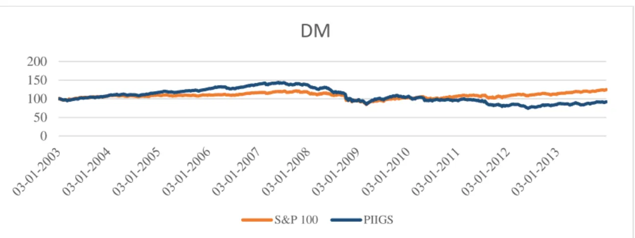
4.3.Eurozone Sovereign Debt Crisis, 2010 – 2012
Following the United States credit crisis, the Sovereign Debt crisis have been affecting
the Eurozone since 2009 when countries like Ireland and Greece started to face
difficulties in their banking systems. However, this crisis was brought to heel in 2010
when peripheral European countries required eminent bailout funds. At this time, a
sentiment of fear of financial contagion that could collapse the euro started to be felt
across all the European countries.
This crisis was characterized by a period of time in which several countries were facing
22 government securities. The rating agencies downgraded the government debt of several
Eurozone countries, having some of them arrived to a point of junk status. The countries
receiving funding were required to meet austerity measures to slow down the growth of
public debt, affecting several other economic sectors within those countries. The debt
crisis led to a crisis of confidence for European businesses and economies. This crisis
was however asymmetrical within Europe, where countries like Germany not only did
not suffer from it but were actually facing economic expansion. In this section is studied
the reaction of the EM to the European crisis given the correspondent exposure.
Using the EM general index as independent variable, the external parameters for the
EURO and PIIGS factors were statistically significant. However, as these two
parameters are highly correlated, in order to ensure that one was not capturing the
other’s influence, an individual analysis7 of each of them was computed. As a result the corresponding interdependence were βEM, PIIGS = 0.1 with the PIIGS and βEM, EURO = 0.14 with the EURO. Looking into the correlations on Table 1 (in appendix) one can see
that the domestic factor shows high correlation with two external factors, consequently
it might be capturing power out of the two external factors.
Nevertheless, despite presenting the same correlation with both the EURO and the
PIIGS, the interdependence coefficient with the EURO is slightly higher. A possible
explanation for this result might be related with the composition of the EURO MSCI
index that is representing the EURO countries. About 79%8 of this index is composed
by securities of the European countries that were least affected by the crisis. As already
mentioned this crisis mostly affected the periphery of Europe and 79% of the The
7
This analysis excludes the corresponding correlated factor but it still includes de domestic factor.
8The weight was calculated by the sum of each country’s securities weight in the index, from all composing
23 EURO MSCI depends on northern European markets that were rather facing an
asymmetric shock relatively to the periphery (see Table 4 and Figure 5). In addition, the
small magnitude of the parameters might also be related to the fact that EM started to
slow down around 2012 and those values might be influencing the parameter’s
magnitude. Concluding, the sovereign debt crisis caused only a limited impact on EM.
Meaning that, as the PIIGS saw a downturn in their markets, the EM did not have a
strong reaction in the same direction. On the other hand, it seems that the EM were
following closer other European countries rather than the underperforming PIIGS (see
Figure 5 in appendix).
In what concerns the BRIC countries, one can see that they are divided in two groups:
India and Brazil reveal positive parameters with the USA (βBrazil, USA = 0.33; βINDIA, USA = 0.3), while Russia and China show positive parameters with the EURO (βRussia, EURO = 0.22, βChina, EURO = 0.11). Nonetheless, both results can be interpreted the same way. As already mentioned the EURO MSCI as a whole was not facing a recession during this
period and the USA was already recovering from the previous crisis, therefore the EM
appear to be slightly following the countries that were least struggling, indicating they
did not suffer strong contagion from this crisis.
Contrary to the other BRIC, India appears to be following USA downturn and recovery,
as it is the only country showing positive coefficients with USA in both periods of
crisis.
To sum up, by the results shown by the model it seems like the EM did not suffer strong
24 that they were not infected by this crisis at all, as there were signs of contagion on the
EM index, though very small.
Looking at Figure 2 (in appendix) one can see that after 2009 the equity market
performance of the emerging markets still grew, allowing for the possibility that this
European recession may have boosted that growth with capital flows. Fearing the
European situation investors might have preferred to invest in emerging markets during
this period. Later in this paper will be performed a study on this specific subject.
4.4.Post-Crisis, 2013
As the developed markets are recovering from the consecutive crisis, it seems like the
Emerging markets are starting to show a slowdown. One can see that, despite the
bounced path of the equity emerging markets during the last six years, it appears they
are now suffering a slowdown in 2013 (see Figure 2 in appendix).
Looking at the model results one can see that the EM shows a negative parameter with
the PIIGS (βEM, PIIGS = -0.25) and a positive parameter with the EURO countries
(βEM,EURO = 0.32). The PIIGS faster growth and the negative coefficient found, indicate that the EM were underperforming, or at least growing at a much slower pace. Even
though the EM were not highly influenced during the time of the sovereign debt crisis,
it appears that they are now affected by the DM recovery.
These results leave open the possibility of an influence driven by capital flows. On one
hand, during the crisis capital inflows into EM may have influenced these economies
positively. On the other hand, since 2013 capital outflows might have influenced EM
25 Nonetheless, looking deeper into each BRIC the same results cannot be found. This
means that the EM-DM relationship was spread over the emerging countries in a
non-homogeneous way. From the model results, it appears that these countries only
presented positive interdependence with countries that were growing/recovering during
2013. In the case of China or India there are no signs of external influences.
5. Capital Flows
The first database of emerging markets’ equity returns was collected only twenty years
ago by the World Bank, for a conference on the “Portfolio Flows to emerging equity
markets”. At the time, the concept of Foreign Portfolio Investment (FPI) in EM was
relatively recent (as opposed to direct investment) and, with that conference, the World
Bank aimed at better understanding the risks that foreign portfolio investors faced in
emerging markets (Bekaert and Harvey (2014)). In this section, it is going to be
analyzed if the slowdown of the emerging markets was a cause of the movements of
capital between the FPI of the EM and the FPI of the DM that may have occurred
during and after crisis.
As mentioned in the previous section, the EM’s performance behavior during and after
the crisis opened two questions: What is making these equity markets grow as the DM
are suffering consecutive crisis? Why are currently the EM lacking on growth while the
DM are recovering? Therefore, in an attempt to answer these questions the paper
analyzes whether during the crisis there were capital flows leaving the developed
markets and entering the emerging markets boosting its equity markets growth. In the
26 there were capital flows in the opposite direction causing the slowdown of the emerging
equity markets.
Given that it was only possible to obtain yearly data on a period of 10 years, it would
not be reasonable to rely on correlations or models results with so few variables.
Therefore, the analysis will alternatively go through three different steps: 1) analyze the
growth rate of the FPI’s amounts jointly with the coefficients of exposure previously
calculated; 2) Go through the evolution of the EM’s equity valuations; 3) Study the
performance of the DM market against the EM currencies movements.
5.1.FPI Performance and the Interdependence Results
Firstly, yearly data9 of the outwards and inwards of Foreign Portfolio Investment for the
countries involved in the analysis was collected for the time period between 2003 and
2013. The paper analyzes the FPI amounts for the USA individually, while for the other
countries the FPI amounts are computed at group levels (EM and PIIGS), rather than at
individual country level. At the European level, only the PIIGS were analyzed since
these were the ones mostly affected by the sovereign crisis. At the EM level, FPI
amounts differed substantially between countries and, therefore, a more specific
analysis for i.e. the BRIC countries was left out.
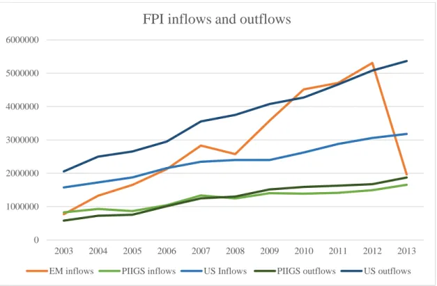
While every market was showing positive growth in its FPI inflows from 2006 to 2007
(the US increasing by 9%, the PIIGS by 28% and the EM by 33%), from 2007 to 2008
there was clearly a disturbance on portfolio investment worldwide. The PIIGS and the
EM’s net inflows10
decreased by 169% and 10%, respectively, and the US’s net inflows
9 All the data collected in US dollars.
10
27 decreased by 12%, meaning that even though inflows increased by 2% it was not
enough to surpass the amounts of outflows (see Figure 6 and 7 in appendix).
In the next period (2008-2009), while PIIGS and USA outflows were still growing and
causing negative net inflows (with the USA showing a 0% increase in the inflows and
9% increase in outflows, and the PIIGS experiencing a higher increase of 16% in its
outflows than in its inflows, 13%), EM’s net inflows rapidly recovered increasing by
44% (see Figure 7 in appendix). In the previous section it was found a positive
coefficient between the EM and the USA for the period of 2007-2009 indicating the EM
had suffered a shock linked to the US crisis. The small magnitude of the coefficient
suggested that it should have been a short-lived shock and, as it can be seen with the
FPI results, the EM recovered faster. These outcomes suggest that there might be a
possible connection between the DM increasing outflows and EM increasing inflows,
investors may have preferred to invest in the EM and consequently changed their capital
allocations geographically.
From 2009 to 2010 as the US inflows started to recover leading to an increase in net
inflows of 2%, PIIGS situation was becoming more dramatic with an additional 82%
decrease in net inflows and 5% increase in outflows. At this time, the EM net inflows
continued to show a positive growth of 28%.
As seen in the previous section, the EM proved to be exposed to the sovereign crisis,
although less than to the 2007-2009 financial crisis. This result can also be observed on
its FPI development. From 2010 to 2011, the EM net inflows still increased but at a
much smaller rate of 1%. This time the shock was different from the one suffered with
28 continue to grow and surpass its inflows, which seemed almost stagnated given the
minor changes, the EM continued to grow recovering its net inflows in 11% from 2011
to 2012.
From 2012 to 2013 the EM saw a sudden sharp decrease of 63% in its net inflows. At
this time US inflows were growing at 4% and PIIGS’s at 11% (representing an
acceleration of PIIGS flows when comparing with the previous year growth).
Additionally, the negative coefficient of exposure of the EM to the PIIGS found for
2013 also indicated they were moving in opposite directions. These results would
suggest that that there might be a connection between the DM’s global crisis recovery and the EM’s slowdown. However, when looking at Figure 7 (in appendix) one can see that during 2013 the USA and PIIGS net inflows continued to fall, meaning that its
outflows continued to overpass the inflows. In addition, the decrease in the EM FPI was
not only on the inflows but also on the outflows (decreased around 62% as well). The
aforementioned results consistently suggest that during the crisis period (2007-2012)
investors had geographically changed their preferences, nevertheless in the after crisis
period (2013) the same cannot be concluded. As there were actually less capitals leaving
the EM and the increase in the capitals entering the DM was not significant, it is not
possible to conclude there were in fact movements of capitals flying back to the DM
economies only based on this information. Actually, these results open the question on
whether the situation of the EM FPI in 2013 is a consequence rather than a cause of the
29
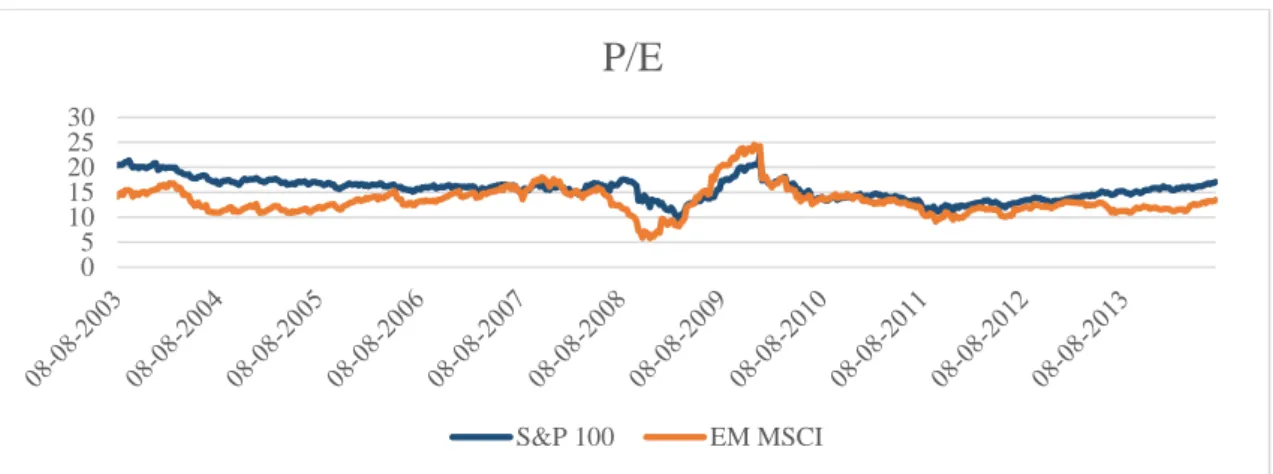
5.2.Equities Valuation
If there were capitals flying from the DM to the EM during the crisis, it would be
expected that the EM companies would increase their market value during this period.
According to the Institute of International Finance, after 2009 the price-to-book ratios of
EM equities were more expensive than the ones of DM companies. In an attempt to
corroborate that theory and analyze if the valuation of the EM companies had a positive
movement during the crisis, the P/E (price-to-earnings) ratios of both DM and EM
companies11 were calculated. The P/E (Price-to-Earnings) ratio indicates how much an
investor is willing to pay per dollar generated by the underlying company. Therefore, if
the EM P/E is increasing it means that the investors believe stronger on the
fundamentals behind these assets and consequently invest more on them.
Looking at Figure 8 (in appendix) one can see that the P/E of EM increased sharply
after dropping around 2008, overpassing the values for USA during 2009, suggesting
the EM equities were relatively more expensive than the US equities during this crisis
period, regarding the corresponding fundamentals. In the same way, looking at Figure 9
(in appendix) one can see that the same relation is true between the P/E of EM and the
P/E of PIIGS from early 2009 to mid-2010.
After 2012 the P/E of the EM decreased as the P/E of the US increased. Therefore,
suggesting investors were again putting more faith into DM equities and preferring to
invest in this group of countries. These valuations may indicate a geographic shift in
investors’ preferences in line with the previous analysis, suggesting a movement of
capitals during and after crisis.
11
30
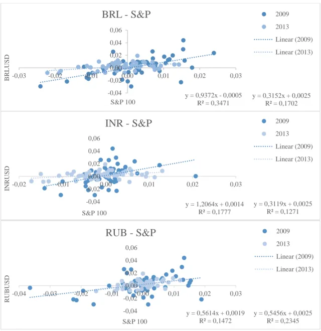
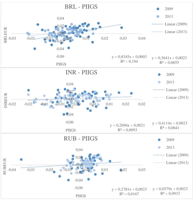
5.3.Foreign Investment and Currency Fluctuations
If there are foreign portfolio inflows into a country, there is commonly a demand for the
country’s currency. Empirical studies have proven that depreciated local currency
attracts foreign investment (e.g. Udomkerdmongkol, Görg, Morrissey (2006);
Chakrabarti and Scholnick (2002)). Increasing foreign investment represents increasing
currency demand and should be a pressure for relative change of value between both
countries, even though foreign portfolio investment may not be the main driver of a
currency relative valuation.12
The performance of the FPI inflows and outflows of DM and EM during and after crisis
was analyzed in previous subsections. In this subsection the performance of the DM
indexes with the EM local currency evolution is going to be compared. If there were
capitals leaving the DM contributing to a negative return of local equity markets and if
these capitals would be entering the EM, there could be a positive correlation between
the DM index returns and the EM foreign-exchange rates returns.
Given that this analysis aims to support the previous study of the FPI movements, it will
focus only on the periods to which the main relations were found. Therefore, it will
target 2009 when the distance between increasing net inflows of EM and increasing
outflows of DM was higher and 2013, when the EM suffered a strong shock in their
foreign investment. The BRIC individual currencies were used as example for EM
currencies.
12 The main drivers of currency appreciation and depreciation should be: relative product prices, monetary policy,
31 In Figures 10 and 11 (in appendix) are the scatter plots showing the correlation and the
linear regression between the variables being analyzed. As it can be seen, during 2009
all the foreign-exchange rates studied show a positive relationship both with the PIIGS
and the USA13. Meaning that as these two DM indexes were falling, the EM currencies
were appreciating. In some cases the R2 given by the scatter plots are very small. This is
expected since foreign portfolio investment is not a main driver of the currency
fluctuations. These result aligned with the fact that foreign portfolio inflows were
sharply increasing in EM during this period of time, suggests that there was a
geographic shift in the investor’s preferences to the EM.
For the after crisis period the same effect is present but with the inverse flow. It
suggests that the capitals were now flowing back to the DM as their indexes were
appreciating, while the EM foreign exchange currencies depreciated (in Figure 12 in
appendix the evolution of the performance of the DM can be observed, confirming it
was increasing in the period after crisis).
5.4.Capital Flows conclusions
According to the literature, EM have become “darlings” of international investors over the past decade, attracting capital to their fast-growing industries and delivering a boost
to the global economy (Sergie (2014)). However in contrast to developed economies,
investors are commonly not willing to accumulate their currency, meaning that if some
instability is starting to be felt capitals rush out the local currency to the DM. This
chain of events, leaves a great deal of devalued local currency and has already caused
crisis in several regions over the past decades (Sergie (2014)). Capital flows can be
13
32 inconsistent and after years of foreign portfolio inflows it can suddenly shift and
investment is dragged out of EM.
During the previous subsections it was possible to find that during the crisis
(2009-2012) net inflows of EM substantially increased as the DM’s decreased and the DM
outflows increased, suggesting there was a relation between the two. Afterwards, it was
possible to see that during the beginning of the same time period, the valuation of the
EM equities increased, indicating investors were valuing these equities more highly
during the crisis than before. In addition, a positive correlation was found between EM
foreign-exchange rates and the DM indexes, meaning that as the indexes were falling
the currencies were appreciating. The three aforementioned results together, indicate
that there was in fact a geographic change in investor’s preferences and, therefore, movements of capitals from the DM to the EM.
Looking into Figure 13 (in appendix), it is possible to see that according to the Morgan
Stanley Research Team (2013), a sharp rise in net portfolio flows towards DM equity
and debt markets supported EM currencies between 2009 and early 2011, thus
supporting the results previously found. Their theory adds that this portfolio flows are
being supported by QE (Quantitative Easing)14 and the growth differentials between the
EM and DM. However, they argue that as QE decelerates and growth differentials
narrow (according to their economists’ aggregated forecasts), portfolio flows will not
provide currencies the same level of support.
During the after crisis period (2013), the EM saw a sudden steep decrease in its net
inflows at the same time as the US and PIIGS inflows were growing. After 2012, the
14 QE is a monetary policy used by central banks to increase an economy money supply by purchasing government
33 EM P/Es decreased to values lower than the DM P/Es suggesting investors were now
pricing the EM equities lower and thus investing less. In addition, the relationship
between the DM indexes and the foreign exchange rates also suggests the investors
preferences returned to the DM. Therefore, even though the increase in the capitals
entering the DM was not significant and there was also a decrease in the EM outflows,
there is evidence that investor’s changed their preferences by stopping investing in the EM to invest back in the DM. This result is in accordance with what was said in the
previous paragraph, with the FED announcement of the tapering15, the portfolio flows
decreased not supporting the EM local currencies anymore.
Furthermore, the negative coefficient of exposure of the EM to the PIIGS found for
2013 also indicates the performance of the EM was negatively affected by the recovery
of the DM. Given that the EM show a negative coefficient with a group of countries that
was recovering at the time and that capitals were flowing from EM to DM, one can
conclude that the decrease in EM inflows and the slowdown of the EM are both
connected of the DM recovery. However, it was not possible to find causality between
these two effects, meaning that it is not clear whether the capital flows decrease to EM
is a consequence or a cause of the EM slowdown.
6. Final Conclusions and main difficulties
Across the paper the analysis faced several difficulties. First of all, when applying the
same model to different sets of data it is very difficult to find that it is applicable and
useful in all cases. Therefore, after testing the fit of the model, some of the versions that
could be important to the final conclusions had to be excluded.
15
34 Furthermore, the goal is to prove if there is a causality effect between the DM and the
EM, that is, if the DM are influencing the EM. However, with a regression it is difficult
to assess whether the effect is coming from the regressor or the regressants. It is only
certain that the relationship exists between the two. A future step in order to ensure
casualty would be to further study the model with different lags. Additionally, in order
to complete the model’ results it would also be interesting to study different time periods more focused on main events, given that the study results might have been
biased towards the week or month before and after “turning events”. For example, instead of starting the pre-crisis period on the beginning of January of 2007, start it on
the day that Lehman Brothers filed for bankruptcy, September 15, 2008. Moreover, the
stock markets are subject to several factors and sometimes it is not possible to capture
the entire exposure if there are hidden factors that are not selected within the regression.
It was also difficult to analyze the BRIC countries as a representation of the whole EM,
due to the diversity of results within each of the BRIC countries. Individual analysis
were useful in order to understand that general conclusions on the EM are not equally
applicable across all emerging economies. Within the periods analyzed they may have
suffered external influences differently spread throughout sub periods.
The Chinese market is substantially larger and more closed to external capital flows
when compared to other EM, which is consistent with its strict monetary policy of
capital controls. Therefore it is reasonable to find less significant coefficients of
exposure with external markets and to find low values for the coefficients found.
It was possible to find the EM countries were exposed to the DM at some level. The
35 crisis, not strong enough to affect the performance of the equity markets of this
countries for a long period of time, given that they were able to quickly recover while
others were still struggling. Nonetheless, the magnitude of the coefficients of exposure
indicated that the shock caused by the US credit crisis was stronger than the one caused
by the sovereign debt crisis. The model results also showed that as the DM were
recovering in 2013 the EM started to decelerate its performance, showing a negative
coefficient of exposure with the PIIGS, which started to recover at the time. This leaves
the question open about the movements of capital between these two groups of
countries.
The second part of the study focus on finding a relation between the equity EM
slowdown and the capitals flying from the DM to the EM and backwards. The fact that
it was only possible to find yearly data for the FPI made it unreasonable to use a model
similar to the previous one to obtain conclusions. Moreover, the fact that it was not
possible to distinguish the target of this foreign investment (equity or debt markets),
might bias the analysis given that only the flows entering the equity markets should
have been analyzed. The analysis including the currency fluctuations may also present a
similar bias, as there might exist a relation between currency and fixed income
fluctuations. Therefore, a future step in order to ensure the accuracy of the results would
be to include an analysis on debt markets.
The joint analysis of the FPI performance, the interdependence model results, the EM
valuations and the EM foreign exchange rates against the performance of the DM
36 crisis (shifting back to the DM after 2012). Even though it was not possible to find the
exact causality effect between the equity emerging markets slowdown and the decreased
in EM foreign portfolio inflows, it was possible to conclude they are both connected to
37
7. References
Allen, Franklin, and Gale Douglas. 2000. "Financial Contagion." Journal of Political Economy 1-33.
Baele, Lieven. 2005. "Volatility Spillover Effects in European Equity Markets." Journal of Financial and Quantitative Analysis 40(2), 373-401.
Bekaert, Geert, and Campbel R. Harvey. 2000. "Foreign Speculators and Emerging Equity Markets." Journal of FInance 55, 565-613.
Bekaert, Geert, and Campbell R. Harvey. 2014. "Emerging Equity Markets in a Globalizing World." Journal of Economic Literature G11, G15, G18, G24, F36.
Bekaert, Geert, and Campbell R. Harvey. 1995. "Time-Varying World Market Integration." Journal of Finance 50, 403-444.
Bekaert, Geert, Cambell R. Harvey, Christian Lundblad, and Stephen Siegel. 2011. "What Segments Equity Markets." Review of Financial Studies 24, 3841-3890.
Bekaert, Geert, Campbell R. Harvey, and Angela Ng. 2005. "Market Integration and Contagion." Journal of Business 78(1), 39-70.
Bekaert, Geert, Michael Ehrmann, Marcel Fratzscher, and Arnaud Mehl. 2012. "Global Crisis and Equity Market Contagion." Journal of Economic Literature F3, G14, G15.
Chakrabarti, Rajesh, and Barry Scholnick. 2002. "Exchange Rate Expectations and Foreign Direct Investment Flows." Weltwirtschafiliches Archiv, Vol. 138(1) 1-21.
Chang, Winston W. 2011. "Financial Crisis 2007-2010." Journl of Economic Literature G00-01, G18, G20, K20, N20.
Dungey, Mardi, Renée Fry, Brenda González-Hermosillo, and Vance Martin. 2004. "Empirical Modeling of Contagion, a Review of Methodologies. IMF Working Paper." Journal of Economic Literature C5, F31.
Eizaguirre, Juncal C., and Javier. Perez de Gracia, Fernando. Gómez Biscarri. 2002. "Financial Liberalization and Emerging Stock Market Volatility." Journal of Economic Literature C32, C59, G10.
Gooptu, Sudarshan. 1993. Portfolio Investment Flows to Emerging Markets. Working Paper, The World Bank.
Goriaev, Alexei, and Alexei Zabotkin. 2006. "Risks of Investing in the Russia Stock Market: Lessons of the First Decade." CEFIR/NES Working Paper Series WP No 77.
Hamao, Yasushi, Ronald W. Masulis, and Victor Ng. 2006. "Correlations in Price Changes and Volatility Across International Stock Markets." Review of Financial Studies C32, F30, G14, G15.
38 Hoang, Theresa Diem Ngo. 2012. "The Steps to Follow in a Multiple Regression Analysis." SAS Global Forum 2012. LA Puente, CA. Paper 333-2012.
Institute of International Finance. 2013. Capital Flows to Emerging Market Economies. Research Note, Institute of International Finance.
International Monetary Fund. 2014. On The Receivin End? External Conditions and Emerging Markets Growth Before, During and After the Global Financial Crisis. Chapter 4. IMF's External Publications, IMF.
International Monetary Fund. 2008. World Economic Outlook. IMF.
Kaletsky, Anatole. 2014. "Five predictions for financial markets in 2014." Reuters, January 2.
Karolyi, Andrew. 2003. "Does International Finance Contagion Really Exist?" International Finance 179-199.
King, Mervyn A., and Sushil Wadhwani. 1990. "Transmission of Volatility between Stock Markets." Review of Financial Studies 3, 5-33.
Marçal, Emerson, and Pedro V. Pereira. 2009. "Testing the Hypothesis of Contagion Using Multivariate Volatility Models." Journal of Economic Literature G15, C32.
Marçal, Emerson, Pedro V. Pereira, Diógenes Martin, and Wilson Nakamura. 2009. "Evaluation of Contagion or Interdependence in the Financial Crisis of Asia and Latin America, Considering The Macroeconomic Fundamentals." Journal of Economic Literature C10, C123, G10 , G15.
Morgan Stanley Capital International (MSCI). 2012. Global Equity Allocation: Analysis of Issues Related to Geographic Allocation of Equities. Prepared for the Mnister of Finance of Norway, MSCI.
Morgan Stanley Capital International (MSCI). 2014. MSCI Russia Index. MSCI.
Morgan Stanley Research. 2013. FX Pulse: Preparing for Volatility. Outlook, Morgan Stanley.
Sergie, Mohammed Aly. 2014. "Currency Crises in Emerging Markets." Council on Foreign Relations, January 24.
Tsangarides, Charalambos. 2010. "2010." Crisis and Recovery: Role of the Exchange Rate Regime in Emerging Market Economies. IMF Working Paper (Journal of Economic Literature) F30-31, F43, O57.
Udomkerdmongkol, Manop, Holger Görg, and Oliver Morrissey. 2006. "Foreign Direct Investment and Exchange Rates: A Case Study of US FDI in Emerging Market Countries." Journal of Economic Literature F23, F30, C23.
39
8. Appendices
FIGURE 1 – EMERGING AND DEVELOPED MARKETS PERCENTAGE OF WORLD GDP. THE VALUES BETWEEN 2014 AND 2019 ARE IMF FORECASTS. SOURCE: IMF.
FIGURE 2 – EMERGING EQUITY MARKET EVOLUTION OF EMERGING MARKETS. SOURCE: STOOQ DATABASE.
0% 10% 20% 30% 40% 50% 60% 70% 80% 90% 1 9 8 9 1 9 9 0 1 9 9 1 1 9 9 2 1 9 9 3 1 9 9 4 1 9 9 5 1 9 9 6 1 9 9 7 1 9 9 8 1 9 9 9 2 0 0 0 2 0 0 1 2 0 0 2 2 0 0 3 2 0 0 4 2 0 0 5 2 0 0 6 2 0 0 7 2 0 0 8 2 0 0 9 2 0 1 0 2 0 1 1 2 0 1 2 2 0 1 3 2 0 1 4 2 0 1 5 2 0 1 6 2 0 1 7 2 0 1 8 2 0 1 9
Developed Markets Emerging Markets
40
FIGURE 3 – GROWTH IN CORRELATION BETWEEN EMERGING AND
DEVELOPED MARKETS. SOURCE: MSCI.
CORRELATIONS - ρ
2003 - 2006
2007 - 2009
EURO USA PIIGS
EURO USA PIIGS
Do
m
estic
Brazil 0.47 0.44 0.44
Do
m
estic
Brazil 0.83 0.76 0.83
Russia 0.12 0.06 0.12
Russia 0.70 0.53 0.73
India 0.40 0.29 0.41
India 0.63 0.48 0.66
China 0.16 0.18 0.03
China 0.14 0.16 0.06
EM 0.51 0.48 0.36
EM 0.79 0.81 0.63
EURO - 0.77 0.88
EURO - 0.84 0.97
USA - - 0.57
USA - 0.79
PIIGS - - -
PIIGS -
2010 - 2012
2013
EURO USA PIIGS
EURO USA PIIGS
Do
m
estic
Brazil 0.76 0.72 0.70
Do
m
estic
Brazil 0.52 0.49 0.46
Russia 0.68 0.65 0.64
Russia 0.60 0.48 0.47
India 0.48 0.46 0.47
India 0.42 0.43 0.36
China 0.23 0.20 0.28
China -0.05 0.10 -0.01
EM 0.70 0.67 0.70
EM 0.58 0.64 0.53
EURO - 0.84 0.95
EURO - 0.64 0.84
USA - 0.75
USA - 0.57
PIIGS -
PIIGS -
41
GOODNESS OF FIT - R2
BRAZIL RUSSIA INDIA CHINA EM
2003 - 2006 0.74 0.16 0.78 0.81 0.75
2007 - 2009 0.92 0.74 0.88 0.87 0.89
2010 - 2012 0.87 0.83 0.86 0.76 0.93
2012 - 2013 0.90 0.80 0.85 0.64 0.80
TABLE 2 – ADJUSTED R2 VALUES FOR THE 5 VERSIONS OF THE MODEL CALCULATED.
SIGNIFICANT COEFFICIENTS - β
4 FACTORS, BRAZIL 4 FACTORS,RUSSIA
DOMESTIC USA EURO PIIGS DOMESTIC USA EURO PIIGS
2003 - 2006 0.68 0.66 - 0.31 2003 - 2006 0.05 - - 0.85
2007 - 2009 0.81 0.22 - 0.26 2007 - 2009 0.62 - - 0.54
2010 - 2012 0.81 0.33 - - 2010 - 2012 0.68 - 0.22 -
2013 0.77 - 0.26 - 2013 0.76 - 0.34 -
4 FACTORS,INDIA 4 FACTORS, CHINA
DOMESTIC USA EURO PIIGS DOMESTIC USA EURO PIIGS
2003 - 2006 0.72 0.23 - - 2003 - 2006 0.87 - - 0.10
2007 - 2009 0.80 0.27 - - 2007 - 2009 0.98 - - -
2010 - 2012 0.85 0.30 - - 2010 - 2012 0.78 - 0.11 -
2013 0.96 - - - 2013 1.00 - - -
4 FACTORS, EM
DOMESTIC USA EURO PIIGS
2003 - 2006 0.51 0.25 - 0.41
2007 - 2009 0.54 0.22 - 0.38
2010 - 2012 0.92 - 0.14 0.10
2013 0.99 - 0.32 -0.25
42 FIGURE 4 – PERFORMANCE OF THE PIIGS STOCK MARKETS IN THE LAST 10 YEARS, USING THE CAPITALIZATION-WEIGHTED INDEXES OF PORTUGAL, SPAIN, ITALY AND IRELAND AS AN EXAMPLE. SOURCE: YAHOO FINANCE AND STOOQ DATABASE.
TABLE 4 – EURO MSCI INDEX COMPOSITION. IN BLUE ARE THE NORTHERN EUROPEAN COUNTRIES TOTALING AROUND 79% OF THE INDEX MARKET CAPITALIZATION WEIGHT. SOURCE: MSCI.
COUNTRY WEIGHT % TOTAL SECURITIES
Austria 0.38 2
Portugal 0.52 2
Ireland 0.54 1
Finland 2.25 4
Belgium 3.43 4
Netherlands 7.52 9
Italy 7.94 13
Spain 11.92 11
France 32.34 34
Germany 33.15 33
TOTAL 100 113
43 F IGU R E 5 – P ERF OR MAN C E OF THE C OU NTR IES C OMP OS ING MORE THA N 75% OF THE EURO M S C I IN DEX I N T HE LAST 10 YEA R S . S OU R C E: YA HO O F INA NCE AN D STOO Q D ATA B ASE. 0 5 0 0 1 0 0 0 1 5 0 0 2 0 0 0 2 5 0 0 3 0 0 0 3 5 0 0 4 0 0 0 4 5 0 0 5 0 0 0 01-01-2003 01-08-2003 01-03-2004 01-10-2004 01-05-2005 01-12-2005 01-07-2006 01-02-2007 01-09-2007 01-04-2008 01-11-2008 01-06-2009 01-01-2010 01-08-2010 01-03-2011 01-10-2011 01-05-2012 01-12-2012 01-07-2013 B elgi u m 0
2000 4000 6000 8000 10000 12000
44 FIGURE 6 – FPI INFLOWS OF EM, PIIGS AND US AGAINST FPI OUTFLOWS OF PIIGS AND US. SOURCE:IMF
FIGURE 7 – NET INFLOWS DEVELOPMENT OF EM, USA AND PIIGS. SOURCE:IMF
0 1000000 2000000 3000000 4000000 5000000 6000000
2003 2004 2005 2006 2007 2008 2009 2010 2011 2012 2013
FPI inflows and outflows
EM inflows PIIGS inflows US Inflows PIIGS outflows US outflows
-300.000 -200.000 -100.000 0 100.000 200.000 300.000
-3.000.000 -2.000.000 -1.000.000 0 1.000.000 2.000.000 3.000.000 4.000.000
2003 2004 2005 2006 2007 2008 2009 2010 2011 2012 2013