Networks
Ine´s P. Marin˜o1*, Ekkehard Ullner2, Alexey Zaikin3,4
1Departamento de Fı´sica, Universidad Rey Juan Carlos, Mo´stoles, Madrid, Spain,2Department of Physics, Institute for Complex Systems and Mathematical Biology and Institute of Medical Sciences, University of Aberdeen, Aberdeen, United Kingdom,3Institute for Women Health and Department of Mathematics, University College London, London, United Kingdom,4Department of Mathematics, King Abdulaziz University, Jeddah, Saudi Arabia
Abstract
We have investigated simulation-based techniques for parameter estimation in chaotic intercellular networks. The proposed methodology combines a synchronization–based framework for parameter estimation in coupled chaotic systems with some state–of–the–art computational inference methods borrowed from the field of computational statistics. The first method is a stochastic optimization algorithm, known as accelerated random search method, and the other two techniques are based on approximate Bayesian computation. The latter is a general methodology for non–parametric inference that can be applied to practically any system of interest. The first method based on approximate Bayesian computation is a Markov Chain Monte Carlo scheme that generates a series of random parameter realizations for which a low synchronization error is guaranteed. We show that accurate parameter estimates can be obtained by averaging over these realizations. The second ABC–based technique is a Sequential Monte Carlo scheme. The algorithm generates a sequence of ‘‘populations’’, i.e., sets of randomly generated parameter values, where the members of a certain population attain a synchronization error that is lesser than the error attained by members of the previous population. Again, we show that accurate estimates can be obtained by averaging over the parameter values in the last population of the sequence. We have analysed how effective these methods are from a computational perspective. For the numerical simulations we have considered a network that consists of two modified repressilators with identical parameters, coupled by the fast diffusion of the autoinducer across the cell membranes.
Citation:Marin˜o IP, Ullner E, Zaikin A (2013) Parameter Estimation Methods for Chaotic Intercellular Networks. PLoS ONE 8(11): e79892. doi:10.1371/ journal.pone.0079892
Editor:Ju¨rgen Kurths, Humboldt University, Germany
ReceivedJuly 31, 2013;AcceptedOctober 5, 2013;PublishedNovember 25, 2013
Copyright:ß2013 Marin˜o et al. This is an open-access article distributed under the terms of the Creative Commons Attribution License, which permits unrestricted use, distribution, and reproduction in any medium, provided the original author and source are credited.
Funding:The work of IPM has been partially supported by the Spanish Ministry of Economy and Competitiveness (Project No. FIS2009-09898) and Universidad Rey Juan Carlos (‘‘Ayudas a la Movilidad’’, PPFDI). EU’s work is supported by the Scottish Universities Life Sciences Alliance (SULSA). AZ acknowledges support from the CR-UK and Eve Appeal funded project PROMISE-2016 and from the Deanship of Scientific Research, King Abdulaziz University, Jeddah, grant No. (20/34/ Gr).The funders had no role in study design, data collection and analysis, decision to publish, or preparation of the manuscript.
Competing Interests:The authors have declared that no competing interests exist. * E-mail: ines.perez@urjc.es
Introduction
Most dynamical systems studied in the physical, biological and social sciences that exhibit a rich dynamical behavior can be modeled by sets of nonlinear differential equations. These mathematical models are a useful tool to predict complex behaviors using numerical simulations. However, for the vast majority of systems, and particularly for biological systems, we lack a reliable description of the parameters of the model. In this paper we are interested in parameter estimation for coupled intercellular networks displaying chaotic behavior, since models of spontane-ously active neural circuits typically exhibit chaotic dynamics (for example, spiking models of spontaneous activity in cortical circuits [1–3] and the analogous spontaneously active firing-rate model networks [4,5]).
The problem of parameter estimation can be tackled in different ways, e.g., using multiple shooting methods [6–8] or some statistical procedures based on time discretizations and other approximations [9–13]. These methods involve the solution of high-dimensional minimization problems, since not only the unknown parameters but also the initial values of the trajectory segments between the sampling times need to be estimated [7,14].
This is specially difficult when working with chaotic systems since very complicated error landscapes with many local minima can appear. In particular, notice that chaotic systems have an exponential sensitivity to initial conditions, that is, completely different trajectories can be obtained for identical parameter values and very similar initial conditions of the system variables.
In this paper we investigate techniques that combine a synchronization–based framework for parameter estimation in coupled chaotic systems with some state–of–the–art computational inference methods borrowed from the recent literature in computational statistics. In particular, we describe estimation methods based on the accelerated random search (ARS) optimi-zation algorithm [29,31,34] and two approximate Bayesian computation (ABC) [35–39] schemes. ABC is a general method-ology for non–parametric inference that can be applied to practically any system of interest. We investigate two ABC–based methods. The first one is a Markov Chain Monte Carlo (MCMC) scheme [37] that generates a series of random parameter realizations for which a low synchronization error is guaranteed. We show that accurate parameter estimates can be obtained by averaging over these realizations. The second ABC scheme is termed Sequential Monte Carlo (SMC) ABC [38]. It generates a sequence of ‘‘populations’’, i.e., sets of randomly generated parameter values, where the members of the n{th population attain a synchronization error that is lesser than the error attained by members of the(n{1){thpopulation. Again, we show how very accurate estimates can be obtained by averaging over the parameter values in the last population of the sequence. For the numerical simulations we consider a network of two coupled repressilators, since the repressilator is a paradigmatic gene regulatory system.
Methods
Structure of the Model
The repressilator is a prototype of a synthetic genetic clock built by three genes and the protein product of each gene represses the expression of another in a cyclic manner [40]. It can be constructed experimentally and produce near harmonic
oscilla-tions in protein levels. In the original repressilator design [40], the genelacIexpresses protein LacI, which inhibits transcription of the genetetR. The product of the latter, TetR, inhibits transcription of the genecI. Finally, the protein product CI of the genecIinhibits expression oflacIand completes the cycle. (See left-hand module in Fig. 1 of Ref. [41]).
Cell-to-cell communication was introduced to the repressilator by Garcı´a-Ojalvo and coworkers [42] by introducing an additional feedback loop to the network scheme that is based on the quorum sensing mechanism. The additional genetic module, which might be placed on a separate plasmid involves two other proteins [42– 44]: LuxI, which produces a small autoinducer (AI) molecule that can diffuse through the cell membrane, and LuxR, which responds to the autoinducer by activating transcription of a second copy of the repressilator genelacI. The additional quorum sensing feedback loop can be connected to the basic repressilator in such a way that it reinforces the oscillations of the repressilator or competes with the overall negative feedback of the basic repressilator. The first one leads to phase attractive coupling for a robust synchronised oscillation [42] whereas the latter one evokes phase-repulsive influence [45–47], which is the key to multi-stability and a very rich dynamics including chaotic oscillations [41,48,49]. Placing the geneluxI under inhibitory control of the repressilator protein TetR (see Fig. 1 bottom in Ref. [41]) leads to the desired repressive and phase-repulsive coupling. We term this system modified repressilator. Phase repulsive coupling is common in several biological systems, e.g. in neural activity in the brain of songbirds [50], in the respiratory system [51], in the jamming avoidance response in electrical fish [52] and in the morphogenesis in Hydra regeneration and animal coat pattern formation [53].
In particular, in this work we are going to consider two modified repressilators with identical parameters, coupled by the fast diffusion of the autoinducer (AI) across the cell membranes. The
Figure 1. Bifurcation diagrams versus the different control parameters.(A) Q, (B)ba, (C )bb, (D)n, (E)a, (F)k, (G)ks0, (H)ks1, (I)g.
mRNA dynamics is described by the following Hill-type kinetics with Hill coefficientn:
_
a
ai~ {aiz a
1zCin, ð1Þ
_
b
bi~ {biz a 1zAn
i
, ð2Þ
_
cci~ {ciz a 1zBniz
kSi
1zSi, ð3Þ
where the subscript i~1,2 specifies the cell, and ai, bi, and ci
represent the concentrations of mRNA molecules transcribed from the genes oftetR,cI, andlacI, respectively. The parameterais the dimensionless transcription rate in the absence of a repressor. The parameter k is the maximum transcription rate of the LuxR promoter.
The protein dynamics is given by
_
A
Ai~ba(ai{Ai), ð4Þ
_
B
Bi~bb(bi{Bi), ð5Þ
_
C
Ci~bc(ci{Ci) ð6Þ
where variables Ai, Bi, and Ci denote the concentration of the proteins TetR, CI, and LacI, respectively. The dynamics of the proteins is linked to the amount of the responsible mRNA, and the parameters ba,b,c describe the ratio between mRNA and the protein lifetimes (inverse degradation rates). In what follows, we are going to assumebb~bc. Thus, we can consider it as a single parameter. The model is made dimensionless by measuring time in units of the mRNA lifetime (assumed equal for all genes) and the mRNA and protein levels in units of their Michaelis constant. The mRNA concentrations are additionally rescaled by the ratio of their protein degradation and translation rates [42].
The third term on the right-hand side of Eq. (3) represents activated production oflacIby the AI molecule, whose concen-tration inside celliis denoted bySi. The dynamics of CI and LuxI can be considered identical, assuming equal lifetimes of the two proteins and given that their production is controlled by the same protein (TetR). Hence, the synthesis of the AISican be considered to be controlled by the concentrationBiof the protein CI. Taking also into account the intracellular degradation of the AI and its diffusion toward or from the intercellular space, the dynamics ofSi
is given by
_
S
Si~{ks0Sizks1Bi{g(Si{Se), ð7Þ
where the diffusion coefficientgdepends on the permeability of the membrane to the AI. Because of the fast diffusion of the extracellular AI (Se) compared to the repressilator period, we can apply the quasi-steady-state approximation to the dynamics of the external AI [42], which leads to
Se~QSS:Q1
N XN
i~1
Si: ð8Þ
The parameterQis defined as
Q~(dN=Vext)=(ksezdN=Vext) ð9Þ
whereN~2is the number of cells,Vext is the total extracellular volume,kseis the extracellular AI degradation rate, anddis the product of the membrane permeability and the surface area.
We achieve chaotic behavior for the following parameter values [41]:Q~0:85,n~2:6,a~216,ba~0:85,bb~0:1,g~2,k~25,
ks0~1, andks1~0:01. In particular, these are the values we are considering throughout this manuscript in order to assess the parameter estimation algorithms.
To see how the system behaves around these values we have plotted some bifurcation diagrams taking in each one a different parameter as a control parameter, whereas the rest of the parameters remain constant on the values mentioned above. Figure 1(A–I) represents the bifurcation diagrams versus the different control parameters. In particular, in each plot we are representing all maxima of the variablea1for some fixed initial
Figure 2. Synchronization between the primary and secondary systems.(left) Synchronization error,Daa1{a1D, between both systems for D~20. (right) The first variable of the secondary system (y1~aa1) versus the first variable of the primary system (x1~a1).
condition as a function of the corresponding control parameter. We can observe how for some values of the control parameters the behavior changes from periodic to chaotic and vice versa. The vertical red dashed lines correspond to the values we are considering to assess the parameter estimation algorithms. Notice how for these values the system can display chaotic behavior.
Problem Statement
We first introduce the notation to be used in the description of the parameter estimation methodologies. Let
_ x
x~f(x,p) ð10Þ
represent the chaotic intercellular network (consisting of two coupled modified repressilators), with state variables
x~(x1,. . .,x14)
~(a1,b1,c1,A1,B1,C1,S1,a2,b2,c2,A2,B2,C2,S2) ð11Þ
and unknown parameters
p~(p1,. . .,p9)
~(Q,ba,n,a,bb,k,ks0,ks1,g):
ð12Þ
The vector–valued functionf can be explicitly written down by comparing Eq. (10) with Eqs. (1)-(7). In the sequel we refer to the system of Eq. (10) asprimarysystem.
Sincefin Eq. (10) is known, we can build a model with identical functional form but adjustable parameters and a coupling term, termedsecondarysystem in the sequel, as
_ y
y~f(y,q)zDsi,j(x{y), ð13Þ
where
y~(y1,. . .,y14)
~(aa1,bb1,cc1,A1,A BB1, CC1, SS1, a2,a bb2,cc2,AA2, B2,B CC2, SS2) ð14Þ is the time-varying vector that contains the model state variables,
q~(q1,. . .,q9)
~(QQ,bb
a,nn,aa,bbb,kk,kks0,kks1,gg)
ð15Þ
is the adjustable parameter vector, D is a coupling coefficient and si,j:R14?R14is a vector function that selects the i-th and the j-th element of its argument, i.e.,
si,j(x{y)~(0,:::,0,xi{yi,0,:::,0,xj{yj,0,:::,0): ð16Þ
The definition of the latter function implies that coupling is performed only through two scalar time series,xiandxj, from the primary system. In particular, the coupling scheme we have chosen for the simulation setup in this paper is
_
a a
a
ai~{aaiz aa 1zCCnn
i
zD(ai{aai), ð17Þ
wherei~1,2denotes the cell number (i.e., the repressilator index). Thus, the coupling only appears in two of the fourteen differential equations we have in the secondary system.
Since we assume identical functional form for the primary and secondary systems, when the secondary parameter vector, q, coincides with the primary parameter vector,p, the state variables ysynchronize withxforDwDc, whereDcis a coupling threshold [29]. On the contrary, if q=p then identical synchronization cannot occur. However, the differenceky{xkis expected to be small whenever the difference of the two parameter vectors is small andDis sufficiently large. Therefore, the objective of a parameter estimation method based on synchronization is to compute a value ^
q
qsuch thatky{xk&0over time, since the latter implies^qq&p. Figure 2(left) shows how the synchronization error Daa1{a1D evolves in time when consideringD~20and identical parameters for the primary and the secondary systems. We can see how this error can be very small, less that10{10. We are going to fixD~20
in all simulations throughout the paper. In Fig. 2(right) we are representing one variable of the secondary system (y1~aa1) versus the same variable of the primary system (x1~a1) and observing the typical straight line, characteristic of the synchronization phenomenon.
It has been verified by means of numerical simulations that in order to obtain synchronization at least two coupling variables are needed (excludingS1 orS2), one from each repressilator in the primary system. Therefore, other combinations different from
(a1,a2) are also possible, as for example(b1,A2). Coupling via a single variable is not sufficient to guarantee that the secondary system synchronizes with the primary one.
Results
Parameter Estimation Methods
Here we introduce three parameter estimation methods that combine the synchronization–based framework described above with state–of–the–art computational methods. In particular, we present results for the joint estimation of four parameters,
p~(p1,p2,p3,p4)~(Q,ba,n,a), ð18Þ
in the coupled modified repressilator network. In all simulations shown in this manuscript we have assumed that just two scalar signals from the primary system are observed, namely the coupling variables (a1,a2), and we have numerically integrated the secondary system using a second order Runge-Kutta method with a time stepTs~0:005time units (t.u.).
Accelerated Random Search
We first focus on a parameter estimation method for chaotic intercellular networks that takes advantage of chaos synchroniza-tion and is based on an efficient Monte Carlo optimizasynchroniza-tion procedure, known as accelerated random search (ARS) method [29,31]. In particular, the method we are going to describe consists in a variation of the technique proposed in [31]. Assuming that the variables(a1,a2)are observed during the time interval(0,To), the value of the parameters in the secondary system can be calculated as the solution to the optimization problem
^ q
q~arg min
q fJ(q)g, ð19Þ
J(q)~ 1 To ðTo 0 a a1{a1
j j2zjaa2{a2j2
dt
&1 N
X N{1 n~0
a
a1(nTs){a1(nTs)
ð Þ2zðaa2(nTs){a2(nTs)Þ2
ð20Þ
is a quantitative representation of the synchronization error between the primary and the secondary systems. Notice that
N~To=Ts, whereTo~105t.u.
The method can be outlined as follows: 1. Initialization. Choose:
(a) initial parameter values
^ q
q(0)~(^qq1(0),q2(0),q^ :::,^qqm(0)), ð21Þ
where m represents the number of parameters we want to
estimate;
(b) maximum and minumum ‘‘search variances’’ for each parameter,s2
j,maxands2j,min, respectively, wherej~1,. . .,m;
(c) a ‘‘contraction factor’’ for each parameter, cjw1,
j~1,. . .,m. Set s2
j(1)~s2j,max for j~1,. . .,m and, using the initial
parameter vector,^qq(0), evaluate the associated costJ(^qq(0)). 2.Iterative step. LetN(xDm,s2) denote the Gaussian probability
distribution of the variable x with mean m and variance s2.
Assume we have computed a vector of parameter estimates, ^
q
q(n{1)~(^qq1(n{1),. . .,qm(n^q {1)), with costJ(^qq(n{1)). Choose an indexj[f1,. . .,mg, define
Jj,n{1(~qq)~J(^qq1(n{1),. . .,^qqj{1(n{1),
~
q
q,^qqjz1(n{1),. . .,^qqm(n{1))
ð22Þ
and sets2
j(0)~s2j,max and qj(0)q~ ~^qqj(n{1). Choose an integer L
(the number of iterations to be performed over each parameter) and carry out the following computations:
Forl~1,. . .,L:
The method can be outlined as follows:
1. Initialization. Choose:
(a) initial parameter values
^ q
q(0)~(^qq1(0),q2(0),q^ :::,^qqm(0)), ð21Þ
wheremrepresents the number of parameters we want to estimate;
(b) maximum and minumum ‘‘search variances’’ for each
parameter,s2
j,maxands2j,min, respectively, wherej~1,. . .,m;
(c) a ‘‘contraction factor’’ for each parameter, cjw1,
j~1,. . .,m. (d) Set s2
j(1)~s2j,max for j~1,. . .,m and, using the initial
parameter vector,^qq(0), evaluate the associated costJ(^qq(0)).
2.Iterative step. Let N(xDm,s2) denote the Gaussian probability
distribution of the variable x with mean m and variance s2. Assume we have computed a vector of parameter estimates, ^
q
q(n{1)~(^qq1(n{1),. . .,qm(n^q {1)), with costJ(^qq(n{1)).
2. Choose an indexj[f1,. . .,mg, define
Jj,n{1(~qq)~
J(^qq1(n{1),. . .,^qqj{1(n{1),q,q~^qqjz1(n{1),. . .,^qqm(n{1))
ð22Þ
and sets2
j(0)~s2j,maxandqj(0)q~ ~^qqj(n{1). Choose an integerL
(the number of iterations to be performed over each parameter) and carry out the following computations:
Forl~1,. . .,L:
(a) Drawqq*N qD~qqj(l{1),s2 j(l{1)
. (b) ComputeJj,n{1(qq).
(c) IfJj,n{1(qq)vJj,n{1(~qqj(l{1))then
~
q qj(l)~qq,
s2j(l)~s2j,max ð23Þ
else
~
q
qj(l)~^qqj(l{1),
s2j(l)~s2j(l{1)=cj ð24Þ
(d) Ifs2
j(l)vs2j,min, then s2
j(l)~s2j,max ð25Þ
Once the loop is completed, set ^qqj(n)~~qqj(L) and ^
q
qk(n)~~qqk(n{1)for everyk=j. Letj~(jz1) modm, sets2
j(0)~s2j,max and perform the loop
over (a)-(d) again.
The algorithm can be stopped when the synchronization error
J(^qq(n))reaches a certain threshold or after a prescribed number of stepsn(e.g., whenn~nofor some sufficiently largeno). Notice that the total number of iterations isnoLand the time evolution of the secondary system state,y, has to be integrated at each iteration, since a new candidate parameter vector is drawn each time.
We have carried out numerical simulations where this Monte Carlo optimization algorithm has been iterated a total of8|104
times, with the number of consecutive iterations for each parameter (iterations per loop) set toL~100, and the secondary system has been integrated for each iteration duringTo~1|105
time units.
The initial values of the parameters are sampled from a uniform distribution, namely
^
Q
Q(0),^bba(0),^nn(0)*U(0,2);
^
a
a(0)*U(100,500), ð26Þ
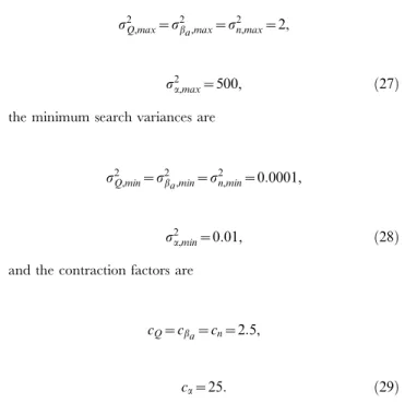
the maximum search variances for each parameter are
s2
Q,max~s2ba,max~s2n,max~2,
s2a,max~500, ð27Þ
the minimum search variances are
s2Q,min~s2b a,min~s
2
n,min~0:0001,
s2a,min~0:01, ð28Þ
and the contraction factors are
cQ~cba~cn~2:5,
ca~25: ð29Þ
The normalized quadratic error for each parameter qi,
i~1,. . .,4, is defined as,
Epi(n)~ð(pi{^qqi(n))=piÞ 2:
ð30Þ
Figure 3(A–D) shows the normalized quadratic errors for each parameter as a function of the number of iterations (nL). We can see how after 3|104 iterations all errors are very low for the
estimated parameters. The values of the normalized quadratic errors in the30,000-th iteration are:
EQ~2:7|10{8,Eba~8:7|10{7,
En~1:6|10{8,Ea~1:1|10{8: ð31Þ
Approximate Bayesian Computation
In Bayesian estimation theory the parameters are modeled as random variables, rather than unknown but deterministic num-bers. Consequently, ABC-based methods aim at approximating the probability distribution of the parameters, vectorq, conditional on the observations from the primary system. The technique, to be described next, is nonparametric, i.e., the distribution of q is approximated by a set of random samples.
ABC methods have been conceived with the aim of inferring posterior distributions without having to compute likelihood functions [35–39]. The calculation of the likelihood is replaced by a comparison between the observed and the simulated data. In the setup of this paper, the comparison is carried out between the data from the primary system (the observations) and the data generated by the secondary system (the model with adjustable parameters). The comparison between these data represents, in our case, a measure of the synchronization error between these two systems.
Letpdenote the a priori probability density function (pdf) of the random parameter vector q, let f(yDq) denote the probability distribution of the data y generated by the secondary system conditional on the realization of qand let d(x,y) be a distance function that measures the synchronization error by comparing the observed time series x from the primary system and the generated time seriesyfrom the secondary one. Since the system of interest is deterministic, f(yDq) collapses into a Dirac delta measure whenqis given. In the ABC framework, though, we are not interested in evaluatingf but rather in generatingyusing the model conditional onq. This amounts to integrating the secondary system with a given realization of the adjustable parametersq.
The simplest ABC algorithm is theABC rejection sampler[35]. For a given synchronization error threshold (often termed tolerance) w0, the algorithm can be described as follows.
Figure 3. Normalized quadratic errors for each parameter as a function of the number of iterations for the ARS algorithm.(A)Q, (B)
ba, (C )nand (D)a.
1. Sample~qqfromp(q).
2. Simulate a dataset ~yy from the conditional probability distributionf(yD~qq).
3. If the distance function (synchronization error) isd(x,~yy)ƒE, then accept~qq, otherwise reject it.
4. Return to the first step.
The output of an ABC algorithm is a population of parameter values randomly drawn from the distributionp(qDd(x,~yy)ƒ), i.e., a distribution with density proportional to the prior but restricted to the set of values ofqfor which the synchronization error is at most .
The disadvantage of the ABC rejection sampler is that the acceptance rate is very low when the set of values ofqfor which the synchronization error is less than turns out to be relatively small. Thus, instead of implementing this method we have decided to implement two more sophisticated ABC algorithms. The first one is a Markov chain Monte Carlo (ABC MCMC) technique and the second one is a sequential Monte Carlo (ABC SMC) method.
Approximate Bayesian Computation Markov Chain Monte Carlo
The Approximate Bayesian Computation Markov Chain Monte Carlo (ABC MCMC) algorithm is a Metropolis-Hastings [37] MCMC method that incorporates one additional test to ensure that all parameters in the chain yield a synchronization error below the threshold . It can be outlined as follows.
1. Initializeq(i),i~0.
2. Generate~qqaccording to a proposal distributiong(qDq(i))
3. Simulate a dataset ~yy from the conditional probability distributionf(yD~qq).
4. If the distance function (synchronization error) isd(x,~yy)ƒE, go to the following step, otherwise setq(iz1)~q(i)and go to step 6.
5. Setq(iz1)~~qqwith probability
j~min 1, p(~qq)g(q(i)D~qq) p(q(i))g(~qqDq(i))
ð32Þ
andq(iz1)~q(i)with probability1{j.
1. Seti~iz1, go to step 2.
The outcome of this algorithm is a Markov chain with the stationary distribution p(qDd(x,~yy)ƒE) [37]. The parameters are assumed independent a priori, hence
p(q)~ P
j~1,:::,mp(qi), ð33Þ
and we also choose independent proposals for simplicity. In particular, the prior distributions for each parameter have been chosen as
p(Q)~p(ba)~p(n)~U(0,5)
p(a)~U(0,500), ð34Þ
and the proposal distribution for each parameter is a Gaussian distribution centered at the previous value of the corresponding parameter and with a fixed standard deviation, different for each parameter. In particular,
s(Q)~s(ba)~s(n)~1
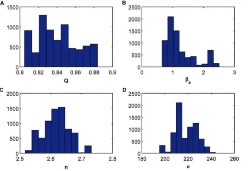
Figure 4. Histograms of the approximate marginal posterior distributions for each parameter for the ABC MCMC algorithm when consideringE~0:001.(A)Q, (B)ba, (C )nand (D)a.
s(a)~100 ð35Þ
and
g(qD~qq)~ P m
j~1N(qjDq
0
j,s(qj)): ð36Þ
Since the proposal distribution is symmetric,g(qiD~qq)~g(~qqDqi), and the prior is uniform, the acceptance probability in Eq.(32) isj~1. The distance function (synchronization error) has been chosen as
d(y,x)~ 1 To
ðTo
0
a a1{a1
j j2zjaa2{a2j2
dt
&1 N
X N{1 n~0
a
a1(nTs){a1(nTs)
ð Þ2zðaa2(nTs){a2(nTs)Þ2
ð37Þ
whereTo~105t.u. andNTs~T0. This expression is equivalent to
the cost function in the ARS method. The tolerance (threshold for the synchronization error) has been chosen asE~0:001.
A chain of5|105 samples has been generated, what implies
that the secondary system has been integrated5|105times. The
initial point of the chain is selected to ensure that the associated distance is less than0:05. Figure 4(A–D) shows the histograms of the approximate marginal posterior distributions for each param-eter. In order to reduce the strong correlation between consecutive samples in the Markov chain we have subsampled by a factor of 50. We have calculated the mean values of each histogram as well as the normalized quadratic errors according to the following expression
Epi~ð(pi{qqi)=piÞ2, ð38Þ
where qqi, for i~1,. . .,4, represents the mean value of the histogram of the corresponding parameter. The values of the normalized quadratic errors for the estimated parameters are
EQ~1:3|10{4,Eb
a~1:9|10 {1,
En~5:9|10{5,Ea~5:7|10{5: ð39Þ
We can see how three parameters are accurately estimated whereas for one of them, ba the error is significantly higher compared to (31).
Approximate Bayesian Computation Sequential Monte Carlo
A more sophisticated application of the ABC methodology is the Approximate Bayesian Computation Sequential Monte Carlo algorithm [39,54,55]. In ABC SMC, a number of sampled parameter values (often termed particles),fq(1),. . .,q(N)g, drawn
from the prior distribution p(q), are propagated through a sequence of intermediate distributions p(qDd(x,~yy)ƒi),
i~1,. . .,T{1, until they are converted into samples from the target distribution p(qDd(x,~yy)ƒT). The tolerances are chosen such
that 1w. . .wTw0, thus the empirical distributions gradually
evolve towards the target posterior. The ABC SMC algorithm proceeds as follows [39].
1. InitializeE1w. . .wET. Set the population indicatort~0. 2. Set the particle indicatori~1.
3. Ift~0, drawq?from the priorp(q).
Else, drawq?from
gt(q)~X N
i~1
w(i)(t{1)Kt(qDq(i)(t{1)) ð40Þ
where Kt(:Dq’) is a symmetric kernel centred around q’ and
w(1)(t{1),. . .,w(N)(t{1) are importance weights such that PN
i~1w(i)(t{1)~1.
4. Ifp(q?)~0, return to step 3.
5. Simulate a candidate dataset~yy~ff(yDq?).
6. Ifd(x,~yy)§Etreturn to step 3.
7. Setq(i)(t)~q?and calculate the weight,
wð Þti~
1,if t~0
p qð Þti
P N j~1w
(j)(t{1)Ktðq(i)(t{1)),q(j)(t)Þ tw0 8 > > > > < > > > > :
ð41Þ
8. IfivN, seti~iz1and go to step 3. 9. Normalize the weights.
10. IftvT, sett~tz1and go to step 2. Otherwise stop.
The prior distributions we have considered for each parameter arep(Q)~p(ba)~p(n)~U(0,5)and p(a)~U(0,500), the same
as for the ABC MCMC algorithm. The perturbation kernelKtis Gaussian, namely
Kt(q?Dq(i)(t{1))~P m
j~1N(q ? jDq
(i)
j (t{1),s(qj)), ð42Þ
with standard deviationss(Q)~s(ba)~s(n)~0:1ands(a)~10.
The distance function (synchronization error) is the same as for the
ABC MCMC and ARS algorithms with the sameTo value. To
ensure the gradual transition between populations, the ABC SMC algorithm is run for T~12 populations with ~f1,0:5,0:1,0:05, 0:025,0:01,0:005,0:0025,0:001,0:0005,0:00025,0:0001g and we have consideredN~400particles per population.
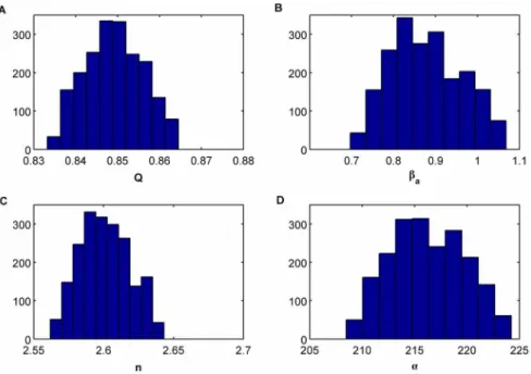
EQ~5:1|10{7,Eb
a~9:4|10 {4,
En~2:5|10{7,Ea~3:2|10{7: ð43Þ
Figure 6(A–D) shows the output (i.e. the accepted particles) of the ABC SMC algorithm as scatterplots of some of the two-dimensional parameter combinations, where we have information of different populations in the same plot. As we iterate the algorithm we obtain populations that are more dense around the desired values, as shown in these plots, where the particles from the prior are represented in blue, particles from population 2 in green, particles from population 4 in light blue, population 6 in
Figure 5. Histograms of the approximate marginal posterior distributions for each parameter for the ABC SMC algorithm when consideringE~0:0001.(A)Q, (B)ba, (C )nand (D)a.
doi:10.1371/journal.pone.0079892.g005
Figure 6. Two-dimensional scatterplots for the accepted particles of the ABC SMC of each population.The particles from the prior are represented in blue, particles from population 2 in green, particles from population 4 in cyan, population 6 in pink, 8 in yellow, 10 in red and particles from the posterior (population 12) in black color.
pink, 8 in yellow, 10 in red and particles from the posterior (population 12) in black color. We can see how for the last population the particles are tightly clustered around the desired value.
In order to gain insight of how the parameters are estimated during the evolution of the algorithm, we have represented some box–plot diagrams, one for each parameter to be estimated, as seen in fig. 7(A–D). In each diagram, we have information about the corresponding parameter as a function of the population index. In particular, the central mark of each box is the median of the population, the edges of the box are the 25-th and 75-th percentiles, the whiskers extend to the most extreme data points not considered as outliers, and the outliers are plotted individually using the plus symbols in red. The horizontal lines in red represent the actual values of the parameters we have used in our simulation. We can see from these plots how for a high enough population index the median values of the four parameters perfectly match the actual values.
We have also studied the computational cost of the algorithm. In fig. 8 we can see the number of samples or particles we have generated in order to have N~400 accepted particles for each population. We can see how the number of particles increases with the population index, being significantly high for the last population index, since it corresponds to a very small value of the synchronization error. Notice that the vertical axis of this figure is in a logarithmic scale.
Comparison of the Methods
Here we compare not only the accuracy but also the computational complexity of all three Monte Carlo methods for the joint estimation of the four parameters,Q,ba, n anda, of the chaotic intercellular network. To do that, we have calculated for the ABC SMC algorithm the computational load up to each population. Specifically, the computational complexity of gener-ating a sequence of m populations is given by the number of samples or particles that have to be generated before completing them{thpopulation. Note that the computational load for the
m{thpopulation also includes all samples needed to generate the
m{1previous populations.
Fig. 9 provides a graphical depiction of the complexity of the three methods, that we have investigated (ARS, ABC MCMC and ABC SMC algorithms). The line in red represents the complexity for the ARS method and the line in blue indicates the complexity for the ABC MCMC technique.
The parameter estimation errors attained with the ARS method are of the same order as the errors of the parameter estimates
computed from the 12{th population of the ABC SMC
algorithm. However, the number of samples generated to run the ARS procedure is&3|104while the ABC SMC technique
demands the generation of&4|105random samples up to the
12{th population. The ABC MCMC method achieves the
poorest performance, as it requires the generation of the highest number of samples (&5|105) and produces the largest errors (up
to three orders of magnitude worse than the ARS or ABC SMC estimates).
Figure 7. Box plots diagrams for the different populations for each parameter.(A) Q, (B)ba, (C ) n and (D)a.
doi:10.1371/journal.pone.0079892.g007
Figure 8. Computational cost for each population using the ABC SMC algorithm.
doi:10.1371/journal.pone.0079892.g008
Figure 9. Computational complexity measured by the number of random samples generated by the algorithms.The solid blue line is the complexity of the ABC MCMC algorithm (with~0:001). The solid red line is the complexity of the ARS method. The black dots indicate the complexity of the ABC SMC algorithm, for each population up to the12{thone.
Discussion
We have investigated three computational inference techniques for parameter estimation in a chaotic intercellular network that consists of two coupled modified repressilators. The proposed methodology combines a synchronization–based framework for parameter estimation in coupled chaotic systems with some state– of–the–art computational inference methods borrowed from computational statistics. In particular, we have focussed on an accelerated random search algorithm and two approximate Bayesian computation schemes (ABC MCMC and ABC SMC). The three methods exploit the synchronization property of chaotic systems. Therefore, it is not necessary to estimate the initial conditions of the variables, which is an important advantage from a computational point of view.
We have carried out the numerical study in this paper assuming that only two variables from the primary system can be observed. This is the minimum number of observed variables in order to guarantee the synchronization of the secondary system. If additional variables can be observed it is possible to easily incorporate them into the proposal methodology. For example, if the variablesx1,. . .,x8are observed (this is the full state of the first repressilator and the first variable,x8, of the second repressilator) we can redefine the distance function of Eq. (38) as
d(y,x)&1 N
X N{1 n~0
X8 i~1
xi(nTs){yi(nTs)
ð Þ2: ð44Þ
It can be verified (numerically) that using the distance in (44) (which intuitively provides ‘‘more information’’ about the primary system) leads to more accurate parameter estimates (or, alterna-tively, a greater number of parameters can be estimated if necessary). Note, however, that this comes at the expense of an additional computational effort and, moreover, it is unclear that all these variables can be accurately measured in practice.
The proposed methods can be applied when the observed time series are contaminated with additive noise of moderate variance. For example, if the observations have the form
~
a
a1(nTs)~a1(nTs)zu1(n)and~aa2(nTs)~a2(nTs)zu2(n),where
u1(n) and u2(n) are sequences of independent and identically distributed Gaussian noise variables with zero mean and variance
s2
u, then the distance function of Eq. (30) is lower-bounded by the
noise variance. Specifically, if^qq&pand, hence, we assume that
a
ai(nTs)&ai(nTs), it turns out that the distance d(y,x) is an estimator of (twice) the noise variance
d(y,x)
&1 N
X N{1 n~0
(aa1(nTs){~aa1(nTs))2z(aa2(nTs){~aa2(nTs))2
&2s2 u:
ð45Þ
This indicates that the synchronization error cannot go below the (approximate) bound of2s2
u and, therefore, the ABC-based
methods can work as long as the tolerances (t,t~1,. . .,T, in the
ABC SMC method, or E in the ABC MCMC technique) are
chosen to be greater than2s2
u. This means that the ABC SMC
algorithm withT~12populations andT~10{4can still provide
accurate parameter estimates when the observation noise variance iss2
uvT=2. In order to handle larger noise variances, one needs to
relax the coupling (i.e., choose a smaller coupling factorD) and increase the observation period To. This makes the distance function more sensitive to the discrepancy betweenqandp, which in practice means that we can choose a larger tolerance (e.g,T in
the ABC SMC algorithm) and preserve the accuracy of the resulting estimate^qq.
Author Contributions
Conceived and designed the experiments: IPM AZ. Performed the experiments: IPM. Analyzed the data: IPM EU AZ. Contributed reagents/materials/analysis tools: IPM EU AZ. Wrote the paper: IPM EU AZ.
References
1. van Vreeswijk C, Sompolinsky H (1996) Chaos in Neuronal Networks with Balanced Excitatory and Inhibitory Activity. Science 274: 1724–1726. 2. Amit DJ, Brunel N (1997) Model of global spontaneous activity and local
structured activity during delay periods in the cerebral cortex. Cereb. Cortex 7: 237–252.
3. Brunel N (2000) Dynamics of networks of randomly connected excitatory and inhibitory spiking neurons. J. Physiol Paris 94: 445–463.
4. Sompolinsky H, Crisanti A, Sommers HJ (1988) Chaos in random neural networks. Phys. Rev. Lett. 61: 259–262.
5. Sussillo D, Abbott LF (2009) Generating Coherent Patterns of Activity from Chaotic Neural Networks. Neuron 63: 544–557.
6. Ghosh A, Kumar VR, Kulkarni BD (2001) Parameter estimation in spatially extended systems: The Karhunen-Leve and Galerkin multiple shooting approach. Phys. Rev. E 64: 056222.
7. Baake E, Baake M, Bock HG, Briggs KM (1992) Fitting ordinary differential equations to chaotic data. Phys. Rev. A 45: 5524–5529.
8. Hatz K, Schloder JP, Bock HG (2012) Estimating Parameters in Optimal Control Problems. SIAM J. Sci. Comput. 34: A1707–A1728.
9. Petridis V, Paterakis E, Kehagias A (1998) A hybrid neural-genetic multimodel parameter estimation algorithm. IEEE Trans. Neural Networks 9: 862–876. 10. Timmer J (2000) Parameter estimation in nonlinear stochastic differential
equations. Chaos Solitons and Fractals 11: 2571–2578.
11. Singer H (2002) Parameter Estimation of Nonlinear Stochastic Differential Equations: Simulated Maximum Likelihood versus Extended Kalman Filter and It-Taylor Expansion. Journal of Computational and Graphical Statistics 11: 972–995.
12. Sitz A, Schwarz U, Kurths J, Voss HU (2002) Estimation of parameters and unobserved components for nonlinear systems from noisy time series. Phys Rev. E 66: 016210.
13. Pisarenko VF, SornetteD (2004) Statistical methods of parameter estimation for deterministically chaotic time series. Phys. Rev. E 69: 036122.
14. Parlitz U, Junge L, Kocarev L (1996) Synchronization-based parameter estimation from time series. Phys. Rev. E 54: 6253–6259.
15. Parlitz U (1996) Estimating Model Parameters from Time Series by Autosynchronization. Phys. Rev. Lett. 76: 1232–1235.
16. Zhou C, Lai C-H (1999) Decoding information by following parameter modulation with parameter adaptive control. Phys. Rev. E 59: 6629–6636. 17. Maybhate A, Amritkar RE (1999) Use of synchronization and adaptive control
in parameter estimation from a time series. Phys. Rev. E 59: 284–293. 18. d’Anjou A, Sarasola C, Torrealdea FJ, Orduna R, Grana M (2001)
Parameter-adaptive identical synchronization disclosing Lorenz chaotic masking. Phys. Rev. E 63: 046213.
19. Konnur R (2003) Synchronization-based approach for estimating all model parameters of chaotic systems. Phys. Rev. E 67: 027204.
20. Huang D (2004) Synchronization-based estimation of all parameters of chaotic systems from time series. Phys. Rev. E 69: 067201.
21. Freitas US, Macau EEN, Grebogi C (2005) Using geometric control and chaotic synchronization to estimate an unknown model parameter. Phys. Rev. E 71: 047203.
23. Marin˜o IP, Mı´guez J (2006) An approximate gradient-descent method for joint parameter estimation and synchronization of coupled chaotic systems. Phys. Lett. A 351: 262–267.
24. Tao C, Zhang Y, Jiang JJ (2007) Estimating system parameters from chaotic time series with synchronization optimized by a genetic algorithm. Phys. Rev. E 76: 016209.
25. Yang X, Xu W, Sun Z (2007) Estimating model parameters in nonautonomous chaotic systems using synchronization. Phys. Lett. A 364: 378–388. 26. Yu D, Parlitz U (2008) Estimating parameters by autosynchronization with
dynamics restrictions. Phys. Rev. E 77: 066221.
27. Ghosh D, Banerjee S (2008) Adaptive scheme for synchronization-based multiparameter estimation from a single chaotic time series and its applications. Phys. Rev. E 78: 056211.
28. Abarbanel HDI, Creveling DR, Farsian R, Kostuk M (2009) Dynamical State and Parameter Estimation. SIAM J. Appl. Dyn. Syst. 8: 1341–1381. 29. Sakaguchi H (2002) Parameter evaluation from time sequences using chaos
synchronization. Phys. Rev. E 65: 027201.
30. Schumann-Bischoff J, Luther S, Parlitz U (2013) Nonlinear system identification employing automatic differentiation. Commun. Nonlinear Sci. Numer. Simulat. 18: 2733–2742.
31. Marin˜o IP, Mı´guez J (2007) Monte Carlo method for multiparameter estimation in coupled chaotic systems. Phys. Rev. E 76: 057203.
32. van Leeuwen PJ (2010) Nonlinear data assimilation in geosciences: an extremely efficient particle filter. Q.J.R. Meteorol. Soc 136: 1991–1999.
33. Marin˜o IP, Mı´guez J, Meucci R (2009) Monte Carlo method for adaptively estimating the unknown parameters and the dynamic state of chaotic systems. Phys. Rev. E 79: 056218.
34. Appel MJ, Labarre R, Radulovic D (2003) On Accelerated Random Search. SIAM J. Optim. 14: 708–731.
35. Pritchard J, Seielstad MT, Perez-Lezaun A, Feldman MW (1999) Population growth of human Y chromosomes: a study of Y chromosome microsatellites. Mol. Biol. Evol. 16: 1791–1798.
36. Beaumont MA, Zhang W, Balding DJ (2002) Approximate Bayesian Computation in Population Genetics. Genetics 162: 2025–2035.
37. Marjoram P, Molitor J, Plagnol V, Tavare S (2003) Markov chain Monte Carlo without likelihood. Proc. Natl. Acad. Sci. U.S.A. 100: 15324–15328. 38. Sisson SA, Fan Y, Tanaka MM (2007) Sequential Monte Carlo without
likelihoods. Proc. Natl. Acad. Sci U.S.A. 104: 1760–1765.
39. Toni T, Welch D, Strelkowa N, Ipsen A, Stumpf MPH (2009) Approximate Bayesian computation scheme for parameter inference and model selection in dynamical systems. J. R. Soc. Interface 6: 187–202.
40. Elowitz MB, Leibler S (2000) A synthetic oscillatory network of transcriptional regulators. Nature 403: 335–338.
41. Ullner E, Koseka A, Kurths J, Volkov E, Kantz H, et al. (2008) Multistability of synthetic genetic networks with repressive cell-to-cell communication. Phys. Rev. E 78: 031904.
42. Garcı´a-Ojalvo J, Elowitz B, Strogatz SH (2004) Modeling a synthetic multicellular clock: Repressilators coupled by quorum sensing. Proc. Natl. Acad. Sci. U.S.A. 101: 10955–10960.
43. McMillen D, Kopell N, Hasty J, Collins JJ (2002) Synchronizing genetic relaxation oscillators by intercell signaling. Proc. Natl. Acad. Sci. U.S.A. 99: 679–684.
44. You L, Cox III RS, Weiss R, Arnold FH (2004) Programmed population control by cellcell communication and regulated killing. Nature 428: 868–871. 45. Volkov EI, Stolyarov MN (1991) Birhythmicity in a system of two coupled
identical oscillators. Phys. Lett. A 159, 61–66.
46. Han SK, Kurrer C, Kuramoto Y (1995) Dephasing and Bursting in Coupled Neural Oscillators. Phys. Rev. Lett. 75: 3190–3193.
47. Bala´zsi G, Cornell-Bell A, Neiman AB, Moss F (2001) Synchronization of hyperexcitable systems with phase-repulsive coupling. Phys. Rev. E 64: 041912. 48. Ullner E, Zaikin A, Volkov EI, Garcı´a-Ojalvo J (2007) Multistability and Clustering in a Population of Synthetic Genetic Oscillators via Phase-Repulsive Cell-to-Cell Communication. Phys. Rev. Lett. 99: 148103.
49. Koseka A, Ullner E, Volkov E, Kurths J, Garcı´a-Ojalvo J (2010), J. Theor. Biol. 263, 189.
50. Laje R, Mindlin GB (2002)., Phys. Rev. Lett. 89, 288102.
51. Koseska A, Volkov E, Zaikin A, Kurths J (2007) Inherent multistability in arrays of autoinducer coupled genetic oscillators. Phys. Rev. E 75: 031916. 52. Glass L, Mackey MC (1988) From Clocks to Chaos: The Rhythms of Life:
Princeton University Press, Princeton, NJ. 248p.
53. Meinhardt H (1982) Models of Biological Pattern Formation: Academic Press, New York.
54. Del Moral P, Doucet A, Jasra A (2006) Sequential Monte Carlo samplers. J. R. Stat. Soc B 68: 411–436.