DREAM<sub>(D)</sub>: an adaptive markov chain monte carlo simulation algorithm to solve discrete, noncontinuous, posterior parameter estimation problems

(1)

HESSD

8, 4025–4052, 2011

DREAM_(D)_→discrete MCMC simulation

J. A. Vrugt

Title Page

Abstract Introduction

Conclusions References

Tables Figures

◭ ◮

Back Close

Full Screen / Esc

Printer-friendly Version Interactive Discussion

Discussion

P

a

per

|

Dis

cussion

P

a

per

|

Discussion

P

a

per

|

Discussio

n

P

a

per

Hydrol. Earth Syst. Sci. Discuss., 8, 4025–4052, 2011 www.hydrol-earth-syst-sci-discuss.net/8/4025/2011/ doi:10.5194/hessd-8-4025-2011

Hydrology and Earth System Sciences Discussions

This discussion paper is/has been under review for the journal Hydrology and Earth System Sciences (HESS). Please refer to the corresponding final paper in HESS if available.

DREAM

₍

_D

₎

: an adaptive markov chain

monte carlo simulation algorithm to solve

discrete, noncontinuous, posterior

parameter estimation problems

J. A. Vrugt1,2

1

Department of Civil and Environmental Engineering, University of California, Irvine, 4130 Engineering Gateway, Irvine, CA 92697-2175, USA

2

Institute for Biodiversity and Ecosystem Dynamics, University of Amsterdam, Amsterdam, The Netherlands

Received: 19 April 2011 – Accepted: 20 April 2011 – Published: 26 April 2011 Correspondence to: J. A. Vrugt (jasper@uci.edu)

(2)

HESSD

8, 4025–4052, 2011

J. A. Vrugt

Title Page

Tables Figures

◭ ◮

Back Close

Full Screen / Esc

Discussion

P

a

per

|

Dis

cussion

P

a

per

|

Discussion

P

a

per

|

Discussio

n

P

a

per

|

Abstract

Formal and informal Bayesian approaches are increasingly being used to treat forcing, model structural, parameter and calibration data uncertainty, and summarize hydro-logic prediction uncertainty. This requires posterior sampling methods that approxi-mate the (evolving) posterior distribution. We recently introduced the DiffeRential Evo-5

lution Adaptive Metropolis (DREAM) algorithm, an adaptive Markov Chain Monte Carlo (MCMC) method that is especially designed to solve complex, high-dimensional and multimodal posterior probability density functions. The method runs multiple chains in parallel, and maintains detailed balance and ergodicity. Here, I present the latest algorithmic developments, and introduce a discrete sampling variant of DREAM that 10

samples the parameter space at fixed points. The development of this new code, DREAM(D), has been inspired by the existing class of integer optimization problems,

and emerging class of experimental design problems. Such non-continuous parameter estimation problems are of considerable theoretical and practical interest. The theory developed herein is applicable to DREAM(ZS) (Vrugt et al., 2011) and MT-DREAM(ZS)

15

(Laloy and Vrugt, 2011) as well. Two case studies involving a sudoku puzzle and rainfall – runo_ffmodel calibration problem are used to illustrate DREAM_(D).

1 Introduction

Formal and informal Bayesian methods have found widespread application and use to summarize parameter and model predictive uncertainty in hydrologic modeling. These 20

parameters generally represent model dynamics, but could also include rainfall multipli-ers (Kavetski et al., 2006; Kuczera et al., 2006; Vrugt et al., 2008), error model variables (Smith et al., 2008; Schoups and Vrugt, 2010), and calibration data measurement er-rors (Sorooshian and Dracup, 1980; Schaefli et al., 2007; Vrugt et al., 2008). Monte Carlo methods are admirably suited to generate samples from the posterior param-25

(3)

HESSD

8, 4025–4052, 2011

J. A. Vrugt

Title Page

Tables Figures

◭ ◮

Back Close

Full Screen / Esc

Discussion

P

a

per

|

Dis

cussion

P

a

per

|

Discussion

P

a

per

|

Discussio

n

P

a

per

and high-dimensional model-data synthesis problems. This has stimulated the devel-opment of Markov Chain Monte Carlo (MCMC) methods that generate a random walk through the search (parameter space) and iteratively visit solutions with stable frequen-cies stemming from an invariant probability distribution. If well designed, such MCMC methods should be more efficient than brute force Monte Carlo or importance sampling 5

methods.

To visit configurations with a stable frequency, an MCMC algorithm generates trial moves from the current position of the Markov chainx_t₋₁to a new statez. The earliest and most general MCMC approach is the random walk Metropolis (RWM) algorithm (Metropolis et al., 1953). Assume that we have already sampled points_{x₀,...,x_t₋₁_} 10

this algorithms proceeds in the following three steps. First, a candidate point z is sampled from a proposal distributionqthat depends on the present location,x_t₋₁and is symmetric, q(x_t₋1,z)=q(z,xt−1). Next, the candidate point is either accepted or

rejected using the Metropolis acceptance probability:

α(x_t₋₁,z)₌

(

min_π₍π_x(z)

t−1),1

ifπ(x_t₋₁)>0

1 ifπ(x_t₋₁)₌0 (1)

15

whereπ(·) denotes the probability density function (pdf) of the target distribution. Fi-nally, if the proposal is accepted the chain moves to z, otherwise the chain remains at its current locationx_t₋₁. The result is a Markov chain which under some regularity conditions has a unique stationary distribution with pdfπ(·).

The standard RWM algorithm has been designed to maintain detailed balance with 20

respect toπ(_·) at each step in the chain:

π(x_t₋₁)p(x_t₋₁_→z)₌π(z)p(z_→x_t₋₁) (2)

whereπ(xt₋1) (π(z)) denotes the probability of finding the system in statext₋1(z), and

p(x_t₋1→z)(p(z→xt−1)) denotes the conditional probability to perform a trial move

(4)

HESSD

8, 4025–4052, 2011

J. A. Vrugt

Title Page

Tables Figures

◭ ◮

Back Close

Full Screen / Esc

Discussion

P

a

per

|

Dis

cussion

P

a

per

|

Discussion

P

a

per

|

Discussio

n

P

a

per

|

toz and the reverse jump do not have equal probability. This extension is called the Metropolis Hastings algorithm (MH), and has become the basic building block of many existing MCMC sampling schemes.

Existing theory and experiments prove convergence of well-constructed MCMC schemes to the appropriate limiting distribution under a variety of different conditions. 5

In practice, this convergence is often observed to be impractically slow. This deficiency is frequently caused by an inappropriate selection ofq(_·) used to generate trial moves in the Markov Chain. This inspired Vrugt et al. (2008, 2009) to develop a simple adap-tive RWM algorithm called Differential Evolution Adaptive Metropolis (DREAM) that runs multiple chains simultaneously for global exploration, and automatically tunes the 10

scale and orientation of the proposal distribution during the evolution to the posterior distribution. This scheme is an adaptation of the Shuffled Complex Evolution Metropolis (Vrugt et al., 2003) global optimization algorithm and has the advantage of maintaining detailed balance and ergodicity while showing excellent efficiency on complex, highly nonlinear, and multimodal target distributions (Vrugt et al., 2008, 2009).

15

In DREAM,N different Markov Chains are run simultaneously in parallel. If the state of a single chain is given by a singled-dimensional vectorx, then at each generation theN chains in DREAM define a populationX, which corresponds to anN xd matrix, with each chain as a row. Jumps in each chaini={1,...,N_}are generated by taking a fixed multiple of the difference of the states of randomly chosen pairs of chains ofX: 20

zi=xi+(1_d+e_d)γ(δ,d′)





δ

X

j=1

xr1(j)₋ δ

X

n=1

xr2(n)



+ǫ_d (3)

whereδ signifies the number of pairs used to generate the proposal, xr1(j) _and _xr2(n) are randomly selected without replacement from the population X−_ti

−1 (the population

withoutxi_t₋₁); r1(j),r2(n)∈ {1,...,N}and r1(j)6=r2(n). The values ofed and ǫd are drawn fromU_d(₋b,b) and N_d(0,b∗) withb and b∗ small compared to the width of the 25

(5)

HESSD

8, 4025–4052, 2011

J. A. Vrugt

Title Page

Tables Figures

◭ ◮

Back Close

Full Screen / Esc

Discussion

P

a

per

|

Dis

cussion

P

a

per

|

Discussion

P

a

per

|

Discussio

n

P

a

per

d′, the number of dimensions that will be updated jointly. By comparison with RWM, a good choice forγ=2.4/√2δd′_{(Roberts and Rosenthal, 2001; Ter Braak, 2006). This}

choice is expected, for Gaussian and Student target distributions, to yield an accep-tance probability of 0.44 ford′ =1, 0.28 for d′ = 5 and 0.23 for large d′. Every 5th generationγ=1.0 to facilitate jumping between disconnected posterior modes (Vrugt 5

et al., 2008).

The difference vector in Eq. (3) contains the desired information about the scale and orientation of the target distribution,π(x_|·). By accepting each jump with the Metropo-lis ratio minnπ(zi_|·)/π(xi_t₋₁_|·),1o, a Markov chain is obtained, the stationary or limiting distribution of which is the posterior distribution. The proof of this is given in Ter Braak 10

and Vrugt (2008) and Vrugt et al. (2008, 2009). Because the joint pdf of theN chains factorizes toπ(x1_|·)_×..._×π(xN_|·), the statesx1...xN of the individual chains are inde-pendent at any generation after DREAM has become indeinde-pendent of its initial value. After this burn-in period, the convergence of DREAM can thus be monitored with the

ˆ

R-statistic of Gelman and Rubin (1992). This convergence diagnostic compares the 15

within and in-between variances of theN di_fferent chains.

Various recent contributions have shown the utility of MCMC simulation with DREAM to treat different error sources, and help quantify and analyze parameter, model struc-tural, forcing, and calibration data uncertainty (Vrugt et al., 2008, 2009b; Dekker et al., 2010; He et al., 2010; Huisman et al., 2010; Keating et al., 2010; Minasny et al., 20

2011; Schoups and Vrugt, 2010; Vrugt et al., 2011). These, and most other model-data synthesis studies in the earth sciences, typically involve continuous variables (parame-ters and probability density functions) that can take on any numerical value within their prior ranges defined by the user. Yet, relatively little attention has been given to pos-terior sampling problems involving discrete variables. The existing DREAM framework 25

has been developed based on the assumption of continuity of the parameter space, lim

(6)

HESSD

8, 4025–4052, 2011

J. A. Vrugt

Title Page

Tables Figures

◭ ◮

Back Close

Full Screen / Esc

Discussion

P

a

per

|

Dis

cussion

P

a

per

|

Discussion

P

a

per

|

Discussio

n

P

a

per

|

in many fields of study, and therefore of considerable theoretical and practical inter-est. For instance, in hydrology there is increasing interest in using optimization ap-proaches to help find optimal experimental design strategies that attempt to minimize cost, parameter and model predictive uncertainty, or combinations thereof. This in-volves selecting one or multiple di_fferent measurement locations amongst a discrete 5

set of possibilities. The solution of this problem lies in an adaptation of DREAM, and its various extensions including DREAM(ZS) (Vrugt et al., 2011), and MT-DREAM(ZS)

(Laloy and Vrugt, 2011).

In this paper we present a discrete implementation of DREAM, that is especially designed to solve noncontinuous search and optimization problems. This new code, 10

DREAM_(D)uses DREAM as its main building block, yet implements integer search to facilitate solving discrete sampling problems. The DREAM(D)algorithm maintains

de-tailed balance and ergodicity, and achieves excellent performance across a range of noncontinuous posterior sampling problems. The DREAM_(D)code is perhaps the only method available to solve discontinuous parameter estimation problems, and simulta-15

neously provide an estimate of uncertainty.

The remainder of this paper is organized as follows. Section 2 presents a short intro-duction to MCMC, followed by a detailed description of DREAM(D)in Sect. 3. Section 4

demonstrates the performance of DREAM(D)using two different case studies involving

a simple 52-dimensional sudoku puzzle, and a rainfall-runoffmodel calibration problem. 20

These results are illustrated in detail, and used to highlight further possible improve-ments. Finally, in Sect. 5 we summarize the methodology and discuss the results.

2 Nonlinear optimization involving discrete variables

Discrete optimization problems are abundant in many fields of study, and have begun to appear in the hydrologic literature (Furman et al., 2004; Harmancioglu et al., 2004; 25

(7)

HESSD

8, 4025–4052, 2011

J. A. Vrugt

Title Page

Tables Figures

◭ ◮

Back Close

Full Screen / Esc

Discussion

P

a

per

|

Dis

cussion

P

a

per

|

Discussion

P

a

per

|

Discussio

n

P

a

per

puzzle consisting of sixteen different surfaces. Each tile contains a different letter from the alphabet. The goal is to get the letters in the appropriate order. The solution to this problem is immediately obvious to a human, but not immediately clear to a computer. A search algorithm is therefore required to solve this problem.

If we assign numbers to each letter, a=1, b=2 and so forth, we could measure 5

the distance from our initial guess to the actual solution. This constitutes an integer optimization problem. The tiles can only take on integer values, between 1 and 16. This results in a d=16 dimensional search problem with each dimensionx∈[1,2,...,16]. Figure 1a illustrates an initial guess, and in a series of panels (B⇒D) it is shown how DREAM(D)translates this guess into the final solution.

10

Other problems that require integer search involve finding optimal experimental de-sign strategies. Usually this consists of finding the best measurement locations among a prior defined and often restricted set of possibilities. This requires integer optimiza-tion in a similar way as done in the tile puzzle.

3 DREAM_(D)_⇒di_fferential evolution adaptive metropolis with discrete sampling

15

We now describe our new code, entitled DREAM(D), which uses DREAM as main

build-ing block.

Let X be a N×d-matrix defining the N initialized starting positions, xi, i=1,...,N of the different Markov chains by drawing samples from p_d(x), the prior distribution. Similarly, letZbe an external archive of points that periodically appends the elements 20

ofX at regular intervals. The initial population [X_t;t=0] is translated into a sample from the posterior target distribution using the following pseudo code:

1. SetT←1

FORm←1,...,K DO (POPULATION EVOLUTION)

FORi_←1,...,NDO (CHAIN EVOLUTION)

(8)

HESSD

8, 4025–4052, 2011

J. A. Vrugt

Title Page

Tables Figures

◭ ◮

Back Close

Full Screen / Esc

Discussion

P

a

per

|

Dis

cussion

P

a

per

|

Discussion

P

a

per

|

Discussio

n

P

a

per

|

a. Generate a candidate point,zi in chaini,

zi₌xi₊

(1_d+e_d)γ(δ,d′)





δ

X

j=1

xr1(j)₋ δ

X

n=1

xr2(n)



+ǫ_d

d

(4)

where the function_{k · k}_d rounds each elementj=1,...,d of the jump vector to the nearest integer.

b. Replace each element (j=1,...,d) of the proposalzi_jwithzi_j using a binomial 5

scheme with probability 1−CR,

z_ji=

(

x_ji ifU_≤1₋CR, d′=d′−1

z_ji otherwise j=1,...,d (5)

whereCR denotes the crossover probability, andU ∈[0,1] is a draw from a uniform distribution.

c. Computeπ(zi) and accept the candidate points with Metropolis acceptance 10

probability,α(xi,zi),

α(xi,zi)=

(

min_ππ(₍z_xii)₎,1

ifπ(xi)>0

1 ifπ(xi)=0

(6)

d. If accepted, move the chain to the candidate point,xi₌zi, otherwise remain at the old location,xi.

15

END FOR (CHAIN EVOLUTION) END FOR (POPULATION EVOLUTION)

2. AppendX toZ.

(9)

HESSD

8, 4025–4052, 2011

J. A. Vrugt

Title Page

Tables Figures

◭ ◮

Back Close

Full Screen / Esc

Discussion

P

a

per

|

Dis

cussion

P

a

per

|

Discussion

P

a

per

|

Discussio

n

P

a

per

4. If ˆRj≤1.2 forj=1,...,d orT > Tmax, stop and go to step 5, otherwise setT←T+1

and go to POPULATION EVOLUTION.

5. Summarize the posterior pdf usingZ after discarding the initial and burn-in sam-ples.

The DREAM(D) algorithm presented herein is similar as DREAM, but especially

de-5

signed to solve discrete search and optimization problems. The function_⌈·⌋_d in Eq. (4) forces the jumps to maintain integer values, and maintains detailed balance (as demon-strated later). Compared to the original DREAM sampling scheme, DREAM(D)contains

two additional algorithmic parameters. These areTmax, the maximum number of

gen-erations, and K, the thinning rate used to periodically add samples to Z. Based on 10

recommendations in (Vrugt et al., 2011), we setK=10, and assign a large value for Tmax, thus DREAM(D) automatically stops after convergence has been achieved. To

speed up convergence to the target distribution, DREAM estimates a distribution of CR values during burn-in that favors large jumps over smaller ones in each of theN chains. Details of this can be found in (Vrugt et al., 2008, 2009, 2011).

15

The transition kernel in DREAM_(D) is especially designed to handle discrete search and optimization problems, yet only samples integer values. This is by no means a limitation, but a simple computational trick is therefore required to solve non-integer problems. For such problems, we discretize the range of each individual parameter into equidistant intervals, and rewrite the actual problem using integers only. The posterior 20

distribution of these integers is subsequently derived with DREAM(D). For example,

consider a discrete parameter that can only take on the values x1∈[0,0.2,0.4,...,5].

We can rewrite this problem as: x1=min(x1)+0.2j and samplej∈[0,1,...,25] using

DREAM(D). This approach, if deemed necessary, allows for a different discretization

of each individual parameter. Also, the simultaneous use of DREAM and DREAM_(D), 25

(10)

HESSD

8, 4025–4052, 2011

J. A. Vrugt

Title Page

Tables Figures

◭ ◮

Back Close

Full Screen / Esc

Discussion

P

a

per

|

Dis

cussion

P

a

per

|

Discussion

P

a

per

|

Discussio

n

P

a

per

|

3.1 DREAM(D)⇒Detailed Balance?

We are now left with a proof that DREAM(D)yields an invariant distribution that is

iden-tical to the posterior distribution. For this we need to demonstrate that the transition kernel in DREAM maintains detailed balance, and thus results in a reversible Markov chain. This essentially means that the forward (p(xi→zi)) and backward (p(zi→xi)) 5

jump have equal probability at every single step in the chain. This is easy to proof for standard RWM algorithms that use a fixed proposal distribution. Yet, the jumping distri-bution used in DREAM(D)is adaptive, and continuously changes scale and orientation

en route to the posterior distribution. This significantly enhances efficiency, but it is not immediately clear whether Eq. (4) also satisfies the detailed balance condition.

10

In previous papers, we have given formal proofs of convergence of DREAM (Vrugt et al., 2008), DREAM(ZS) (Vrugt et al., 2011), and MT-DREAM(ZS) (Laloy and Vrugt,

2011) to the appropriate limiting distribution. For simplicity, we use a hypothetical ex-ample to illustrate that DREAM(D) maintains detailed balance. Lets consider a

two-dimensional, (d=2) discrete sampling problem withN=5 different chains,δ=1, and 15

γ=2.4/√2δd′₌₂_.₄_/√₂_×₁_×₂₌₁_._{2. The initial states of these chains are color coded}

and depicted in Fig. 2, and used to generate candidate points. Lets assume that the jump in the first chain (purple) uses the states of the 2nd (r1: blue), and 4th (r2: green)

chain, and thatej=ǫj=0;j=1,...,2. Following Eq. (4), the forward jump and proposal point then becomes:

20

zi₌

2 2

+

1.2

4 4 −

5 1

=

2 2

+

−1.2 3.6

=

1 6

(7)

This point is indicated in Fig. 2 with the red square. Lets assume that we accept this candidate point, and chain 1 transitions to this new state.

We are now left with studying the probability of the backward jump. This requires the green chain to ber1, and the blue chain to ber2, thus selected in opposite order

25

(11)

HESSD

8, 4025–4052, 2011

J. A. Vrugt

Title Page

Tables Figures

◭ ◮

Back Close

Full Screen / Esc

Discussion

P

a

per

|

Dis

cussion

P

a

per

|

Discussion

P

a

per

|

Discussio

n

P

a

per

respective chain pairs for the candidate point. Hence, the chance to selectr1as chain

2, andr2as chain 4 is equal to drawingr2=4, andr2=2. Reversibility is thus ensured,

yet is is not directly obvious that this proof also holds for DREAM(D)that uses an explicit

integer rounding function in the transition kernel. If we proceed with our new selection ofr1andr2then the next candidate point becomes:

5

zi=

1 6

+ 1.2

5 1 −

4 4

=

1 6

+

1.2₋3.6

=

2 2

(8)

Indeed, the reverse jump results in a proposal point that is identical to the initial state of chain 1 (purple point), and reversibility is ensured. Apparently, the function,

k · kd, used to round thed-dimensional jumping vector to the closest integers does not violate detailed balance. This proof also holds whene_d, andǫd are drawn from their 10

respective symmetric probability distributions, and whenδ >1 andd >2. We leave this up to the reader. This concludes the proof of detailed balance.

A final remark is appropriate. In theory it is possible that at least one of thed argu-ments,y_d of the rounding function,_ky_d_khas a fractional part of.5. Or in mathematical notation,_∃y_j_∈Y_j:y_j_−ky_j_k=0.5;j=1,...,d, whereY_j denotes the feasible jump space 15

of thejth dimension, generated with Eqs. (3) or (4). If this (mathematical) statement is true, then the respective argument(s) is (are) rounded down (floor) to the closest in-teger. This directed rounding violates detailed balance and introduces a possible bias in the proposal jump. A simple one-dimensional example will immediately illustrate this, but the chance this bias happens in practice is virtually zero. If nothing else, the 20

stochastic nature ofe_d_∼U_d(₋b,b), andǫ_d_∼N_d(0,b∗) will eliminate this possibility. In the rare event ofyj− kyjk=0.5 we implement stochastic rounding, and choice among y_j−0.5 and y_j+0.5 with equal probability. This ensures reversibility of the Markov chains generated with DREAM(D). Note that the size ofYj essentially depends on the choice of the prior distribution.

(12)

HESSD

8, 4025–4052, 2011

J. A. Vrugt

Title Page

Tables Figures

◭ ◮

Back Close

Full Screen / Esc

Discussion

P

a

per

|

Dis

cussion

P

a

per

|

Discussion

P

a

per

|

Discussio

n

P

a

per

|

4 Case studies

I now present two different case studies with increasing complexity. The first study consists of a typical integer estimation problem, and involves a sudoku puzzle. This puzzle has become quite popular in the past 10 years, and many newspapers, jour-nals, and magazines around the world publish sudokus for entertainment. This syn-5

thetic study illustrates the ability of DREAM_(D)to help solve a relatively difficult integer optimization problem. The second study is concerned with estimating parameters in a mildly complex lumped watershed model using observed daily discharge data from the Guadalupe River in Texas. The parameter estimation problem is posed in discrete form, and solved using DREAM_(D). This results in a discrete The posterior parameter 10

distribution is compared against a classical continuous formulation of the model cali-bration inverse problem separately inferred using DREAM(ZS), and used to highlight the

advantages of DREAM_(D)and discrete sampling.

4.1 The daily sudoku

The first case study considers a synthetic integer parameter estimation problem, in-15

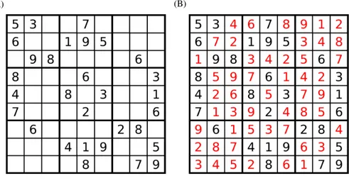
volving a sudoku puzzle. The objective is to fill a 9_×9 grid with digits so that each column, each row, and each of the nine 3_×3 sub-grids that make up the total square contains values of 1 to 9. The same single integer may not appear twice in the same 9_×9 playing board row or column or in any of the nine 3_×3 subregions. The puzzle setter provides a partially completed grid, which typically has a single (unique) solution. 20

The puzzle was popularized in 1986 by the Japanese puzzle company Nikoli, under the name Sudoku, meaning single number (Hayes, 2006). Nowadays, Sudoku puzzles are very popular, and widely practised by many millions of people throughout the world.

I consider the Sudoku puzzle in Fig. 3, taken from Wikipedia (http://en.wikipedia. org/wiki/Sudoku). The initial grid is depicted at the left-hand side, whereas the final 25

(13)

HESSD

8, 4025–4052, 2011

J. A. Vrugt

Title Page

Tables Figures

◭ ◮

Back Close

Full Screen / Esc

Discussion

P

a

per

|

Dis

cussion

P

a

per

|

Discussion

P

a

per

|

Discussio

n

P

a

per

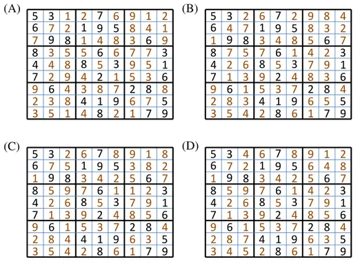
estimated. These parameters can take on values between 1 to 9. Figure 4 illustrates the sampled values of DREAM_(D)at various stages during the integer search. A total of N=25 different chains were used to search the parameter space, and the initial sample was created using Latin Hypercube Sampling. I did not impose any constraints on this initial solution, and thus each value of 1 to 9 can appear in any number in the 5

grid. The log-likelihood function measures the constraint violation, details of which are outside the scope of this publication.

The first grid, at the left-hand side of Fig. 4 presents an example of a possible starting solution used in one of the chains. Obviously, this solution is rather bad, and violates each of the three different constraints discussed previously (1 to 9 in each column 10

and row, and each 3_×3 subregion). The second grid, Fig. 4b, shows considerable improvements, and better resemblances the final solution. The third panel in Fig. 4c is a further refinement, but with a few noticeable deviations from the true solution. Finally, after about 1 million sudoku function evaluations, the puzzle is successfully solved (Fig. 4d).

15

Obviously, it is inspiring that DREAM(D)is able to successfully solve a Sudoku puzzle,

but the required number of function evaluations (computational time) to do so is rather large. Indeed, a branch and bound optimization approach would be about 3 orders of magnitude more efficient. Such an approach shuffles the d=52 integer values until all constraint are met. We could implement this procedure in DREAM(D), and

20

change the proposal distribution in such a way that jumps in each individual chain are no longer created by taking the difference of the states of two (or more) other chains but simply generated by shuffling selected parameter values of the same chain. Yet, it is not directly obvious how to make such modification and ensure reversibility of the Markov chain. This is an interesting problem, and deserves additional investigation, 25

(14)

HESSD

8, 4025–4052, 2011

J. A. Vrugt

Title Page

Tables Figures

◭ ◮

Back Close

Full Screen / Esc

Discussion

P

a

per

|

Dis

cussion

P

a

per

|

Discussion

P

a

per

|

Discussio

n

P

a

per

|

4.2 Watershed model calibration using discrete parameter estimation

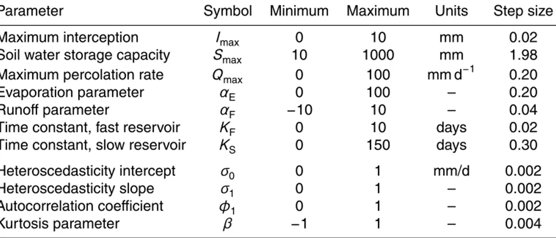
The final case study involves flood forecasting, and consists of the calibration of a mildly complex lumped watershed model using historical data from the Guadalupe River at Spring Branch, Texas. This is the driest of the 12 MOPEX basins described in the study of Duan et al. (2006). The model structure and hydrologic process representations are 5

found in (Schoups and Vrugt, 2010). The model transforms rainfall into runoffat the watershed outlet using explicit process descriptions of interception, throughfall, evap-oration, runoff generation, percolation, and surface and subsurface routing. Table 1 summarizes the seven different model parameters, and their prior uncertainty ranges. Each parameter is discretized equidistantly in 250 intervals with respective step size 10

listed in the last column at the right hand side. This gridding is necessary to create a non-continuous, discrete, parameter estimation problem. Unlike the previous case study in which integer values are sampled only, this particular study (mostly) involves non-integer values.

Daily discharge, mean areal precipitation, and mean areal potential evapotranspi-15

ration were derived from (Duan et al., 2006) and used for model calibration. Details about the basin, experimental data, and likelihood function can be found there, and will not be discussed herein. The same model and data was used in a previous study (Schoups and Vrugt, 2010), and used to introduce a generalized likelihood function for heteroscedastic, non-Gaussian, and correlated (streamflow) prediction errors.

20

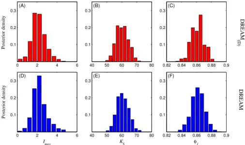
Figure 5 presents histograms of the marginal distribution of a selected few hydrologic model parameters using five years of observed daily discharge data. The top panel presents the results of DREAM_(D), whereas the bottom panel presents the results for a continuous parameter space. These histograms were derived by separately running DREAM for the same data set and model. Notice the close agreement between the 25

(15)

HESSD

8, 4025–4052, 2011

J. A. Vrugt

Title Page

Tables Figures

◭ ◮

Back Close

Full Screen / Esc

Discussion

P

a

per

|

Dis

cussion

P

a

per

|

Discussion

P

a

per

|

Discussio

n

P

a

per

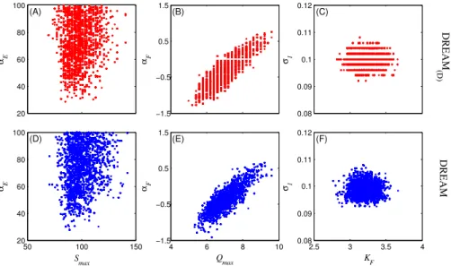
To better illustrate the effect of discretization, please consider Figure 6 that presents two-dimensional scatter plots of the DREAM_(D)derived posterior samples for a few se-lected parameter pairs. The bottom panel shows similar plots but then assuming conti-nuity of the parameter space. The effect of gridding is immediately apparent. Whereas the original bivariate scatter plots sample the parameter space in a (bloodstain) spatter 5

pattern, two-dimensional plots of the posterior samples derived with DREAM(D)exhibit

an obvious grid pattern with horizontally and vertically aligned points. The posterior samples take on discrete values with a distance between subsequent points that is similar to the intervals listed in Table 1. Despite this difference in sampling pattern, the shape of the DREAM and DREAM(D) derived bivariate scatter plots are very similar,

10

commensurate with the covariance structure of the posterior distribution. The results presented in Fig. 5 inspire confidence in the ability of DREAM(D)to solve

noncontinu-ous posterior sampling problems.

The excellent correspondence of the posterior parameter distributions derived with DREAM and DREAM(D)results in marginal differences of the resulting streamflow

pre-15

dictions. I therefore do not show any times series plots of model predictions, and cor-responding 95% uncertainty ranges. Such plots can be found in (Schoups and Vrugt, 2010) and details can be found in that publication. It is interesting to observe that the maximum log-likelihood value of 543 found with DREAM(D)is somewhat larger than its

counterpart estimated with DREAM (540). This difference was consistently observed 20

for multiple different trials with both MCMC algorithms.

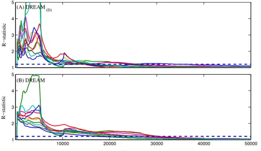
To provide better insights into the efficiency of DREAM(D), Fig. 7a plots the evolution

of the ˆR-statistic of Gelman and Rubin (Gelman and Rubin, 1992) for each of the different parameters. To benchmark these results, the bottom panel (Fig. 7b) illustrates the convergence results of DREAM assuming continuity of the parameter space. The 25

(16)

HESSD

8, 4025–4052, 2011

J. A. Vrugt

Title Page

Tables Figures

◭ ◮

Back Close

Full Screen / Esc

Discussion

P

a

per

|

Dis

cussion

P

a

per

|

Discussion

P

a

per

|

Discussio

n

P

a

per

|

feasible parameter space, this has no immediate effect on sampling efficiency. An approximately similar number of model runs is required to converge to and explore the posterior target distribution. Yet, this by no means is a universal finding. My initial results to date for more complex models with much higher parameter dimensionality demonstrate considerable enhancements in e_fficiency (sometimes dramatically) when 5

solving the calibration problem in the discretized rather than continuous space. Such transformation is particularly useful for insensitive parameters as gridding significantly reduces the space of feasible solutions. Further research on this topic is warranted.

5 Conclusions

In the past decade much progress has been made in the development of sampling 10

algorithms for statistical inference of the posterior parameter distribution. The typical assumption in this work is that the parameters are continuous and can take on any value within their upper and lower bounds. Unfortunately, such problems typically do not work for discrete parameter estimation problems. Such problems are abundant in many fields of study, and therefore of considerable theoretical and practical interest. 15

Examples include selecting among different measurement locations in the design of op-timal experimental strategies, finding the best members of an ensemble of predictors, and more generally discrete model calibration problems. Here, I have introduced a dis-crete MCMC simulation algorithm that is especially designed to solve non-continuous posterior sampling problems. This method, entitled DREAM(D) uses DREAM as its

20

main building block, yet uses a modified proposal distribution to facilitate solve discrete sampling problems. The DREAM_(D) algorithm maintains detailed balance and ergod-icity, and receives good performance across a range of problems involving a sudoku puzzle, and discrete rainfall – runoffmodel calibration problem.

The theory developed herein is easily implemented in DREAM(ZS)(Vrugt et al., 2011)

25

and MT-DREAM_(ZS)(Laloy and Vrugt, 2011), which provides a venue to further increase the efficiency of MCMC simulation. The DREAM(D)code is written in MATLAB and is

(17)

HESSD

8, 4025–4052, 2011

J. A. Vrugt

Title Page

Tables Figures

◭ ◮

Back Close

Full Screen / Esc

Discussion

P

a

per

|

Dis

cussion

P

a

per

|

Discussion

P

a

per

|

Discussio

n

P

a

per

Acknowledgements. I gratefully acknowledge the insightful comments of the three different re-viewers. Computer support, provided by the SARA center for parallel computing at the Univer-sity of Amsterdam, The Netherlands, is highly appreciated.

References

Box, G. E. P. and Tiao, G. C.: Bayesian Inference in Statistical Analyses

Addison-Wesley-5

Longman, Reading, Massachusetts, 1973.

Dekker, S. C., Vrugt, J. A., and Elkington, R. J.: Significant variation in vegetation charac-teristics and dynamics from ecohydrologic optimality of net carbon profit, Ecohydrology, doi:10.1002/eco.177, 2010. 4029

Duan, Q., Gupta, V. K., and Sorooshian, S.: Effective and efficient global optimization for

10

conceptual rainfall-runoffmodels, Water Resour. Res., 28, 1015–1031, 1992.

Duan, Q., Schaake, J., Andrassian, V., Franks, S., Goteti, G., Gupta, H. V., Gusev, Y. M., Habets, F., Hall, A., Hay, L., Hogue, T., Huang, M., Leavesley, G., Liang, X., Nasonova, O. N., Noilhan, J., Oudin, L., Sorooshian, S., Wagener, T., and Wood, E. F.: Model Parameter Estimation Experiment (MOPEX): An overview of science strategy and major results from

15

the second and third workshops, J. Hydrol., 320, 3–17, 2006. 4038

Furman, A., Ferr ´e, T. P. A., and Warrick, A. W.: Optimization of ERT surveys for monitoring transient hydrological events using perturbation sensitivity and genetic algorithms, Vadose Zone Journal, 3, 1230–1239, 2004. 4030

Gelfand, A. E. and Smith, A. F.: Sampling based approaches to calculating marginal densities,

20

J. Am. Stat. Assoc., 85, 398–409, 1990.

Gelman, A. G. and Rubin, D. B.: Inference from iterative simulation using multiple sequences, Stat. Sci., 7, 457–472, 1992. 4029, 4032, 4039, 4052

Gilks, W. R., Roberts, G. O., and George, E. I.: Adaptive direction sampling, Statistician, 43, 179–189, 1994.

25

Gilks, W. R. and Roberts, G. O.: Strategies for improving MCMC, in Markov Chain Monte Carlo in Practice, edited by: Gilks, W. R., Richardson, S., and Spiegelhalter, D. J., Chapman & Hall, London, 89–114, 1996.

(18)

HESSD

8, 4025–4052, 2011

J. A. Vrugt

Title Page

Tables Figures

◭ ◮

Back Close

Full Screen / Esc

Discussion

P

a

per

|

Dis

cussion

P

a

per

|

Discussion

P

a

per

|

Discussio

n

P

a

per

|

Haario, H., Saksman, E., and Tamminen, J.: Adaptive proposal distribution for random walk Metropolis algorithm, Computational Statistics, 14, 375–395, 1999.

Haario, H., Saksman, E., and Tamminen, J.: An adaptive Metropolis algorithm, Bernoulli, 7, 223–242, 2001.

Haario, H., Saksman, E., and Tamminen, J.: Componentwise adaptation for high dimensional

5

MCMC, Computation. Stat., 20, 265–274, 2005.

Haario, H., Laine, M., Mira, A., and Saksman, E.: DRAM: Efficient adaptive MCMC, Stat. Comput., 16, 339–354, 2006.

Harmancioglu, N. B., Icaga, Y., and Gul, A.: The use of an optimization method in assessment of water quality sampling sites, European Water, 5/6, 25–35, 2004. 4030

10

Hayes, B.: Unwed numbers, American Scientist, 94(1), 12–15, doi:10.1511/2006.1.12, 2006. 4036

He, M., Hogue, T. S., Franz, K. J., Margulis, S. A., and Vrugt, J. A.: Characterizing parame-ter sensitivity and uncertainty for a snow model across hydroclimatic regimes, Adv.n Waparame-ter Resour., 34, 114–127, doi:10.1016/j.advwatres.2010.10.002, 2010. 4029

15

Huisman, J. A., Rings, J., Vrugt, J. A., Sorg, J., and Vereecken, H.: Hydraulic properties of a model dike from coupled Bayesian and multi-criteria hydrogeophyiscal inversion, J. Hydrol., 380(1–2), 62–73, doi:10.1016/j.jhydrol.2009.10.023, 2010. 4029

Kavetski, D., Kuczera, G., and Franks, S. W.: Bayesian analysis of input uncer-tainty in hydrologic modeling: 2. Application, Water Resour. Res., 42, W03408,

20

doi:10.1029/2005WR004376, 2006. 4026

Keating, E., Doherty, J., Vrugt, J. A., and Kang, Q.: Optimization and uncertainty assessment of strongly non-linear groundwater models with high parameter dimensionality, Water Resour. Res., 46, W10517, doi:10.1029/2009WR008584, 2010. 4029

Kleidorfer, M., M ¨oderl, M., Fach, S., and Rauch, W.: Optimization of measurement campaigns

25

for calibration of a hydrological model, Proceedings of the 11th International Conference on Urban Drainage, Edinburgh, Scotland, UK, 2008. 4030

Kuczera, G., Kavetski, D., Franks, F. W., and Thyer, M. T.: Towards a Bayesian total error anal-ysis of conceptual rainfall-runo_ffmodels: Characterising model error using storm-dependent parameters, J. Hydrol., 331(1–2), 161–177, 2006. 4026

30

(19)

HESSD

8, 4025–4052, 2011

J. A. Vrugt

Title Page

Tables Figures

◭ ◮

Back Close

Full Screen / Esc

Discussion

P

a

per

|

Dis

cussion

P

a

per

|

Discussion

P

a

per

|

Discussio

n

P

a

per

Metropolis, N., Rosenbluth, A. W., Rosenbluth, M. N., Teller, A. H., and Teller, E.: Equation of state calculations by fast computing machines, J. Chem. Phys., 21, 1087–1092, 1953. 4027 Minasny, B., Vrugt, J. A., and McBratney, A. B.: Confronting uncertainty in model-based

geo-statistics using Markov chain Monte Carlo simulation, Geoderma, in press, 2001. 4029 Neuman, S. P., Xue, L., Ye, M., and Lu, D.: Bayesian analysis of data-worth considering model

5

and parameter uncertainties, Adv. Water Resour., doi:10.1016/j.advwatres.2011.02.007, in press, 2011. 4030

Perrin, C., Andr ´eassian, V., Rojas Serna, C., Mathevet, T., and Le Moine, N.: Discrete param-eterization of hydrological models: Evaluating the use of parameter sets libraries over 900 catchments, Water Resour. Res., 44, W08447, doi:10.1029/2007WR006579, 2008. 4030

10

Price, K. V., Storn, R. M., and Lampinen, J. A.: Di_fferential Evolution, A Practical Approach to Global Optimization, Springer, Berlin, 2005.

Roberts, G. O., and Gilks, W. R.: Convergence of adaptive direction sampling, J. Multivariate Anal., 49, 287–298, 1994.

Roberts, G. O. and Rosenthal, J. S.: Coupling and ergodicity of adaptive Markov chain Monte

15

Carlo algorithms, J. Appl. Probab., 44, 458–475, 2007.

Roberts, G. O. and Rosenthal, J. S.: Examples of adaptive MCMC, online manucript, 2008. Roberts, G. O. and Rosenthal, J. S.: Optimal scaling for various Metropolis-Hastings

algo-rithms, Stat. Sci., 16, 351–367, 2001. 4029

Schaefli, B., Talamba, D. B., and Musy, A.: Quantifying hydrological modeling errors through a

20

mixture of normal distributions, J. Hydrol., 332, 303–315, 2007. 4026

Schoups, G. and Vrugt, J. A.: A formal likelihood function for parameter and predictive infer-ence of hydrologic models with correlated, heteroscedastic and non-gaussian errors, Water Resour. Res., 46, W10531, doi:10.1029/2009WR008933, 2010. 4026, 4029, 4038, 4039 Smith, T. J. and Marshall, L. A.: Bayesian methods in hydrologic modeling: A study of recent

25

advancements in Markov chain Monte Carlo techniques, Water Resour. Res., 44, W00B05, doi:10.1029/2007WR006705, 2008. 4026

Sorooshian, S. and Dracup, J. A.: Stochastic parameter estimation procedures for hydro-logic rainfall-runoffmodels: correlated and heteroscedastic error cases, Water Resour. Res., 16(2), 430–442, doi:10.1029/WR016i002p00430, 1980. 4026

30

(20)

HESSD

8, 4025–4052, 2011

J. A. Vrugt

Title Page

Tables Figures

◭ ◮

Back Close

Full Screen / Esc

Discussion

P

a

per

|

Dis

cussion

P

a

per

|

Discussion

P

a

per

|

Discussio

n

P

a

per

|

evolution: easy Bayesian computing for real parameter spaces, Stat. Comput., 16, 239–249, 2006. 4029

Ter Braak, C. J. F. and Vrugt, J. A.: Differential evolution Markov chain with snooker updater and fewer chains, Stat. Comput., 16(3), 239–249, doi:10.1007/s11222-008-9104-9, 2008. 4029 Vrugt, J. A., ter Braak, C. J. F., Diks, C. G. H., Higdon, D., Robinson, B. A., and Hyman, J. M.:

5

Accelerating Markov chain Monte Carlo simulation by differential evolution with self-adaptive randomized subspace sampling, Int. J. Nonlin. Sci. Num., 10, 271–288, 2009. 4028, 4029, 4033

Vrugt, J. A., ter Braak, C. J. F., and Diks, C. G. G.: A particle DREAM filter for posterior tracking of hydrologic model parameters and states, Water Resour. Res., in review, 2011. 4029,

10

4030, 4033, 4034

Vrugt, J. A., ter Braak, C. J. F., Gupta, H. V., and Robinson, B. A.: Equifinality of formal (DREAM) and informal (GLUE) Bayesian approaches in hydrologic modeling?, Stoch. Env. Rese. Risk A., 23(7), 1011–1026, doi:10.1007/s00477-008-0274-y, 2009. 4029

Vrugt, J. A., ter Braak, C. J. F., Clark, M. P., Hyman, J. M., and Robinson, B. A.: Treatment

15

of input uncertainty in hydrologic modeling: Doing hydrology backward with Markov chain Monte Carlo simulation, Water Resour. Res., 44, W00B09, doi:10.1029/2007WR006720, 2008. 4026, 4028, 4029, 4033, 4034

Vrugt, J. A., Gupta, H. V., Bouten, W., and Sorooshian, S.: A shuffled complex evolution metropolis algorithm for optimization and uncertainty assessment of hydrologic model

pa-20

rameters, Water Resour. Res., 39, 1–14, doi:10.1029/2002WR001642, 2003. 4028

Vrugt, J. A., Nuall ´ain, B. ´O, Robinson, B. A., Bouten, W., Dekker, S. C., and Sloot, P. M. A.: Ap-plication of parallel computing to stochastic parameter estimation in environmental models, Comput. Geosci., 32(8), doi:10.1016/j.cageo.2005.10.015, 1139–1155, 2006.

Vrugt, J. A., Laloy, E., and ter Braak, C. J. F.: Differential evolution adaptive Metropolis with

25

(21)

HESSD

8, 4025–4052, 2011

J. A. Vrugt

Title Page

Tables Figures

◭ ◮

Back Close

Full Screen / Esc

Discussion

P

a

per

|

Dis

cussion

P

a

per

|

Discussion

P

a

per

|

Discussio

n

P

a

per

Table 1.Prior Uncertainty Ranges of Hydrologic and Error Model Parameters.

Parameter Symbol Minimum Maximum Units Step size

Maximum interception I_max 0 10 mm 0.02

Soil water storage capacity S_max 10 1000 mm 1.98 Maximum percolation rate Q_max 0 100 mm d−1 0.20

Evaporation parameter α_E 0 100 – 0.20

Runoffparameter α_F ₋10 10 – 0.04

Time constant, fast reservoir K_F 0 10 days 0.02 Time constant, slow reservoir K_S 0 150 days 0.30 Heteroscedasticity intercept σ₀ 0 1 mm/d 0.002

Heteroscedasticity slope σ₁ 0 1 – 0.002

Autocorrelation coefficient φ₁ 0 1 – 0.002

(22)

HESSD

8, 4025–4052, 2011

J. A. Vrugt

Title Page

Tables Figures

◭ ◮

Back Close

Full Screen / Esc

Discussion

P

a

per

|

Dis

cussion

P

a

per

|

Discussion

P

a

per

|

Discussio

n

P

a

per

|

E

A C

F K

M

I G

B

O

L

J P

D

H N

J

O M

N K

A

I F

B

G

L

P C

H

E D

J

O K

P M

E

I F

B

G

L

N C

H

A D

(A) (B) (C) (D)

J

N K

O M

F

I E

B

G

L

P C

H

A D

(23)

HESSD

8, 4025–4052, 2011

J. A. Vrugt

Title Page

Tables Figures

◭ ◮

Back Close

Full Screen / Esc

Discussion

P

a

per

|

Dis

cussion

P

a

per

|

Discussion

P

a

per

|

Discussio

n

P

a

per

0 1 2 3 4 5

0 1 2 3 4 5 6

6 7

7

r₁

r 2 x₂

x₁ N = 5 different chains

(24)

HESSD

8, 4025–4052, 2011

J. A. Vrugt

Title Page

Tables Figures

◭ ◮

Back Close

Full Screen / Esc

Discussion

P

a

per

|

Dis

cussion

P

a

per

|

Discussion

P

a

per

|

Discussio

n

P

a

per

|

(A) (B)

From: Wikipedia

(25)

HESSD

8, 4025–4052, 2011

J. A. Vrugt

Title Page Abstract Introduction Conclusions References Tables Figures ◭ ◮ ◭ ◮ Back Close

Full Screen / Esc

Printer-friendly Version Interactive Discussion Discussion P a per | Dis cussion P a per | Discussion P a per | Discussio n P a per (A) (B) (D) (C) 5 3 6 9 8 7 1 9 5

6 3 1 6 3 6 2 8 8 4 7 6

4 1 9

8 7 9

5 2 8 1 2 7 7 5 3 8 4 9 2 2 1 6 4 8 5 4 5 6 1 9 8 4 3 8 1 3 5 9 2 3 4 8 7 2 3 7 4 1 2 1 9 9 7 5 3 5 8 7 6 1 5 3 6 9 8 7 1 9 5

6 3 1 6 3 6 2 8 8 4 7 6

4 1 9

8 7 9

5 2 8 2 7 4 1 5 7 6 2 3 1 6 3 2 4 8 7 9 5 1 4 9 8 1 5 3 4 8 5 9 2 3 2 3 7 6 5 4 3 8 4 2 7 7 2 9 3 8 4 5 6 1 5 3 6 9 8 7 1 9 5

6 3 1 6 3 6 2 8 8 4 7 6

4 1 9

8 7 9

5 2 8 2 5 7 1 9 5 6 2 3 1 6 3 8 4 2 7 9 5 1 4 9 3 1 5 4 4 8 5 9 2 3 2 3 7 6 5 1 8 1 8 2 7 7 2 9 5 8 4 3 6 1 5 3 6 9 8 7 1 9 5

6 3 1 6 3 6 2 8 8 4 7 6

4 1 9

8 7 9

5 2 8 4 2 7 1 9 5 6 2 3 1 6 3 8 4 2 7 9 5 1 4 9 6 1 5 7 5 8 4 9 2 3 2 3 7 6 5 4 4 1 2 8 7 7 2 9 5 8 4 3 6 1

(26)

HESSD

8, 4025–4052, 2011

J. A. Vrugt

Title Page

Tables Figures

◭ ◮

Back Close

Full Screen / Esc

Discussion

P

a

per

|

Dis

cussion

P

a

per

|

Discussion

P

a

per

|

Discussio

n

P

a

per

|

0 2 4 6

0.1 0.2 0.3

Posterior density

(A)

40 50 60 70 80 0.1

0.2 0.3

(B)

0.82 0.84 0.86 0.88 0.9 0.1

0.2 0.3

(C)

DREAM

(D)

0 2 4 6

0.1 0.2 0.3

Posterior density

I_max (D)

40 50 60 70 80 0.1

0.2 0.3

K_S (E)

0.82 0.84 0.86 0.88 0.9 0.1

0.2 0.3

φ₁

(F)

DREAM

Fig. 5. Histogram of the DREAM_(D) derived marginal posterior distributions of the (A) I_max,

(27)

HESSD

8, 4025–4052, 2011

J. A. Vrugt

Title Page

Tables Figures

◭ ◮

Back Close

Full Screen / Esc

Discussion

P

a

per

|

Dis

cussion

P

a

per

|

Discussion

P

a

per

|

Discussio

n

P

a

per

20 40 60 80 100

αE

(A)

−1.5 −0.5 0.5 1.5

αF

(B)

0.08 0.09 0.1 0.11 0.12

σ1

(C)

DREAM

(D)

50 100 150

20 40 60 80 100

αE

S

max

(D)

4 6 8 10

−1.5 −0.5 0.5 1.5

αF

Q_max (E)

2.5 3 3.5 4

0.08 0.09 0.1 0.11 0.12

σ1

K_F (F)

DREAM

(28)

HESSD

8, 4025–4052, 2011

J. A. Vrugt

Title Page

Tables Figures

◭ ◮

Back Close

Full Screen / Esc

Discussion

P

a

per

|

Dis

cussion

P

a

per

|

Discussion

P

a

per

|

Discussio

n

P

a

per

|

1 2 3 4 5

R−statistic

(A) DREAM_(D)

10000 20000 30000 40000 50000

1 2 3 4 5

R−statistic

Number of function evaluations (B) DREAM