A Fuzzified Approach for the Prediction of Fault
Proneness and Defect Density
Sunint K. Khalsa
Abstract – The requirement to improve software
productivity has promoted the research on software metrics technology. Object Oriented paradigm is the technology being used to build fault free and stupendous softwares; and to make them fault free object oriented metrics are being used. These metrics are used to identify high risk components early in the design phase and hence help us to reduce the rework and improve the software productivity. CK metrics can be used to obtain the fault proneness and MOOD metrics can be used to obtain the defect density in the modules. An algorithm using fuzzy logic toolbox has been proposed to measure fault proneness and defect density, and the results are shown. This process can be used to discover faults and defects in the early phases of the software development process and hence can be used to minimize rework.
Index Terms – CK Metrics suite, Fuzzy inference system,
Mamdani inference model, MOOD Metrics, Sugeno inference model.
I. INTRODUCTION
The Object Oriented Metrics are used to predict the quality of the object oriented software products. Various attributes, which determine the quality of the software, include maintainability, defect density, fault proneness, normalized rework, understandability etc. The requirement today is to relate the quality attributes with the metrics.
After the design phase, faults propagate and amplify as we move on to the subsequent phases. This can be greatly reduced if the quality attributes are predicted in the initial phases. If all these attributes are predicted before the class is actually developed then this can control the rework performed by the developers to the great extent. Predicting the quality attributes will help us to control the class complexity to the minimum possible level and the chances of dropping the developed modules can be reduced to a great extent.
II. QUALITY ATTRIBUTES FOR IDENTIFYING HIGH RISK COMPONENTS
Testing of large systems is a resource and time consuming activity. Applying equal testing and verification effort to all parts of a software system has become cost-prohibitive [4]. Therefore, one needs to be able to identify high-risk modules so that testing/verification effort can be concentrated on these modules and classes. So, we need to have appropriate product attributes to characterize error
Fault- Proneness is an external quality attribute which can be used to predict the fault- prone modules. Fault Proneness is defined as a probability of detecting a fault in the class.
So in order to study external quality attribute we have to concentrate on an attribute, which can be measured easily and objectively, and which is least affected by variability. The best example of the same could be Fault Proneness and defect density, as in [2].
Defect Density is a software quality attribute, which gives the reliability measure of the software product. Defect Density is given as defects found per KLOC. This helps us to find the high-risk prone modules as per the Pareto principle that greater defects lie in the 20% of the modules and hence work on them
III. BASICS OF FUZZY SYSTEM
In conventional environment only accurate computations were made and fuzziness and uncertainty was ignored. But now those uncertain factors are also taken into consideration.
A. Fuzzy Inference Systems
Fuzzy inference is the process of formulating the mapping from a given input to an output using fuzzy logic. The mapping then provides a basis for decision-making. The process of fuzzy inference involves all of the pieces like membership functions, fuzzy logic operators, and if-then rules. There are two types of fuzzy inference systems that can be implemented in the Matlab Fuzzy Logic Toolbox: Mamdani-type and Sugeno-type.
Mamdani’s fuzzy inference method is the most commonly seen fuzzy methodology. It expects the output membership functions to be fuzzy sets. After the aggregation process, there is a fuzzy set for each output variable that needs defuzzification. It’s possible, and in many cases much more efficient, to use a single spike as the output membership functions rather than a distributed fuzzy set. It enhances the efficiency of the defuzzification process because it greatly simplifies the computation required by the more general Mamdani method.
Sugeno Fuzzy inference method, on the other hand, integrates across the two-dimensional function to find the centroid and uses weighted average of a few data points for the defuzzification process. In general, Sugeno-type systems can be used to model any inference system in which the output membership functions are either linear or constant.
Fuzzification Module (FM) Inference Engine (IE) Knowledge Base (KB) Defuzzification Module (DM)
Fig 1. Fuzzy System Model
The Fuzzification module transforms the crisp inputs into fuzzy values. Then these values are processed in the fuzzy domain by Inference Engine, which, is based on the rule base provided by the Knowledge base (KB). Here some appropriate fuzzy operators are also applied, implication processes are done and outputs are aggregated. Finally at last stage, the Defuzzification Module (DM) maps the fuzzified domain values into corresponding defuzzified domain crisp values.
IV. PROPOSED SCHEME
A Fuzzy System Model is proposed for finding fault proneness using CK metrics and defect density using MOOD Metrics. The Fuzzification module transforms the crisp inputs into fuzzy values. After this these values are processed in the fuzzy domain by inference engine based on the rule base. Finally at last stage, the defuzzification module maps the fuzzified domain values into corresponding defuzzified domain crisp values.
A. The Mamdani Fuzzy Inference model
This has been used to find the fault proneness in software using the CK Metrics suite. For finding the fault proneness three inputs are considered: Coupling between objects (CBO), Response for a class (RFC), and Weighted Method per class (WMC). The impact on the fault proneness is decided on the basis of rule base. CBO, RFC and WMC are shown to be very good predictors of fault proneness as empirically proved by Briand et al. [2]. The fault proneness then gives the value as how much probability is there that class will contain a fault. This value of fault proneness will help us to concentrate on the fault prone modules and thus will help to narrow down the search and work on them.
B. Sugeno fuzzy inference model
It is used to find defect density in software using the MOOD metrics. For finding the defect density all the six metrics of
the MOOD suite are taken as input and output comes out to be the defect density in the system in the form of defects per KLOC. Some of the factors are shown to be positively correlated with the defect density and some are shown to be negatively correlated which will be discussed in detail in the coming sections as in [1].
V. PROPOSED ALGORITHM FOR DETERMINING THE FAULT PRONENESS (FP)
An algorithm consisting of various steps have been proposed for predicting the fault proneness as under:
A. Input Parameters
The input parameters involve the computation of CK Metrics. CK suite consists of six metrics but three out of the six metrics are good predictors of fault proneness as shown by Briand et al. in [2]. Following are the metrics, which are related to the fault proneness of the systems.
Weighted Method per Class
WMC measures the complexity of an individual class based on [3]. If the complexity of each class is taken to be zero then the WMC comes out to be equal to the number of methods in a class. The weights can also be assigned by the cyclomatic complexity given by McCabe. The assumption behind this metric is that a class with significantly more member functions and hence more WMC is more complex and fault-prone. [4]
Response for a class
This is the number of methods that can potentially be executed in response to a message received by an object of that class. RFC is the number of functions directly invoked by member functions of a class. The fact here is that the larger the response set of a class, the higher the complexity of the class, and the more fault-prone and difficult to modify. [4]
Coupling between Objects
A class is coupled to another one if it uses its member functions and/or instance variables. CBO provides the number of classes to which a given class is coupled [4]. A class with high import coupling relies on many externally provided services. Understanding such a class requires knowledge of all these services. The more external services a class relies on, the larger the likelihood to misunderstand or misuse some of these services. Therefore, the class is more difficult to understand and develop, and thus likely to be more fault-prone. [2]
The metrics in CK suite, which are not related to the fault proneness in the system as, proved by Briand et al. in [2], are LCOM and inheritance measures. As far as cohesion is concerned, it is very likely not a very good fault-proneness indicator. This stems mainly from the current difficulty to Out
Knowledge Base
Fuzzy Module
Inference Engine
define clearly the concept and measure it. One illustration of this problem is that two distinct dimensions are captured by existing cohesion measures normalized versus non-normalized cohesion measures. As opposed to the various coupling dimensions, these do not look like components of a vector characterizing class cohesion, but rather as two fundamentally different ways of looking at cohesion. Similarly, inheritance measures appear not to be consistent indicators of class fault-proneness. Their significance as indicators strongly depends on the experience of the system developers and the inheritance strategy in use on the project.
B. Design of Fuzzification Module
Linguistic variables are then assigned to the input parameters based on their values. The assignment of the linguistic variables depends on the range of the input measurement.
Linguistic Variables of WMC
Values to the linguistic variables are assigned in terms of number of weighted methods in a class. WMC is assigned four linguistic variables VLOW, LOW, MID and HIGH. Range and plot is same for rest of linguistic variables. [Input1]
Name='WMC' Range= [0 100] NumMFs=4
MF1='vlow':'trimf',[0 0 33] MF2='low':'trimf',[0 33 66] MF3='mid':'trimf',[33 66 100] MF4='high':'trimf',[66 100 100]
Linguistic Variables of RFC
Values to the linguistic variables are assigned in terms of the number of functions directly invoked by member functions or operators of a class. RFC is assigned four linguistic variables VLOW, LOW, MID and HIGH
Linguistic Variables of CBO
Values to the linguistic variables are assigned in terms of to how many classes a given class is coupled. CBO is assigned four linguistic variables VLOW, LOW, MID and HIGH.
Linguistic Variables of Fault Proneness
The output to the above system measures the fault proneness. It consists of six linguistic variables they are LOW, ABOVE_LOW, MID, ABOVE_MID, HIGH, and ABOVE_HIGH. The value of fault proneness is obtained after defuzzification using the centroid method. The range of FP is shown as under:.
[Output1]
Name='FaultProneness' Range= [0 100] NumMFs=6
MF1='low':'trapmf',[0 0 14.2 28.2] MF2='med':'trimf',[27.5 44 58.1]
MF3='above_high':'trapmf',[73.1 86.4 100 100] MF4='above_low':'trimf',[14.2 28.4 44.6] MF5='high':'trimf',[58.8 73.1 86.1] MF6='above_med':'trimf',[44.6 58.1 73.1]
C.Design of Knowledge Base
The knowledge base is then designed. It is a collection of rulebase, which is formed, with the help of if-then rules. In the rules logical operators like ‘or’ or ‘and’ are used. As there are three inputs and four membership functions each so after all the possible combinations the size of the rule base comes out to be 4*4*4= 64. e.g. the first rule is
If (WMC is VLOW) and (RFC is VLOW) and (CBO is VLOW) then (FaultProneness is LOW)
If (WMC is VLOW) and (RFC is VLOW) and (CBO is LOW) then (FaultProneness is LOW) And so forth.
D. Defuzzification
The input to the defuzzification process is the rule base and the output is the crisp values given after performing the defuzzification using the centroid method. After the defuzzification process the value obtained means probability that the module is fault prone.
VI. EXPERIMENTAL RESULTS
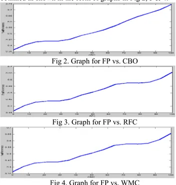
All the three input parameters WMC, RFC and CBO are directly proportional to fault proneness i.e. more the WMC, RFC and CBO more will be fault proneness. After creating the rule base to depict the true picture following results were obtained as shown in the form of graphs in Fig 2, 3 & 4.
Fig 2. Graph for FP vs. CBO
Fig 3. Graph for FP vs. RFC
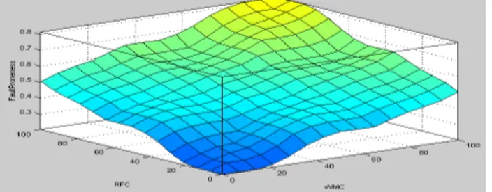
The surface view of fault proneness and other three input parameters WMC, RFC and CBO is obtained after the implication of the rules from the rule base. The monotonicity of the surface depends on the rule base. For better results the surface should be monotonous and symmetrical as obtained in the Fig 5 and 6.
Fig 5. Surface view of FP, RFC and WMC
Fig 6. Surface View of FP, WMC and CBO
VII. TESTING OF THE PROPOSED FAULT
PRONENESS PREDICTION SYSTEM
The testing of the algorithm is done by viewing rules on a rule viewer crisp value as input is given to the three input parameters and the output is obtained. Let us consider a class whose value for WMC is 17, value for RFC is 24 and Value for CBO is 7. To determine how much fault prone the class is these values are fed to the rule viewer and the role viewer will appear to be like as shown in Fig 7. The fault proneness of the class is 0.203 i.e. there is 0.2 probability that fault will be found in the class. This value has been obtained after firing the rule base and after Defuzzification.
Fig 7. Rule Viewer
VIII. PROPOSED ALGORITHM FOR DETERMINING THE DEFECT DENSITY (DD)
The predictive model used here to predict the defect density is given by Abreu et al. in [1]. That predictive model is further implemented with the help of Fuzzy Tool Box using Matlab Software. As per the above-mentioned model DD is given by:
DD = DD +MHF MHF + AHF AHF + MIF MIF + AIF AIF+POF POF +COF COF + DD
Where MOOD metrics = independent variables DD = outcome variables = response coefficient. = intercept parameter
DD = random error (taken to be zero) The value of these parameters according to Abreu et al. is shown in table 1
Table 1: Response Coefficients and Intercept Parameter
Metrics
MHF 10.958
AHF -0.649
MIF 2.194
AIF -7.564
POF -24.194
COF 29.959
2.643
The above mentioned formula has been used to predict the defect density of the software module using fuzzy logic. An algorithm consisting of various steps have been proposed as shown in the next section.
A. Input Parameters
The input parameters involve the computation of MOOD Metrics. As explained earlier the MOOD Metrics consists of six metrics. The metrics of the MOOD suite are Method Inheritance Factor, Attribute Inheritance Factor, Method Hiding Factor, Attribute Hiding Factor, Polymorphism Factor and Coupling Factor. These metrics are related to the defect density as shown in Eq given by Abreu et al. in [1]. The response of the factors to defect density has also been shown in table 1
B. Design of Fuzzification Module
Linguistic variables are then assigned to the input parameters based on their values. The assignment of the linguistic variables depends on the range of the input measurement.
Linguistic Variables for input variables
same and is shown as under. Consider an example of membership plot of MHF. Rests of the five membership plots are of the same type.
[Input1]
Name='MHF'
Range=[0 1] NumMFs=3
MF1='low':'trimf',[0 0 0.4] MF2='mid':'trimf',[0.1 0.5 0.9] MF3='high':'trimf',[0.6 1 1]
Linguistic Variables for Defect Density
The main difference which lies between the Mamdani and Sugeno model is the output membership function. The output membership function for Sugeno model is only linear and constant. Here in defect density we are using linear membership function for low, mid and high values. Low is linear membership function with the values which are assigned to it. The range which is assigned to the linguistic variables is shown under.
[Output1]
Name='Defect__Density'
Range=[0 1] NumMFs=3
MF1='low':'linear',[10.958 -0.649 2.194 -7.564 -24.194 29.959 2.643]
MF2='mid':'linear',[10.958 -0.649 2.194 -7.564 -24.194 29.959 2.643]
MF3='high':'linear',[10.958 -0.649 2.194 -7.564 -24.194 29.959 2.643]
C. Design of Knowledge Base
The knowledge base is designed in the same way as it is designed earlier to find fault proneness.
D. Defuzzification
The input to the defuzzification process is the rule base and the output is the crisp values given after performing the defuzzification using the “wtaver” method. Here after the defuzzification process the value obtained is the Defect Density, which means number of defects per KSLOC.
IX. EXPERIMENTAL RESULTS
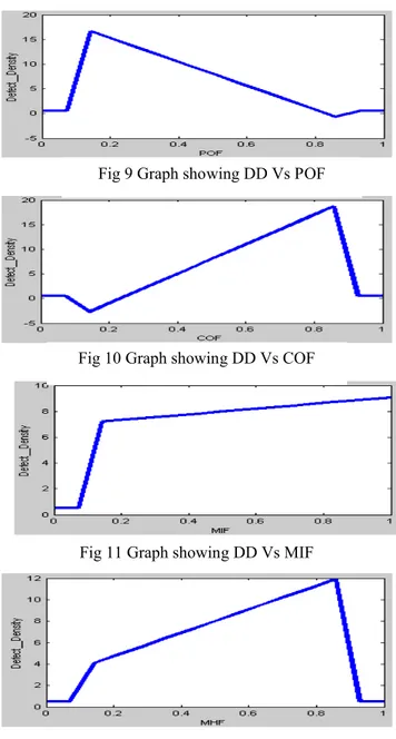
Among all the six input parameters some have shown to be directly proportional and some inversely proportional to defect density. After creating the rule base to depict the true picture following results were obtained shown in the form of graphs in Fig 8,9,10,11,12,13..
The surface view of Defect Density and other six input parameters MHF, AHF, MIF, AIF, POF, and COF is obtained after the implication of the rules from the rule base as shown in Fig 14, 15, 16, 17, 18.
Fig 10 Graph showing DD Vs COF
Fig 11 Graph showing DD Vs MIF
Fig 8 Graph showing DD Vs AIF
Fig 9 Graph showing DD Vs POF
Fig 12 Graph showing DD Vs MHF
The monotonicity of the surface depends on the rule base. Here the top of the surface has come out to be geometrically straight because the output linguistic variable is a linear function. For better results the surface should be
monotonous and symmetrical as obtained in the figures above.
X. TESTING OF THE PROPOSED DEFECT DENSITY PREDICTION SYSTEM
The testing of the algorithm is done by viewing rules on a rule viewer crisp value as input is given to the three input parameters and the output is obtained. Let us consider a class whose value for MHF is 36.4%, AHF is 95.7%, MIF is 38.2%, AIF is 22.4%. POF is 6% and COF is 2.3%. These values are fed to the rule viewer and the output is obtained in terms of defect density i.e. defects per KSLOC. As shown in the Fig 19 the defect density of the system is 4.38. The value which is shown here is the same as the values obtained by Abreu et al. in [1]. This value has been obtained after firing the rule base and after defuzzification.
So in this way fuzzy logic can be used to find the Defect Density of the system using MOOD Metrics. The prediction of the defect density can hence be used to concentrate on the module which has got more defects as per the Pareto principle
Fig 19 Rule Viewer for Defect Density
ACKNOWLEDGMENT
S. K. Khalsa thanks the Dept. of Comp. Sc. & Engg. of Guru Nanak Dev Engineering College, Ludhiana (Punjab, India) for providing the necessary resources for carrying out the research work
REFERENCES
[1] Fernando Brito e Abreu and Walcelio Melo.” Evaluating the impact of Object Oriented Design on Software Quality.” Proceedings of IEEE (METRICS’96)
[2] Lionel C. Briand, Jurgen Wust, Hakim Lounis, “Investigating Quality Factors in Object Oriented Design: An industrial case Study”. Proc Int’l Conf. Software Eng. pp 345-354, 1999.
[3] Lionel C. Briand, Jurgen Wust, Hakim Lounis, “Using Coupling Measurement for Impact Analysis in Object-Oriented Systems.” [4] Victor R. Basili, Lionel Briand, “A Validation of Object Oriented
Design Metrics as Quality Indicators” IEEE Trans. Software Engg.,vol.22,pp.751-761, 1996.
Fig 14 Surface View of DD, MIF and AHF
Fig 17 Surface View of DD, MIF & COF
Fig 18 Surface View of DD, AHF & COF Fig 15. Surface View of DD, MHF & MIF