Abstract—Robust loop shaping control is a feasible method for designing a robust controller; however, the controller designed by this method is complicated and difficult to implement practically. To overcome this problem, in this paper, a new design technique of a fixed-structure robust loop shaping controller for a highly maneuverable airplane, HIMAT, is proposed. The performance and robust stability conditions of the designed system satisfying H∞ loop shaping control are formulated as the objective function in the optimization problem. Particle Swarm Optimization (PSO) technique is adopted to solve this problem and to achieve the control parameters of the proposed controller. Simulation results demonstrate that the proposed approach is numerically efficient and leads to performance comparable to that of the other method.
Index Terms— H∞ loop shaping control, robust control, particle swarm optimization, HIMAT system, fixed-structure controller.
I. INTRODUCTION
In the past decades, many immense developments in robust control techniques have been proposed and the results of those are utilized in many control systems. As shown in previous works, H∞ optimal control is a powerful technique to design a robust controller for system under conditions of uncertainty, parameter change, and disturbance. However, the order of controller designed by this technique is much higher than that of the plant. It is not easy to implement this controller in practical applications. In industrial applications, structures such as PID, lead-lag compensators are widely used because their structures are simple, tuning parameters are fewer, and they are lower order. Unfortunately, tuning of control parameters of such controllers for achieving a good performance and robustness is difficult. To solve this problem, the design of fixed-structure robust controller has been proposed. Fixed-structure robust controller has become an interesting area of research because of its simple structure and acceptable controller order. However, the design of this controller by using analytical methods remains difficult. To simplify the problem, searching algorithms such as genetic algorithm, particle swarm optimization technique, tabu-search, etc., can be employed. Several approaches to
Manuscript received January 17, 2008. This work was supported in part by Faculty of Engineering, King Mongkut's Institute of Technology
Ladkrabang, Bangkok, Thailand.
Somyot is with the Department of Electrical Engineering, Faculty of Engineering, King Mongkut's Institute of Technology Ladkrabang, Bangkok 10520, Thailand. Email : [email protected]
Manukid is with the School of Engineering and Technology, Asian Institute of Technology, P.O. Box 4, Klong Luang, Pathumthani 12120, Thailand.
design a fixed-structure robust controller were proposed in [1-3, 5-7]. In [1], a robust H∞ optimal control problem with structure specified controller was solved by using genetic algorithm (GA). As concluded in [1], genetic algorithm is a simple and efficient tool to design a fixed-structure H∞ optimal controller. Bor-Sen.Chen. et. al.[2], proposed a PID design algorithm for mixed H2/H∞ control. In their paper, PID control parameters were tuned in the stability domain to achieve mixed H2/H∞ optimal control. A similar work was proposed in [3] by using the intelligent genetic algorithm to solve the mixed H2/H∞ optimal control problem. The techniques in [1-3] are based on the concept of H∞ optimal control which two appropriate weights for both the uncertainty of the model and the performance are essentially chosen. A difficulty with the H∞ optimal control approach is that the appropriate selection of close-loop objectives and weights is not straightforward [4]. Moreover, especially in MIMO system, it is not easy to specify the uncertainty weight in practice. Alternatively, MIMO controller can be designed by using H∞ loop shaping control [4] which is a simple and efficient technique for designing a robust controller. Uncertainties in this approach are modeled as normalized co-prime factors; this uncertainty model does not represent actual physical uncertainty, which usually is unknown in real problems. This technique requires only two specified weights, pre- and post-compensator weights, for shaping the nominal plant so that the desired open loop shape is achieved. Fortunately, the selection of such weights is based on the concept of classical loop shaping which is a well known technique in the controller design. By the reasons mentioned above, this technique is simpler and more intuitive than other robust control techniques. However, the controller designed by H∞ loop shaping is still complicated. To overcome this problem, several approaches have been proposed to design a fixed-structure H∞ loop shaping controller, such as a state-space approach by A. Umut. Genc in 2000 [5], genetic algorithms based fixed-structure H∞ loop shaping by Somyot and Manukid in 2004 [6], etc. The method in [5] is based on the concept of state space approach and BMI optimization. Unfortunately, the chance of reaching a satisfactory solution of this approach depends on the initial controller chosen and the problem of the local minima is often occurred. In [6], a global optimization method was adopted to design the fixed-structure robust H∞ loop shaping controller; however, the designed controllers in [6] were only implemented on a pneumatic servo system which is a SISO system. In [7], the same technique as [6] was adopted to design a robust controller of a boost converter; however, this application is also a SISO system. In this paper, PSO is proposed to synthesize a fixed-structure H∞ loop shaping controller for HIMAT system. Based on the concept of PSO technique, the choosing of initial controller required in the method in [5] is not necessary and the problem of local minima is reduced.
Structured Robust Loop Shaping Control For HIMAT
System Using Swarm Intelligent Approach
Structure of controller in the proposed technique is selectable; in this paper, two fixed-structure controllers, centralized and decentralized PID controllers, are designed. Simulation results show that the controller designed by the proposed approach has a good performance and robustness as well as simple structure. This allows our designed controller to be implemented practically and reduces the gap between the theoretical and practical approach.
The remainder of this paper is organized as follows. Conventional H∞ loop shaping and the proposed technique are discussed in section 2. PSO algorithm is also described in this section. Section 3 demonstrates a design example and results. And, finally, in section 4 the paper is summarized with some final remarks.
II. H∞LOOP SHAPING CONTROL AND PROPOSED TECHNIQUE
This section illustrates the concepts of conventional H∞ loop shaping control and the proposed technique.
A. Conventional H∞ Loop Shaping Control
H∞ loop shaping control is an efficient method to design a robust controller. This approach requires two weighting functions, W1(pre-compensator) and W2(post-compensator), for shaping the original plant G0 so that the desired open loop shape is achieved. In this approach, the shaped plant is formulated as normalized co-prime factor, which separates the shaped plant Gs into normalized nominator Ns and denominator Ms factors [8].
1 2
K
=
W K W
∞2 1
S
G
=
W GW
1
W
G
K
∞2
W
Fig. 1. H∞ loop shaping design.
The following steps can be applied to design H∞ loop shaping controller [4].
Step 1 Shape the singular values of the nominal plant Goby using a pre-compensator W1 and/or a post-compensator W2 to get the desired loop shape. W2 can be chosen as a constant since the effect of the sensor noise is negligible when the use of good sensor is assumed [9].
Gs = W2G0W1=
N M
s s1 −. (1) Based on the concept of H∞ loop shaping, the perturbed plant is written as
1
( s Ns)( s M s)
GΔ= N + Δ M + Δ − (2) where ΔNs and ΔMs are stable, unknown representing the uncertainty satisfying Δ ΔNs, Ms ∞≤
ε
,ε
is the uncertainty boundary called stability margin. There are some guidelines for selecting the weight available in [9].Step 2 Calculate εopt, where
(
)
1 1( inf [ ] )
opt s s
K stabilizing
I
I G K I G
K
ε
− −∞
∞ ∞
⎡ ⎤
= ⎢ ⎥ −
⎣ ⎦ (3)
To determine εopt, there is a unique method explained in appendix A. εopt << 1indicates that W1or W2 designed in step 1 are incompatible with robust stability requirement. To ensure the robust stability of the nominal plant, the weighting functions are selected so that εopt ≥ 0.25 [9]. If εopt is not satisfied, then go to step 1, adjust the weighting functions. Step 3 Select ε < εopt and then synthesize a controller K∞ that satisfies [4]
∞ zw
T
=(
)
1 1[
]
s s
I
I
G K
I
G
K
ε
− −
∞
∞ ∞
⎡
⎤
−
≤
⎢
⎥
⎣
⎦
(4)where
T
zw ∞is the infinity norm from the disturbances w to state z. Controller K∞ is obtained by solving the sub-optimal control problem in (4). The details of this solving are available in [8].Step 4 Final controller (K) is determined as follow
K = W1K∞W2 (5) Fig. 1 shows the controller in H∞ loop shaping control.
B. PSO based Fixed-Structure H∞ Loop Shaping Optimization
In the proposed technique, PSO is adopted to design a fixed-structure robust controller. A similar work was presented in [5]. However, the problem in [5] was formulated by using a BMI-based optimization approach unlike the PSO approach taken in this paper. In [5], initial solution required in the design procedure strongly influences the performance of final solution. Moreover, there is no systematic method to select such initial value. In the proposed technique, the design is more flexible than the previous work [5] by selecting the appropriate upper and lower bounds of solution. In the design, boundary of solution of PSO is selected by considering the pre-compensator weight. Normally, this weight is specified by first or second order transfer functions at the diagonals entries of W1. Fortunately, it is not difficult to transform these transfer functions to PI/PID structure. Since the fixed-structure controller in the paper is PID, thus, the choosing of boundary of solution by considering weight, W1, can be done easily. In addition, because PSO technique is based on the concept of global optimization searching, the problem of local minima is reduced.
1 1 2 2
( 1) ( ) [ ( ( )] [ ( ( )]
i i i pi i i i
v iter+ =Qv iter +α γ X −X iter +α γ G−X iter
(6) where Q is the momentum coefficient,
v
iis the velocity of ith particle, iter is the iteration count,α
1 andα
2 are the specified acceleration coefficients, Xpi is the best position found by ith particle, G is the best position found by swarm (global best),γ
1i andγ
2i are the random numbers in the range [0,1]. Note that the velocity must be within the specified range [Vmin , Vmax]. If not, set it to the limiting values. As shown in (6), there are three terms in the equation. By these terms, the advantages of local minimum searching, global minimum searching, local optima avoidance and the information sharing among particles are achieved and the particle can reach the best solution. The details of PSO are available in [10].Fig. 2 The movement of a swarm.
In the proposed technique, although the controller is structured, it still retains the entire robustness and performance guarantee as long as a satisfactory uncertainty boundary εis achieved. The proposed algorithm is explained as follows. Assume that the predefined structure controller K(p) has satisfied parameters p. Based on the concept of H∞ loop shaping, optimization goal is to find parameters p in controller K(p) that minimize infinity norm from disturbances w to states z,
T
zw ∞ . In the proposed technique, the final controller K is defined asK = K(p)W2 (7) Assuming that W1 are invertible, from (5) then it is obtained that
K∞ =
W
1−1K(p) (8) In many cases, the weight W2is selected as identity matrix I. However, if W2is a transfer function matrix, then the final controller is the controller K(p) in series with the weight W2. By substituting (8) into (4), the ∞-norm of the transfer function matrix from disturbances to states,T
zw ∞, which is subjected to be minimized can be written as(
)
1cos 1 2 0
1
( ) [ ]
( )
t zw s
I
J T I W G K p I G
W K p
γ
−− ∞
∞
⎡ ⎤
= = = ⎢ ⎥ −
⎣ ⎦
The optimization problem can be written as
Maximize
(
)
1 1
2 0 1
1
( ) [ ]
( ) s
I
I W G K p I G
W K p
− −
−
∞
⎡ ⎤
−
⎢ ⎥
⎣ ⎦
Subject to pi,min <pi<pi,max,
where
p
i,min andp
i,max are the lower and upper bound values of the parameter pi in the parameter vector p, respectively. Thus, the fitness function in the controller synthesis can be written as(
)
1 1
2 0 1
1
( ) [ ]
( ) Fitness (J)
if stabilizes the plant 0.0001 otherwise
s
I
I W G K p I G W K p
K
− −
−
∞∞
⎧⎛ ⎡ ⎤ ⎞
⎪⎜⎜ ⎢ ⎥ − ⎟⎟ ⎪ ⎣⎝ ⎦ ⎠ = ⎨
⎪ ⎪ ⎩
(9) The fitness is set to a small value (in this case is 0.0001) if K does not stabilize the plant. Our proposed algorithm is summarized as follows.
-Weight Selection
Step 1 Select the weights W1 and W2 to achieve the performance and desired loop shape.
Step 2 Evaluate εopt using (3). If εopt < 0.25, then back to step 1 to change the weights.
-Controller synthesis
Step 3 Select a controller structure K(p) and define the PSO parameters and control parameter ranges. Initialize several sets of parameters p as swarm in the 1st iteration. In this case, each p is a particle.
Step 4 Use the PSO to find the optimal control parameter, p*. Step 5 Check performances in both frequency and time domains. If the performance is not satisfied such as too low ε (too low fitness function), then go to step 3 to change the structure of controller. Low ε indicates that the selected control structure is not suitable for the problem.
Standard PSO algorithm used in step 4 of the proposed technique is briefly described as follows.
Specify the parameters in PSO such as population size (n), upper and lower bound values of problem space, fitness function (J), maximum and minimum velocity of particles (Vmaxand Vmin, respectively), maximum and minimum inertia weights (
Q
maxandQ
min, respectively).1. Initialize n particles with random positions within upper and lower bound values of the problem space. Set iteration count as iter =1.
2. Evaluate the fitness function (J) of each particle using (9).
3. For each particle, find the best position found by particle i call it Xpi and let the fitness value associated with it be Jpbesti. At first iteration, position of each particle and its fitness value of ith particle are set to Xpi and Jpbesti, respectively.
4. Find a best position found by swarm call it G which is the position that maximum fitness value is obtained. Let the fitness value associated with it be JGbest. To find G the following algorithm described by pseudo code is adopted.
(At first iteration set Jgbest,=0) For i = 1 to n do
If Jpbesti > Jgbest, then
end;
5. Update the inertia weight by following equation max min
max
max
Q
Q
Q
Q
iter
iter
−
=
−
where Q is inertia weight,
iter
anditer
maxare the iteration count and maximum iteration, respectively. 6. Update the velocity and position of each particle. For the particle i, theupdated velocity and position can be determined by following equations.1 1 2 2
( 1) ( ) [ ( ( )] [ ( ( )]
( 1) ( ) ( 1)
i i i pi i i i i i i
v iter Qv iter X X iter G X iter
X iter X iter v iter
α γ α γ
+ = + − + − + = + +
7. Increment iteration for a step. (iter = iter+1) 8. Stop if the convergence or stopping criteria are met,
otherwise go to step 2.
III. SIMULATION RESULTS
In this paper, the design of pitch axis controller for an experimental highly maneuverable airplane, HIMAT, is studied. The dynamic model of this plant is taken from the
μ-synthesis and analysis toolbox user’s guide [11]. The state vector of this plant consists of the four variables which are forward velocity, angle-of-attack, pitch rate, and pitch angle. The control inputs are the elevon and the canard. The measured variables are angle-of-attack and pitch angle. The details of this plant are given in appendix B. The design objective is to reject disturbances up to about 1 rad/s in the presence of substantial plant uncertainty above 100 rad/s [5]. In this problem, the pre- and post-compensator weights are chosen as [5].
1 2
1
0
1 0
0.001 ,
1 0 1
0
0.001
s s
W W
s s +
⎡ ⎤
⎢ + ⎥ ⎡ ⎤
=⎢ ⎥ =⎢ ⎥
+ ⎣ ⎦
⎢ ⎥
⎢ + ⎥
⎣ ⎦
(10)
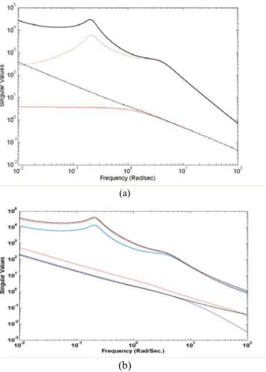
Singular values of HIMAT and desired loop shape are plotted in Fig. 3 (a). As seen in this figure, the bandwidth and performance are significantly improved by the compensator weights. The shaped plant has large gains at low frequencies for performance and small gains at high frequencies for noise attenuation. With these weighting functions, the robust requirement is satisfied.
By using (3), the optimal stability margin of the shaped plant is found to be 0.436. This value indicates that the selected weights are compatible with robust stability requirement in the problem. To design the HLS controller, stability margin 0.3964 is selected. As a result, the final controller (full order HLS controller) is 7th order and complicated.
(a)
(b)
Fig. 3. Open loop shape of (a) the nominal plant (Red line) and shaped plant (Black line) (b) the loop shape by the proposed controllers (Red line: Centralized PID, dash line: Decentralized PID) and HLS (Blue line).
Next, two fixed-structure robust controllers are designed. The structure of controllers is selected as PID with first-order derivative filter. Accordingly, these controllers are simple and easy to implement in real applications. These controllers are expressed in (11) and (12) for centralized and decentralized controllers, respectively. Kp, Ki, Kd, and τd are parameters to be evaluated.
Centralized controller:
( )
1 1 2 2
1 2
3 3 4 4
3 4
1 2 1 2 1 2
3 4 3 4 3 4
1 1
1 1
, ,
i d i d
p p
d d
i d i d
p p
d d
p p i i d d
p i d
p p i i d d
K K s K K s
K K
s s s s
K p
K K s K K s
K K
s s s s
K K K K K K
K K K
K K K K K K
τ τ
τ τ
⎡ + + + + ⎤
⎢ + + ⎥
⎢ ⎥
=
⎢ + + + + ⎥
⎢ + + ⎥
⎣ ⎦
⎡ ⎤ ⎡ ⎤ ⎡ ⎤
=⎢ ⎥ =⎢ ⎥ =⎢ ⎥
⎣ ⎦ ⎣ ⎦
⎣ ⎦
Decentralized controller:
( )
1 1
1
4 4
4
1 1 1
4 4 4
0 1
0
1
0 0 0
, ,
0 0 0
i d p
d
i d p
d
p i d
p i d
p i d
K K s
K
s s
K p
K K s
K
s s
K K K
K K K
K K K
τ
τ
⎡ + + ⎤
⎢ + ⎥
⎢ ⎥
=
⎢ + + ⎥
⎢ + ⎥
⎣ ⎦
⎡ ⎤ ⎡ ⎤ ⎡ ⎤
=⎢ ⎥ =⎢ ⎥ =⎢ ⎥
⎣ ⎦ ⎣ ⎦
⎣ ⎦
(12)
In the optimization problem, the upper and lower bounds of control parameters and PSO parameters are set as follows: Kp∈ [-10, 10], Ki∈ [-10, 10], Kd∈ [-5, 5], τd∈ [0.01, 1], population size = 300, minimum and maximum velocities are 0 and 2 respectively, acceleration coefficients = 2.1, minimum and maximum inertia weights are 0.6 and 0.9, respectively, maximum iteration = 80. As shown in the above mentioned control parameter ranges, the selection of upper and lower bounds is easily carried out by observing the performance weight
W
1. After running the PSO for 80 iterations, the optimal control parameters are found to beCase I: Centralized controller.
d
0.52601 0.14172 1.96082 0.28352
, ,
0.47833 0.70387 2.2261 1.224
0.007434 0.006844
, 0.0068479
0.006272 0.0016058
p i
d
K K
K τ
−
⎡ ⎤ ⎡ ⎤
=⎢ ⎥ =⎢ ⎥
− −
⎣ ⎦ ⎣ ⎦
⎡ ⎤
=⎢ ⎥ = −
⎣ ⎦
(13)
Case II: Decentralized controller.
d
0.5367 0 1.488 0
, ,
0 0.5659 0 0.4909
0.01569 0
, 0.0085855
0 0.00499
p i
d
K K
K τ
⎡ ⎤ ⎡ ⎤
=⎢ ⎥ =⎢ ⎥
− −
⎣ ⎦ ⎣ ⎦
⎡ ⎤
=⎢ ⎥ = −
⎣ ⎦
(14)
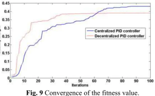
Note that all of the designed controllers in this paper are the controllers in positive feedback control system. Fig. 8 (b) shows comparison of the loop shapes by the proposed controllers and HLS. As seen in this figure, all loop shapes are close to the desired loop shape. Fig. 9 shows plots of convergence of objective function (stability margin) versus iterations by PSO. As seen in this figure, the stability margins obtained from the proposed centralized and decentralized controllers are 0.432 and 0.389, respectively. These values indicate that the robust stability and performance of the designed systems are satisfied.
Fig. 9 Convergence of the fitness value.
In this simulation studies, the robustness and performance of the proposed controllers are compared with those of the controller obtained from [5], that is.
d
1.3074 0.0601 1.2729 0.0795
, ,
1.3414 1.3123 1.3609 1.2921
0.0077 0.0043 1
,
0.0069 0.0039 99.5724
p i
d
K K
K τ
− −
⎡ ⎤ ⎡ ⎤
=⎢ ⎥ =⎢ ⎥
− −
⎣ ⎦ ⎣ ⎦
⎡ ⎤
=⎢ ⎥ = − −
⎣ ⎦
(15)
Table 1 Comparisons of the stability margins obtained from the controllers in Example 2.
Controller Stability Margin
1. Proposed Controller:
1.1 Centralized PID Controller 0.432
1.2 Decentralized PID Controller 0.389
2. Robust Centralized PID Controller designed by BMI optimization [5] 0.309 The stability margin obtained by the above controller is
0.309. Clearly, the stability margin of the proposed centralized controller is also much better than that of the controller in [5].
Table 1 summarizes the results of stability margin obtained from the proposed controller and others. As the results, the stability margin from the proposed centralized PID controller is better than that of other controllers. Accordingly, the proposed technique is an efficient method to design a fixed-structure robust loop shaping controller. Note that the design of decentralized PID controller was not presented in the previous work [5].
IV. CONCLUSIONS
In this paper, a PSO based fixed-structure H∞ loop shaping controller for HIMAT system is proposed. Based on the concept of conventional H∞ loop shaping, only a single
optimal solution. Simulation results demonstrate that the proposed technique is valid and flexible.
APPENDIX A
Given a shaped plant Gs and A, B, C, D represent the shaped plant in the state-space form. To determine εopt, there is a unique method as follows [8].
2 / 1 max 1
)) ( 1
( XZ
opt
opt
ε
λ
γ
= − = +where X and Z are the solutions of two Riccati in (A.1) and (A.2) respectively, λmax is the maximum eigenvalue.
1 1 1 1
( T ) ( T )T T T 0
A BS D C Z− − +Z A BS D C− − −ZC R CZ− +BS B− =
(A.1)
1 1 1 1
( T )T ( T ) T T 0
A BS D C− − X+X A BS D C− − −XBS B X− +C R C− =
(A.2) where S=I+DTD, R = I+DDT
APPENDIX B
The state vector of HIMAT model consists of vehicle’s rigid body variables.
[
, , , ]
T
x
=
δ α θ
v
q
where
δ
v
is the forward velocity,α
is angle between velocity vector and aircraft's longitudinal axis, q is rate-of-change of aircraft attitude angle, and θ is the aircraft attitude angle. The state space of HIMAT can be written asx
Ax
Bu
y
Cx
Du
•
=
+
=
+
The control inputs are the elevon and the canard. The measured variables are angle-of-attack and pitch angle. In this paper, the linearlized model is taken from [11], that is
0.0226 36.6 18.9 32.1
0 1.9 0.983 0
,
0.0123 11.7 2.63 0
0 0 1 0
0 0
0.414 0
, 77.8 22.4
0 0
0 57.3 0 0
,
0 0 0 57.3
0 0
0 0
A
B
C
D
− − − −
⎡ ⎤
⎢ − ⎥
⎢ ⎥
=
⎢ − − ⎥
⎢ ⎥
⎣ ⎦
⎡ ⎤ ⎢− ⎥ ⎢ ⎥ =
⎢− ⎥ ⎢ ⎥ ⎣ ⎦
⎡ ⎤
= ⎢⎣ ⎥⎦
⎡ ⎤ = ⎢ ⎥ ⎣ ⎦
ACKNOWLEDGMENT
This research work is financially supported by the Thailand Research Fund (Project No. MRG4980087).
REFERENCES
[1] B. S. Chenand Y. M. Cheng., A structure-specified optimal control design for practical applications: a genetic approach, IEEE Trans. on Control System Technology, 6(6),1998, 707-718.
[2] B. S. Chen,, Y.-M. Cheng, and C. H. Lee., A genetic approach to mixed H2/ H∞ optimal PID control, IEEE Trans. on Control Systems, 1995, 51-60.
[3] S. J. Ho, S. Y. Ho, M. H. Hung, L. S. Shu, and H. L. Huang, Designing structure-specified mixed H2/ H∞ optimal controllers using an intelligent genetic algorithm IGA, IEEE Trans. on Control Systems, 13(6), 2005, 1119-24.
[4] D.C. McFarlane and K. Glover., A loop shaping design procedure using H∞ synthesis, IEEE Trans. On Automatic Control, 37(6), 1992, 759–769.
[5] A. U. Genc, A state-space algorithm for designing H∞ loop shaping PID controllers, tech. rep., Cambridge University, Cambridge, UK, Oct. 2000.
[6] S. Kaitwanidvilai and M. Parnichkun, Genetic algorithm based fixed-structure robust H∞ loop shaping control of a pneumatic servo system, International Journal of Robotics and Mechatronics, 2004, 16(4).
[7] S. Kaitwanidvilai and P. Olranthichachat, Genetic based Robust H∞
Loop Shaping PID Control for a Current-Mode Boost Converter,
ICEMS2006, November 2006, Japan.
[8] K. Zhou, J. C. Doyle., Essential of Robust Control (New Jersey: Prentice-Hall, 1998).
[9] S. Skogestad, I. Postlethwaite, Multivariable Feedback Control Analysis and Design. (2nd
ed. New York: John Wiley & Son, 1996). [10] J. Kennedy and R. Eberhart, Particle swarm optimization, IEEE
International Conference on Neural Networks, 4, 1995, 1942-1948. [11] G.J. Balas, J.C. Doyle, K. Glover, A. Packard, and R. Smith.