A Mixed-Effects Model with Different
Strategies for Modeling Volume in
Cunninghamia lanceolata
Plantations
Mei Guangyi1, Sun Yujun1*, Xu Hao1, Sergio de-Miguel2,3
1Laboratory for Silviculture and Conservation, Beijing Forestry University, 35 Qinghua East Road, Beijing, China,2Faculty of Science and Forestry, University of Eastern Finland, P.O., Joensuu, Finland,
3Departament de Producció Vegetal i Ciència Forestal, Universitat de Lleida-Agrotecnio Center (UdL-Agrotecnio), Av. Rovira Roure, 191, E–25198, Lleida, Spain
Abstract
A systematic evaluation of nonlinear mixed-effect taper models for volume prediction was performed. Of 21 taper equations with fewer than 5 parameters each, the best 4-parameter fixed-effect model according to fitting statistics was then modified by comparing its values for the parameters total height (H), diameter at breast height (DBH), and aboveground height (h) to modeling data. Seven alternative prediction strategies were compared using the best new equation in the absence of calibration data, which is often unavailable in for-estry practice. The results of this study suggest that because calibration may sometimes be a realistic option, though it is rarely used in practical applications, one of the best strategies for improving the accuracy of volume prediction is the strategy with 7 calculated total heights of 3, 6 and 9 trees in the largest, smallest and medium-size categories, respectively. We cannot use the average trees or dominant trees for calculating the random parameter for fur-ther predictions. The method described here will allow the user to make the best choices of taper type and the best random-effect calculated strategy for each practical application and situation at tree level.
Introduction
The ability to describe the stem form of a forest tree is important for practical and theoretical reasons. Foresters require stem profile models for estimating the volume and the value of the whole stem or a part of it [1], to various utilization limits [2,3]. Such estimates are essential in forest planning, for example in evaluating the economics of different management regimes [4]. A theoretical aspect of interest is the relationship between stem form, competition and tree age for individual species, which calls for parameter-parsimonious models that can be used to make general statements about the effect of silviculture and site conditions on stem form [5,6].
Taper models can be classified into simple polynomial, segmented and variable-form mod-els [7]. A comparison of these 3 types of modmod-els shows that although the simple polynomial
OPEN ACCESS
Citation:Guangyi M, Yujun S, Hao X, de-Miguel S (2015) A Mixed-Effects Model with Different Strategies for Modeling Volume inCunninghamia lanceolataPlantations. PLoS ONE 10(10): e0140095. doi:10.1371/journal.pone.0140095
Editor:RunGuo Zang, Chinese Academy of Forestry, CHINA
Received:June 26, 2015
Accepted:September 22, 2015
Published:October 7, 2015
Copyright:© 2015 Guangyi et al. This is an open access article distributed under the terms of the Creative Commons Attribution License, which permits unrestricted use, distribution, and reproduction in any medium, provided the original author and source are credited.
Data Availability Statement:All relevant data are within the paper and its Supporting Information files.
Funding:This study was supported by the project of forestry science and technology research (No. 2012-07) and the National Technology Extension Fund of Forestry ([2014]26).
taper models have a notably simple structure and easy convergence, they are not good at accu-rately describing the stem. The segmented taper models are more complicated and have good accuracy but are also more difficult to calculate. The variable-form taper models have good structure, can accurately predict the stand volume, and are not overly complicated to calculate [8–10]. Therefore, in contrast to the single taper and segmented taper models, the variable-form taper model is widely used.
Because the data for stem taper have hierarchy and repeated measurement [11], many researchers use Nonlinear Mixed-Effects (NLME) models to develop taper models. Compared with the regression method, NLME models consist of fixed- and random-effect parameters and have the advantage of enabling the modeling of the covariance matrix of correlated data. There are 2 responsible variable components in the variance-covariance matrix: the random-effect component and the within-subject component. Both components can be used to model the heteroskedasticity and autocorrelation of a mixed-effect model [12–14].
However, previous studies have mostly considered the fitting of one variable exponent [15]. Many studies [15–21] used the segmented model of Max and Burkhart (1976) [22]. Further-more, de-Miguel[4] compared the simple polynomial, segmented and variable-form taper model types using both fixed- and random-effect approaches to predict the volume. Finally, Kozak II with 9 parameters [13] was selected as the best taper model. However, the taper model of Kozak II has 9 parameters and a complicated structure. Therefore, there is no systematic comparison of the aforementioned taper models using fixed- and random-effect approaches that has both simple structure and good accuracy.
For the mixed-effect model, the high cost of measuring additional upper-stem diameters makes it difficult to calibrate the tree-specific taper functions in forestry practice. To solve this problem, de-Miguel [23] compared 3 different prediction methods in model evaluation and validation: (1) a fixed-effect model, (2) the fixed part of a mixed-effect model, and (3) Monte Carlo simulation based on a randomized mixed-effect model. Their results suggest that fixed-effect models should be used when the purpose of the model is prediction and calibration data are not available. Crecente-Campogeneralized the NLME height—diameter model for Eucalyp-tus globulusL. in northwestern Spain [24]; random parameters for particular plots were esti-mated with different tree selections (5 options). Finally, the height—diameter relationships for individual plots were obtained by calibrating the height measurements of the 3 smallest trees in a plot.
First, this study aimed to perform a consistent analysis of the performance of taper models with fewer than 5 parameters and to modify each of them for good accuracy. Using the best model that was found, 7 strategies were compared for volume prediction using a taper model in the absence of additional measurements for tree-specific calibration [25].
Materials and Methods
Materials
species. So we confirm that the field studies did not involve endangered or protected species. The region is characterized by ferromagnesian (red) soils and has a mean annual precipitation of approximately 1699 mm, a mean annual frost-free season of 287 days, and a mean annual temperature of 18.7°C [26].
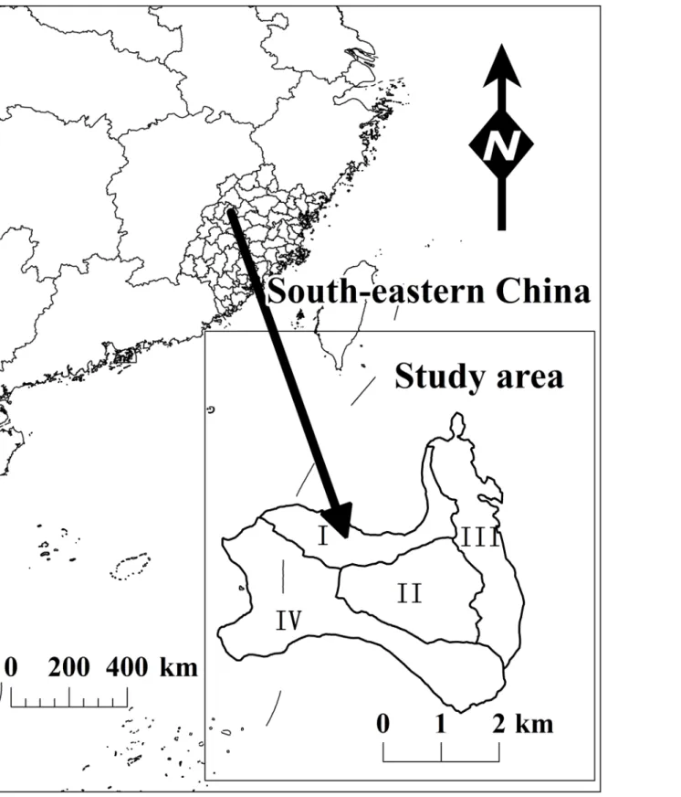
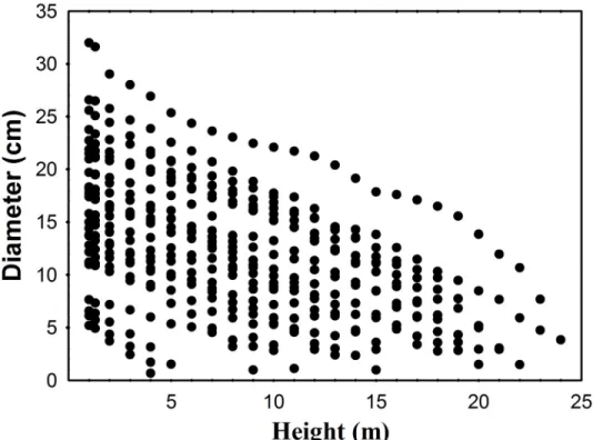
We sampled four regions, which were divided equally into 41 plots ofCunninghamia lan-ceolatatrees (Qiantan, 15 plots; Shuinan, 8 plots; Yuhua, 11 plots; and Yuandang, 9 plots) and are represented by I, II, III and IV, respectively, inFig 1. Established between 2010 and 2014, the plots vary in size from 400 to 600 m2. In the plots, we measured the diameters at breast height (DBHs) over the bark (at 1.3 m above ground) of fresh trees (height>1.3 m) and the total tree height of 41 trees that were felled for stem analysis. Before felling each tree, we mea-sured two attributes: diameter at breast height (1.3 m above ground) and total tree height (H). After felling, we measured the diameter at intervals of 1 m and 2 m above the breast height depending on the total tree height. We further performed a laboratory analysis of the outer and inner bark of each disc. These diameters were measured along the largest axis and smallest axis (Table 1andFig 2).
Selection of candidate equations
The ranking and selection of the taper models were performed in three steps. First, 21 pub-lished candidate equations are variable-form taper models with fewer than 5 parameters (Tables2and3) [27]. The best function was selected by applying 5 statistical criteria: Mean Absolute Bias (MAB), root mean square error (RMSE), adjusted coefficient of determination R2, Akaike’s information criterion (AIC), and Bayesian information criterion (BIC) [28].
Second, we modified the best model because building an equation with fewer parameters while maintaining good accuracy in volume prediction was the main goal of this study. The model was modified by comparing the relationships among the total height (H), diameter at breast height (DBH), and height above ground level (h) against the modeling data. The best taper model for d2provides unbiased predictions for the cross-sectional area and volume [29– 30]. Therefore, all fitted candidate models used dkias the ith diameter measurement [4]:
d2
ki¼fðhki;Dk;Hk;qÞ þεki ð1Þ
where dkiis the ith diameter measurement of tree k, which is measured at height hki, Dkand Hk
are the DBH and total height of tree k, respectively, q is the vector of 1–5 parameters, andεkiis the residual.
Volume calculation based on taper model
Based on taper model selected above,Formula (2)was used calculate the volume of trees.
p
40000 ðH
0 d2
dh ð2Þ
where H is the total height, d is the diameter outside the bark at height h (cm), h is the height above ground level.
Testing different prediction strategies using different random parameters
Fig 1. 4 sites of Fujian province, Southeast China, where 41 trees were sampled.
from 1 to 10 for random parameter calculation in model calibration and using the remaining trees for validation in 7 strategies. The 7 selected alternatives are as follows:
1. calculating a fixed-parameter model (with no random-effect parameter).
2. calculating the fixed part of a mixed-effect model (random-effect parameter is 0).
3. calculating the heights of the randomly selected trees (total heights of 1–10 randomly selected trees to calculate the parameters).
4. calculating the heights of the largest selected trees (calculating the total heights of 1–10 larg-est trees to calculate the parameter).
5. calculating the heights of the smallest selected trees (total heights of 1–10 smallest trees to calculate the parameters).
Table 1. Summary of tree attributes for theCunninghamia lanceolate.
DBH(cm) Total height(m) Disk dob (cm) Disk height(m)
Mean 17.3 17.3 12.0 7.7
SD 5.8 5.5 6.0 5.9
Minimum 4.9 4.1 0.7 0.0
Maximum 28.4 25.5 30.4 25.0
doi:10.1371/journal.pone.0140095.t001
Fig 2. Diameter and total height distribution of the 466 h-d data used from 41 trees to model the taper equations.
6. calculating the heights of the medium-size selected trees (total heights of 1–10 medium-size trees to calculate the parameters).
7. calculating the heights of a mix of selected trees (calculating the total heights of 3, 6 and 9 trees in the largest, smallest and medium-size categories) [4,22,24].
Table 2. List of 21 candidate taper models, which were classified according to the number of parame-ters (NP) developed in this study.
NP Models evaluated
1 Kozak et al. (a) (1969)[31],Ormerod(1973)[32], Demearchalk (a) (1972)[33]
2 Kozak et al. (b) (1969)[31],Biging(1984)[34], Newberry and Burkhart (a) (1986)[35], Newberry and Burkhart (b) (1986), Reed and Green[36], Forslund (1990)[37]
3 Coffre(1982)[38], Kozak1969(c)[31], Real and Moore (1986)[39], Manuel(2015) [40]
4 Bennett and Swindel(1972)[41], Demaerschalk (b) (1972)[33], Demaerschalk (b)(1973)[42],Zeng Weisheng(1997)[43], Sharma(2009)[44], Goulding and Murray (1976)[45]
5 Lee et al. (2003)[46], Cervera (1973)[47] doi:10.1371/journal.pone.0140095.t002
Table 3. The 21 candidate equations and their corresponding mathematical expressions.
Eq. Model Expression
1 Zeng Weisheng (1997) d=D¼Xðb1þb2z0:25þb3z0:5þb4ðD=HÞÞ
2 Sharma (2009) d=D¼b1ððH hÞ=ðH 1:37ÞÞðH=1:37Þb2þb3zþb4z2 3 Lee (2003) d¼b1ðDb2Þð1 zÞðb3z2þb4zþb5Þ
4 Ormerod (1973) d/D=Xb1
5 Demearchalk (a)(1972) d2¼ ð40000=piÞVðH hÞðb1 1Þb1=Hb1 6 Cervera (1973) d/D=b1+b2X+b3X2+b4X3+b5X4
7 Goulding and Murray (1976) d2KH/V−2T= (b1(3T2−2T)+b2(4T3−2T)+b3(5T4−2T)+b4(6T5−2T)
8 Real and Moore (1986) d2/D2=X2+b1(X3−X2)+b2(X8−X2)+b3(X40−X2)
9 Biging (1984) d=D(b1+b2log(1−z1/3))(1−exp(−b1/b2))
10 Kozak(a) (1969) d2/D2=b1(1−2z+z2)
11 Kozak(b) (1969) d2/D2=b1(z–1)+b2(z
2
−1)
12 Kozak(c) (1969) d2/D2=b1+b2z+b3z2
13 Newberry and Burkhart (a)(1986) d = b1D(H−h)b2
14 Newberry and Burkhart(b)(1986) d=b1DXb2
15 Reed and Green(1984) d2/D2=b1D(1−z)b
2
16 Forslund(1990) d/D= (1−zb
1)1/b2
17 Demaerschalk (b) (1972) d=b1Db2(H
−h)b3Hb4
18 Demaerschalk (1973) d2/D2=b1(1/(D2H))((H−h)b2/H)+b3((H−h)/H)b4
19 Bennett and Swindel (1972) d/D = b1X+b2W/D+b3WH/D+b4W(H+h+1.3)/D
20 Coffre(1982) d2/D2=b1X+b2X2+b3X3
21 Manuel(2015)[40]
d¼2
ðb1DÞ=ð1 expðb3SÞÞ þ ðD=2 b1DÞ ð1 ð1=ð1 expðb2SÞÞÞÞ þ ðexpð b2hÞÞ ðððD=2 b1DÞexpð1:3b2ÞÞ=ð1 expðb2SÞÞÞ
expðb3hÞððb1Dexpð b3HÞÞ=ð1 expðb3SÞÞÞ
0 B B B B B @ 1 C C C C C A
Note: V = 0.00005806*(D1.955335)*(H0.894033); W = (H-h)*(h–1.3); T = (H-h)/(H); z = h/H; K =π/40000; S = 1.3-H; X = ((H-h)/(H–1.3)); H: total height (m); h: height above ground level (m); D: diameter at breast height outside the bark (cm); d: diameter outside the bark at height h (cm); b1, b2, b3, b4, and b5 are parameters.
Results
Analyzing the candidate taper model to select the best model
The performance of 5 stem taper functions shows that the function has the form of ((H-h)/(H– 1.3))b0, except for the model of (16) and (21), which does not have that structure for Cunning-hamia lanceolata. TheModel (1)has the best accuracy (Table 4) and is therefore the best candi-date model.
The comparison of parameter b0 with H, D and h shows that b0 significantly correlates with h, correlates with D and exhibits only a normal relationship with H. The above b0 equa-tion can be rewritten as followsEq (3):
b0¼fðhÞ ¼b1þb2ðhÞ ð3Þ
where b0, b1, b2 is the parameter, h is the height above ground level.
From the results inFig 3, we deduce that parameters H, D and b0 are not suitable for increasing the accuracy of the model.
We found that the new taper model with two parameters has a smaller residual thanEq (1) with 4 parameters (Table 5). Because including too many parameters is unsuitable for the model’s convergence, the new taper model is the simplest model that is suitable for volume prediction.
A mixed-effect taper model based on the new taper model
Fitting with the NLME function [48] of R using ML was successful with one to three tree-spe-cific random parameters and with a higher number of parameters in some cases. However, we restricted the analysis to the models with one or two random parameters. The model did not converge for parameter (b1, b2) or (b1) with the random parameterβ, and the model only con-verged for (b1) with the random parameterβ. Thus, the best model according to the likelihood ratio tests wasFormula (4).
d2¼
D2 ðH hÞ
ðH 1:3Þ
ððb1þbÞþb2h0:007Þ
þε
ki ð4Þ
where thefixed parameter is b1[44],βis the random parameter, H is the total height, d is the diameter outside the bark at height h (cm), h is the height above ground level, D is the diameter at breast height.
The residual variance was assumed to follow the followingModel (5):
dðε
iÞ ¼d
2
ðd1þDi
d2
Þ2 ð5Þ
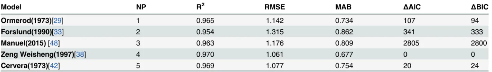
Table 4. Fitting statistics for 5 selected models for detailed analyses.
Model NP R2 RMSE MAB ΔAIC ΔBIC
Ormerod(1973)[29] 1 0.965 1.142 0.734 107 94
Forslund(1990)[33] 2 0.954 1.315 0.862 341 333
Manuel(2015)[48] 3 0.963 1.176 0.809 2805 2800
Zeng Weisheng(1997)[38] 4 0.970 1.061 0.677 0 0
Cervera(1973)[42] 5 0.969 1.077 0.754 20 24
Note:ΔAIC andΔBIC represent the difference in AIC or BIC as compared with the best equation. The best model is the one presenting the lowestΔAIC or
ΔBIC.
whereσ2is within-tree residual variance, Diis the ith tree diameter at breast height,δ1andδ2is
variance—covariance parameters for random effects.
Evaluation of the prediction strategies based on the best model
Based on the random parameters for all developing trees, which were estimated to predict the volume, the MAB was 0.0108, the R2was 0.9981, and the RMSE was 0.0119.
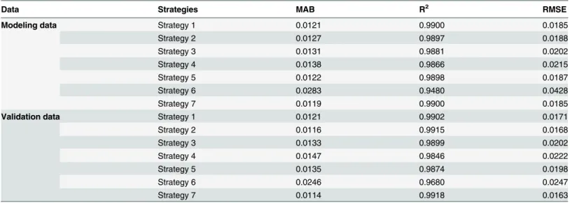
Strategie 7 calculated the total height of 3, 6 and 9 trees in the largest, smallest and medium-size categories and obtained the smallest MAB (0.0119), an adjusted coefficient of determina-tion R2of 0.9900, and the smallest RMSE, of 0.0185. Strategies 1, 2 and 5 produced similar val-ues for MAB, RMSE, and R2. Strategie 2 calculated the fixed part of a mixed-effect model better than strategie 1, which calculated a fixed-parameter model with MAB 0.0006 m3, R20.0003, and RMSE 0.0003 m3, and strategie 5, which calculated the total height of the 1–10 smallest trees with MAB 0.0001 m3, R20.0002, and RMSE 0.0002 m3. Strategie 3, which calculated the total height of 1–10 randomly selected trees, and strategie 4, which calculated the total height of the 1–10 largest trees, had low accuracy. The worst strategie is strategie 6, which calculated Fig 3. Relationship between the aboveground height, total height, diameter at breast height and the parameter b0.
doi:10.1371/journal.pone.0140095.g003
Table 5. Comparison between the new taper model and the best taper model.
Models R2 RMSE MAB NP
(1) 0.970 1.065 0.677 4
d2¼D2 ðH hÞ ðH 1:3Þ
ðb1þb2h0:007Þ 0.971 1.048 0.675 2
the total height of 1–10 medium-size trees; its R2is only 0.9480, which is substantially poorer than the best R2of 0.0420.
Discussion
This paper provides a thorough generalization of many published taper equations with fewer than 5 parameters. The accuracy of the models in an independent data set shows that the sam-ple size and design were sufficient [50–51]. In general, taper models with more parameters pro-duce better fit than those with fewer parameters. However, we found that the models with fewer parameters performed better than certain models with more parameters; for example,
the equationd2¼D2 ðH hÞ ðH 1:3Þ
ððb1þbÞþb2h0:007Þ
with two parameters performs better thanEq 1with
four parameters or the equations withfive parameters (Table 6). We also know that including too many parameters in nonlinear mixed-effect models is not good for convergence. Thus, under some conditions, the modified model in this paper may be better than other models with more parameters forCunninghamia lanceolatain Fujian Province, China, or for other trees worldwide.
In the taperModel (1), in parameter b0, a larger height corresponds to a smaller b0. Thus, we choose parameter h as the only parameter in b0 to modify the taper, and the validation pro-cess demonstrates that this method is accurate.
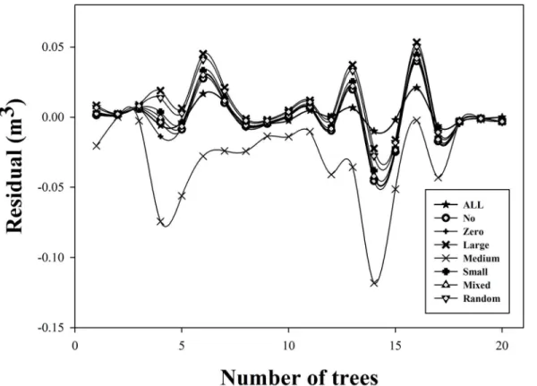
Several strategies were compared in this study using the model that was considered the best based on ease of convergence and a small number of parameters. Seven prediction strategies are readily used in forestry practice. Strategie 7, which calculates the total height of 3, 6 and 9 trees in the largest, smallest and medium-size categories, respectively, has the best accuracy (Fig 4), which suggests that the largest and smallest trees show substantial differences in stem form. The numbers for the 3, 6 and 9 trees large, small and medium-size categories form a nearly normal distribution. Thus, computing the random-effect parameters of the largest, smallest, and medium-size trees clearly improves the predictive accuracy. The calibrated taper model allows the acquisition of accurate results with a notably small sampling effort, which makes this method extremely effective and useful (Table 7).
Strategie 1, which calculates a fixed-parameter model, and strategie 2, which calculates the fixed part of a mixed-effect model, have good accuracy with nearly random parameters for all developing trees. In other words, when the purpose of the model is prediction and calibration data are not available, strategies 1 and 2 should be used based on the best taper model that was modified in this paper. These results are similar to those of de-Miguel [4,23].
Strategies 6 and 4 calculate the heights of medium-size selected trees (total height of 1–10 medium-size trees to calculate the parameters) and the largest selected trees (total height of 1–10 largest trees to calculate the parameters), respectively. Based on the bias results (Fig 5), we find that strategies 6 and 4 were the poorest approaches: strategie 4, using the largest trees, has
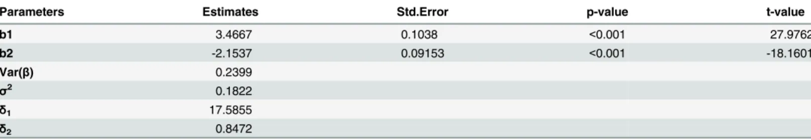
Table 6. Estimates of two fixed regression coefficients and the random parameter of the mixed-effect model based on the modified taper model.
Parameters Estimates Std.Error p-value t-value
b1 3.4667 0.1038 <0.001 27.9762
b2 -2.1537 0.09153 <0.001 -18.1601
Var(β) 0.2399
σ2 0.1822
δ1 17.5855
δ2 0.8472
a larger bias than the other strategies, and strategie 6, using medium-size trees, has a smaller bias than the other strategies. In forest practice, the sample trees are usually average trees, and the medium-size trees are always the average tree in a sample plot (medium-size tree as analytic trees with the average diameter at breast height). Similarly, the largest trees are always the dom-inant tree in a sample plot, in which they have the largest DBH or total height. Thus, when we Fig 4. Predictions with the Xia’s volume equations and strategie 7 vs. the measured stem volume [49].
doi:10.1371/journal.pone.0140095.g004
Table 7. Results of model evaluation and validation in volume prediction (m3) according to different prediction strategies without calibration.
Data Strategies MAB R2 RMSE
Modeling data Strategy 1 0.0121 0.9900 0.0185
Strategy 2 0.0127 0.9897 0.0188
Strategy 3 0.0131 0.9881 0.0202
Strategy 4 0.0138 0.9866 0.0215
Strategy 5 0.0122 0.9898 0.0187
Strategy 6 0.0283 0.9480 0.0428
Strategy 7 0.0119 0.9900 0.0185
Validation data Strategy 1 0.0121 0.9902 0.0171
Strategy 2 0.0116 0.9915 0.0168
Strategy 3 0.0133 0.9899 0.0202
Strategy 4 0.0147 0.9846 0.0222
Strategy 5 0.0135 0.9874 0.0198
Strategy 6 0.0246 0.9680 0.0247
Strategy 7 0.0114 0.9918 0.0163
use the NLME to predict the volume in a forest stand, we cannot use the average trees or domi-nant trees to calculate the random parameter to estimate the stand volume; those approaches would produce the lowest accuracy.
Conclusion
The taper model developed in this paper is the best taper model for describing stands of Cun-ninghamia lanceolata. It has the advantage of easy convergence and simple structure, is a useful tool for predicting the volume ofCunninghamia lanceolataand may also be useful for analyz-ing the taper of other trees worldwide.
In forest practice, when we use the NLME to estimate the stand volume, we cannot use the average trees or dominant trees to calculate the random parameter as the stand random param-eter. We should sample some small trees in a mixed approach (strategie 7) to obtain good accuracy.
The results of this study show that when the purpose of the taper model is prediction and calibration data are not available, fixed-effect (with no random parameter) or mixed-effect (random parameter is 0) models should be used. However, because calibration may sometimes be performed for some but not all types of wood, strategie 7 is one of the best strategies to improve the volume prediction accuracy at tree level. This strategie helps the user make the best selection in random-effects calculation for practical applications and scenarios. Fig 5. Residuals for the calibrated model with different tree sampling designs and sampling sizes to calculate the random parameters.Note: All: calculate all trees; no: with no random parameter; zero: random parameter is 0; large: largest trees; medium: medium-size trees, small: smallest trees; mixed: a mix of large, medium and small trees; random: randomly selected trees.
Supporting Information
S1 Text. Minimal data set of 35 cut trees. (DOCX)
S2 Text. R code for model analysis. (DOCX)
Acknowledgments
The authors thanks for Reviews’comments and suggestions. And thanks for Yunfei Dong, Mukete Beckline, Ling Chen, Fang Jing and other researchers in major of Forest Management in Beijing Forestry University for this study. Total expense of field investigation was borne by the project of forestry science and technology research (No.2012-07), the National Technology Extension Fund of Forestry ([2014]26).
Author Contributions
Conceived and designed the experiments: MG SY. Performed the experiments: MG. Analyzed the data: MG XH Sd-M. Contributed reagents/materials/analysis tools: XH Sd-M. Wrote the paper: MG SY. Revised the manuscript: MG Sd-M SY.
References
1. Flórez V, Valenzuela C, Acuña E, Cancino J. Combining Taper and Basic Wood Density Equations for Estimating Stem Biomass of the Populus X Canadensis I–88 Variety. Bosque. 2014; 35(1): 89–100.
2. Hjelm B. Stem Taper Equations for Poplars Growing On Farmland in Sweden. Journal of Forestry Research. 2013; 24(1):15–22.
3. Kozak A. My Last Words On Taper Equations. Forest Chron. 2004; 80:507–515.
4. De-Miguel S, Mehtatalo L, Shater Z. Evaluating Marginal and Conditional Predictions of Taper Models in the Absence of Calibration Data. Canadian Journal of Forest Research, 2012; 42(7):1383–1394.
5. Von Gadow K, Hui GY. Modelling Forest Development (Page 96 et Sqq). Kluwer Academic Publishers. 1999.
6. Hussein KA, Schmidt M, Kotzé H, Von Gadow K. Parameter-Parsimonious Taper Functions for Describing Stem Profiles. Scientia Silvae Sinicae.2008; 44 (6): 1–8.
7. Diéguez-Aranda U, Castedo-Dorado F, Álvarez-González JG, Rojo A. Compatible Taper Function for
Scots Pine Plantations in Northwestern Spain. Can. J. For. Res. 2006; 36(5): 1190–1205.
8. Menéndez-Miguélez M, Canga E, Álvarez-Álvarez P, Majada J. Stem Taper Function for Sweet Chest-nut (Castanea Sativa Mill.) Coppice Stands in Northwest Spain. Ann Forest Sci. 2014; 71(7):761–770.
9. Lumbres RIC, Lee YJ, Choi HS, Kim SY, Jang MN, Abino AC, et al. Comparative Analysis of Four Stem Taper Models for Quercus Glauca in Mount Halla, Jeju Island, South Korea. Journal of Mountain Sci-ence. 2014; 11(2):442–448.
10. Ung CH, Guo XJ, Fortin M. Canadian National Taper Models. The Forestry Chronicle. 2013; 89 (2):211–224.
11. Rodriguez F, Lizarralde I, Fernández-Landa A, Condes S. Non-Destructive Measurement Techniques for Taper Equation Development: A Study Case in the Spanish Northern Iberian Range. European Journal of Forest Research. 2014; 133(2):213–223.
12. Jiang LC, Liu RL. Segmented Taper Equations with Crown Ratio and Stand Density for Dahurian Larch (Larix Gmelinii) in Northeastern China. Journal of Forestry Research. 2011; 22(3):347–352.
13. Kozak A. Effects of Multicollinearity and Autocorrelation On the Variable Exponent Taper Functions.
Can. J. For. Res. 1997; 27(5): 619–629.
14. Lejeune G, Ung C, Fortin M, Guo XJ, Lambert MC, Ruel JC. A Simple Stem Taper Model with Mixed Effects for Boreal Black Spruce. European Journal of Forest Research. 2009; 128(5):505–513.
16. Trincado G, Burkhart HE. A Generalized Approach for Modelling and Localizing Stem Profiles Curves. For. Sci. 2006; 52: 670–682.
17. Brooks JR, Jiang LC, Ozçelik R. Compatible Stem Volume and Taper Equations for Brutian Pine, Cedar of Lebanon,and Cilicica Fir in Turkey. For. Ecol. Manage. 2008; 256(1–2): 147–151.
18. Leites LP, Robinson AP. Improving Taper Equations of Loblolly Pine with Crown Dimensions in a
Mixed-Effects Modeling Framework. For. Sci. 2004; 50(2): 204–212.
19. Cao QV. Calibrating a Segmented Taper Equation with Two Diameter Measurements. South. J. Appl. For. 2009; 33(2): 58–61.
20. Özçelik R, Brooks JR, Jiang LC. Modeling Stem Profile of Lebanon Cedar, Brutian Pine, and Cilicica Fir in Southern Turkey Using Nonlinear Mixed-Effects Models. Eur. J. For. Res. 2011; 130(4): 613–621.
21. Cao QV, Wang J. Calibrating Fixed- and Mixed-Effects Taper Equations. For. Ecol. Manage. 2011; 262
(4): 671–673.
22. Max TA, Burkhart HE. Segmented Polynomial Regression Applied to Taper Equations. For. Sci. 1976;
22:283–289.
23. De-Miguel S, Guzmán G, Pukkala T. A Comparison of Fixed- and Mixed-Effects Modeling in Tree Growth and Yield Prediction of an Indigenous Neotropical Species (Centrolobium Tomentosum) in a Plantation System. Forest Ecology and Management. 2013; 291:249–258.
24. Crecente-Campo F, Tome M, Soares P, Diéguez-Aranda U. A Generalized Nonlinear Mixed-Effects Height—Diameter Model for Eucalyptus Globulus L. In Northwestern Spain. Forest Ecology and Man-agement. 2010; 259:943–952.
25. Robert BO, David B, Caryanne V. Development of a System of Taper and Volume Tables for Red Alder. For. Sci. 1968; 14: 339–350.
26. Xu H., Sun YJ, Wang XJ, Li Y. Height-Diameter Models of Chinese Fir (Cunninghamia Lanceolata) Based On Nonlinear Mixed Effects Models in Southeast China. Advance Journal of Food Science and Technology.2014; 6(4)445–452.
27. Rojo A, Perales X, Sanchez-Rodriguez F, Alvarez-Gonzalez JG, von Gadow K. Stem Taper Functions for Maritime Pine (Pinus Pinaster Ait.) in Galicia (Northwestern Spain)J. European Journal of Forest Research,2005, 124(3):177–186.
28. Zhang JG, Duan AG, Sun HG. Self-Thinning and Growth Modeling for Even-Aged Chinese Fir
(Cun-ninghamia Lanceolata (Lamb Hook.)Stands. Science Press, Beijing. 2011.
29. Prodan M, Peters R, Cox F. Mensura Forestal.IICA-BMZ/GTZ, San José, Costa Rica. 1997.
30. Gregoire TG, Schabenberger O, Kong F. Prediction From an Integrated Regression Equation: A For-estry Application.Biometrics, 2000; 56(2): 414–419. PMID:10877298
31. Kozak A, Munro DD, Smith JHG. Taper Functions and their Application in Forest Inventory. The For-estry Chronicle. 1969; 45(4):278–283.
32. Ormerod DW. A Simple Bole Model. Forest Chronicle. 1973; 49:136–138.
33. Demaerschalk JP. Converting Volume Equations to Compatible Taper Equations. For Sci. 1972; 18 (3):241–245.
34. Biging Greg S. Taper Equations for Second-Growth Mixed Conifers of Nothern California. For Sci,1984; 30(4):1103–1117.
35. Newberry JD, Burkhart HE. Variable Form Stem Profile Models for Loblolly Pine. Can J for Res. 1986; 16:109–114.
36. Reed DD, Green EJ. Compatible Stem Taper and Volume Ratio Equations. For Sci. 1984; 30(4):977– 990.
37. Forslund RR. The Power Function as a Simple Stem Profile Examination Tool. Can J for Res. 1990; 21:193–198.
38. Coffre M Modelos Fustales. Tesis Ing. For. Universidad Austral De Chile. 1982; 44.
39. Real PL, Moore JA. An Individual Tree System for Douglas Fir in the Inland North-West. USDA Forestry
Service General Technical Report NC–120, 1986;P1037–1044.
40. Manuel AR, Ulises DA, Francisco RP, Carlos ALS, Elena CL, Asunción CO, et al. Modelling and Local-izing a Stem Taper Function forPinus Radiata in Spain[J]. Canadian Journal of Forest Research. 2015, 45(6): 647–658.
41. Bennett FA, Swindel BF. Taper Curves for Planted Slash Pine. USDA Forest Service, Southeastern Forest Experiment Station, Asheville, N.C., Research Note 179.1972.
43. Zeng WS, Liao ZY. The Study of Taper Model. Forest Science. 1997; 33(2):127–132.(In Chinese).
44. Sharma M, Oderwald R. Dimensionally Compatible Volume and Taper. Can J for Res. 2001; 31:797– 803.
45. Goulding C, Murray J. Polynomial Taper Equations that are Compatible with Tree Volume Equations. New Zealand J for Sci.1976; 5:313–322.
46. Lee WK, Seo JH, Son YM, Lee KH, Von Gadow K. Modeling Stem Profiles for Pinus Densiflora in Korea. For Ecol Manag.2003; 172:69–77.
47. Cervera J El á Rea Basimé Trica Reducida, El Volumen Reducido Y El Perfil. Montes. 1973; 174:415– 418.
48. Pinheiro J, Bates D. Mixed Effects Models in S and S-Plus. Spring-Verlag, New York. 2000. 49. Xia ZS, Zeng WS, Zhu S, Luo HZ. Construction of Tree Volume Equations for Chinese Fir Plantations
in Guizhou Province, Southwestern China. For. Sci. Prac., 2013; 15(3):179–185.
50. Kitikidou K, Chatzilazarou G. Estimating the Sample Size for Fitting Taper Equations. J. For. Sci. 2008; 54(4): 176–182.
51. Newton PF, Sharma M. Evaluation of Sampling Design On Taper Equation Performance in