www.ann-geophys.net/24/1317/2006/ © European Geosciences Union 2006
Annales
Geophysicae
Observations and modeling of post-midnight uplifts near the
magnetic equator
M. J. Nicolls1, M. C. Kelley1, M. N. Vlasov1, Y. Sahai2, J. L. Chau3, D. L. Hysell4, P. R. Fagundes2, F. Becker-Guedes2, and W. L. C. Lima5
1School of Electrical and Computer Engineering, Cornell University, Ithaca, New York, USA
2Laboratorio de Fisica e Astronomia, Universidade do Vale do Paraiba (UNIVAP), Sao Jose dos Campos, SP, Brazil 3Radio Observatorio de Jicamarca, Instituto Geofisico del Peru, Lima, Peru
4Department of Earth and Atmospheric Sciences, Cornell University, Ithaca, New York
5Centro Universitario Luterano de Palmas (CEULP), Universidade Luterana do Brazil (ULBRA), Palmas, TO, Brazil
Received: 4 August 2005 – Revised: 1 February 2006 – Accepted: 21 April 2006 – Published: 3 July 2006 Part of Special Issue “The 11th International Symposium on Equatorial Aeronomy (ISEA-11), Taipei, May 2005”
Abstract. We report here on post-midnight uplifts near the magnetic equator. We present observational evidence from digital ionosondes in Brazil, a digisonde in Peru, and other measurements at the Jicamarca Radio Observatory that show that these uplifts occur fairly regularly in the post-midnight period, raising the ionosphere by tens of kilometers in the most mild events and by over a hundred kilometers in the most severe events. We show that in general the uplifts are not the result of a zonal electric field reversal, and demon-strate instead that the uplifts occur as the ionospheric re-sponse to a decreasing westward electric field in conjunction with sufficient recombination and plasma flux. The decreas-ing westward electric field may be caused by a change in the wind system related to the midnight pressure bulge, which is associated with the midnight temperature maximum. In or-der to agree with observations from Jicamarca and Palmas, Brazil, it is shown that there must exist sufficient horizon-tal plasma flux associated with the pressure bulge. In ad-dition, we show that the uplifts may be correlated with a secondary maximum in the spread-F occurrence rate in the post-midnight period. The uplifts are strongly seasonally de-pendent, presumably according to the seasonal dependence of the midnight pressure bulge, which leads to the necessary small westward field in the post-midnight period during cer-tain seasons. We also discuss the enhancement of the uplifts associated with increased geomagnetic activity, which may be related to disturbance dynamo winds. Finally, we show that it is possible using simple numerical techniques to esti-mate the horizontal plasma flux and the vertical drift velocity from electron density measurements in the post-midnight pe-riod.
Correspondence to:M. J. Nicolls
Keywords. Ionosphere (Equatorial ionosphere; Modeling and forecasting; Ionospheric disturbances)
1 Introduction
It is well-known that the height of theF-region ionosphere is the major parameter in controlling the onset of equatorial spreadF (ESF) (Farley et al., 1970). This relationship is due to the fact that the growth rate for the generalized Rayleigh-Taylor instability is inversely proportional to the ion-neutral collision frequency, which decreases exponentially with alti-tude (Kelley et al., 1979a). A second term in the growth rate depends on the eastward electric field, which is destabiliz-ing afterF-region sunset and stabilizing during the night as dictated by the nominalF-region electric field driven by the dynamo wind systems (e.g., Fejer et al., 1979).
Fig. 1.Virtual height contours as measured in Sao Jose dos Campos and Palmas, Brazil, on 1 and 2 October 2002.
In this paper, we discuss what could be a source for a secondary post-midnight maximum in the ESF occurrence rate that has been reported by MacDougall et al. (1998), who observed eastwardly convecting irregularity patches co-incident with “bottomside bulges”. Such a maximum was also observed by Hysell and Burcham (2002). We show ob-servational evidence from digital ionosondes in Brazil and a digisonde at Jicamarca, Peru for what we term “post-midnight uplifts”, which may be the same phenomenon as the bottomside bulges. The term “uplift” refers to the ob-served increase in height of theF-region ionosphere. We note here that such a “lifting” does not say anything about the sign of the electric field because of other terms in the continuity equation.
We explain these uplifts in terms of phenomena associated with the midnight pressure bulge (e.g., Fesen, 1996). This pressure bulge is associated with a convergence of merid-ional thermospheric winds near the equator (e.g., Faivre
et al., 2006), which produce interesting features such as the midnight temperature maximum (e.g., Sastri et al., 1994) and the midnight density maximum (e.g., Arduini et al., 1997).
150 200 250 300 350 400 450
Altitude (km)
Jicamarca: October 1−2, 2002
Time (UT,LT+5)
Altitude (km)
5 6 7 8 9 10 11 12 13 14 15
200 400 600 800 1000 1200 1400 1600 1800
Fig. 2.Isodensity contours as measured by the Jicamarca digisonde on 2 October 2002 and measurements of coherent backscatter from the JULIA radar at Jicamarca.
2 Observational evidence
On the geomagnetically disturbed night of 1–2 October 2002, a series of large-scale traveling ionospheric disturbances (LSTIDs) propagated from high to low latitudes, causing large fluctuations in NmF2 and hmF2 as observed at the Arecibo Observatory (18.34◦N, 66.75◦W, dip 46◦). This event has been reported and discussed by Nicolls et al. (2004) and Vlasov et al. (2005). Nicolls and Kelley (2005) also showed that the final LSTID before sunrise caused the Arecibo ionosphere to rise to over 450 km, and subsequently led to plasma structuring presumably due to some sort of in-stability mechanism.
In Fig. 1 we show observations from two digital ionoson-des in Brazil on this interesting night along with the previous night (1 October). The panels are iso-density contours from Sao Jose dos Campos (23.2◦S, 45.9◦W, dip –32◦) and Pal-mas (10.2◦S, 48.2◦W, dip –11◦) in Brazil. On 2 October at the low-latitude station (Sao Jose dos Campos – SJC) we see oscillations in the height of the ionosphere induced by the propagating LSTID. These observations are very simi-lar to those observed at Arecibo and are caused by the TID neutral winds coupled with a sufficient dip angle. At the equatorial station (Palmas–PAL) on this night we do not see these oscillations because of the much smaller dip angle. In-stead, we see a large uplift of over 100 km between about
05:00 and 09:00 UT (02:00–06:00 LT). On the previous night (30 September–1 October), we do not see the oscillations as-sociated with the LSTID. However, we do see an uplift at the equatorial station. It should be noted that on both 1 Oc-tober and 2 OcOc-tober there was significant auroral electrojet (AE) activity, which could be a major cause of these height increases through disturbance electric fields. We discuss this possibility later.
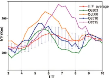
Fig. 3.Virtual height of theFpeak for several days in October 2002 along with the monthly average as measured at Palmas, Brazil.
The event on the night of 1–2 October 2002 was anoma-lous and coincident with a geomagnetic storm (Nicolls et al., 2004). However, the uplifts occur fairly regularly in the equatorial ionosphere with no strong correlation to Kp. This is illustrated by the fact that the uplifts occurred on the pre-vious night of 30 September–1 October as well, which was a much quieter night (see Fig. 1). Figure 3 shows the vir-tual height of theF peak for several other days in October along with the monthly average with errorbars correspond-ing to the standard deviation. We should note that while rel-atively quiet, these nights were all disturbed to some degree, as dictated by the auroral electrojet indices, especially sev-eral hours preceding the layer uplift. The quietest of the days, October 15, was preceded by weak AE activity on the previ-ous day. We discuss the potential influence of auroral activity later, however we should emphasize that the uplifts appear to be a quiet-time phenomenon but strongly sensitive to auroral activity. The monthly average indicates an average uplift of about 50 km in the month of October 2002, with significant variations on that curve as noted by the example days.
The averages for many months between 2002 and 2004 are shown in Fig. 4. We have binned them here in terms of sea-son into equinox and winter / summer, and we showfoF2 on the bottom andh′F data on the top (the virtual height of the F peak). In the virtual height data, the uplifts are evident at equinox, and are especially pronounced during a couple of months (dark blue and orange curves) which correspond to October of 2003 and October of 2002, respectively. The up-lifts are evident, however, in most of the equinox curves. In the winter / summer curves, the uplifts are not present except for a weak one in June of 2002 (red curve). The signature of the uplifts can also be seen in thefoF2 data for equinox. After midnight, the density decreases relatively constantly at a rate of about 2 MHz per hour as a signature of the reverse fountain effect. However, during the time of the uplifts, a
slowing of the density decrease is observed to about 1 MHz per hour, which should be expected. This is a result of a de-crease in the recombination rate as the ionosphere rises. The seasonal variation of the uplifts and the role of the reverse fountain effect will be discussed later.
A similar plot as Fig. 4 using the Jicamarca digisonde is shown in Fig. 5. The data plotted here are from 2002, and each curve is a monthly average with the blue lines rep-resenting equinox months and the black lines reprep-resenting winter / summer months. The uplifts are again evident in the post-midnight period (before 10:00 UT) in the equinox months. The magnitude of the average uplifts are not much different than those measured at Palmas, despite the near-zero dip angle at Jicamarca. The uplifts should not be con-fused with the significant rise inh′F after 10:00 UT. This spike inh′F may be caused by the low value offoF2 (near the lowest sounding frequency), which makes it nearly im-possible to determineh′F.
3 Simulations of post-midnight uplifts
In the preceding section, we showed evidence that post-midnight uplifts occur near the magnetic equator on a fairly regular basis. It is well-known that the zonal electric field is westward at night (e.g., Fejer et al., 1979; Kelley, 1989) and there is no reason to think that the zonal electric field is changing sign at this time since such a trend does not show up in long-term averages except perhaps during summer sol-stice, solar minimum periods. We show some case studies later that show that the reversal does not occur. There is a general trend, however, of smaller fields for all seasons dur-ing solar minimum conditions.
The major forces that can drive the ionosphere upwards besides the effect of electric fields are those caused by neutral winds and the horizontal advection of plasma, while recom-bination can cause an apparent motion leading to an uplift as we have defined it (see the introduction). We show in this section that the daily uplifts discussed in Sect. 2 can be ex-plained by including the role of recombination in the conti-nuity equation. Off the equator, winds and diffusion become important and enhance the uplifts. At the equator, there is really no way that winds can directly produce an uplift. For reference, a meridional neutral wind of several hundred me-ters per second would be required to produce a local uplift of 50 km over the course of an hour at the dip latitude of Jicamarca. Such magnitudes are not observed (e.g., Biondi et al., 1999). However, winds can indirectly produce an uplift through meridional advection of plasma, driven by a latitudi-nal gradient in electron density.
3.1 Recombination
180 200 220 240 260 280 300
h‘F (km)
Equinox Data, 2002−2004 Winter/Summer Data, 2002−2004
0 5 10 15 20
0 5 10 15
FoF2 (MHz)
Time (UT, LT+3)
0 5 10 15 20
Time (UT, LT+3)
Fig. 4.Monthly averages offoF2 (left) andh′Fbinned into equinox and winter summer months as measured in Palmas, Brazil.
to illustrate the differences when a finite vertical drift is in-cluded.
For the Northern Hemisphere case, we define theyˆ coor-dinate as parallel to the magnetic field, thezˆcoordinate as perpendicular and north to the magnetic field (vertical at the equator), and thexˆ coordinate as perpendicular and east to the magnetic field, and the vector velocity may be written as v=v⊥+v||=v⊥nzˆ+v⊥exˆ+v||y.ˆ (1)
The continuity equation is, ∂ne
∂t + ∇ ·(nev)=P −L (2)
whereP andLrefer to production and loss terms, respec-tively. The continuity equation may be written as
∂ne
∂t +ne(∇ ·v⊥)+v⊥·(∇ne)+ne ∂v||
∂x +v|| ∂ne
∂x=P−L.(3)
There is no production term at night and the loss term is due to recombination, which is controlled by the reactions that convert O+to molecular ions (which then recombine disso-ciatively). The major reactions in theF-region are thus O++O2→O+2 +O
with reaction rate (St.-Maurice and Torr, 1978) γ1=2.82×10⁻¹¹−7.74×10⁻¹²(Teff/300)+
1.073×10⁻¹²(Teff/300)2−5.17×10−14(Teff/300)3
+9.65×10⁻¹⁶(Teff/300)4cm3s−1 (4)
and
0 5 10 15
2002
FoF2 (MHz)
0 5 10 15 20
200 220 240 260 280 300
Time (UT, LT+5)
h‘F (km)
Time (UT, LT+5)
Altitude (km)
N e contours
7 7.5 8 8.5 9
100 150 200 250 300 350 400 450 500 550 600
0 2 4 6 8
x 105
2 4 6 8 10
x 105
N m
F2 (km)
True Analytical
7 7.5 8 8.5 9200
250 300 350 400
Time (UT, LT+5)
hm
F2 (km)
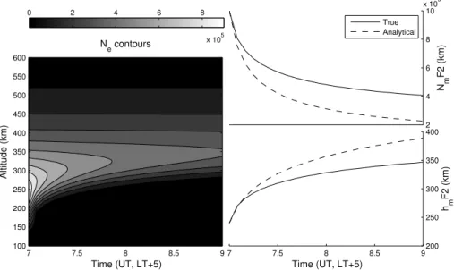
Fig. 6.Electron density as a function of time and altitude for the case of recombination only. The left panel is a contour plot ofne. The right panel isNmF2 (top) andhmF2 (bottom). The solid lines correspond to the values using the recombination rate calculated from MSIS and the dashed lines correspond to the analytical solution of Eqs. (10) and (11).
O++N2→NO++N
with reaction rate (St.-Maurice and Torr, 1978) γ2=1.53×10⁻¹²−5.92×10⁻¹³(Teff/300)+
8.6×10⁻¹⁴(Teff/300)2cm3s−1 (5)
whereTeff=0.667Ti +0.333Tn. The loss term can be writ-ten as L=βne where β is the recombination coefficient, β=γ1[O2] +γ2[N2]. Then,
∂ne
∂t +ne(∇ ·v⊥)+v⊥·(∇ne)+ne ∂v||
∂x +v|| ∂ne
∂x = −βne.(6)
For the case at the magnetic equator, we first make the assumptions that there are no parallel or perpendicular-east gradients in electron density. Then, we are left with the ver-tical velocity (perpendicular-north) term. Assuming no verti-cal velocity, we obtain the simplest continuity equation dom-inated by recombination,
∂ne
∂t = −βne (7)
with solutionne(z, t )=ne0(z)e−β(z)twherene0(z)is the
ini-tial density profile. The effect of recombination in the ab-sence of a vertical drift is to eat away at the bottomside den-sity, increasing the bottomside gradient, decreasing the peak density, and increasing the peak height.
If we let the initial density profile be a Chapman profile, ne0(z)=nm0exp
1 2
1−z−zm0
Hch −
e(zm0−z)/Hch
, (8)
then there is an interesting analytical solution for the peak height and density in the case that β is constant in time and decays exponentially in altitude with the Chapman scale height, i.e.
β(z)=β0e(zm0−z)/Hch (9)
whereβ0is the recombination coefficient at the peak. In this
case, the altitude of the peak and the peak density can be shown to be
zm(t )=zm0+Hchln [1+2β0t] (10)
nm(t )= nm0
√
1+2β0t
(11) wherenm0andzm0correspond to the peak density and
alti-tude of the initial profile.
0 5 10
x 105 200
300 400 500 600
7.05 UT
Altitude (km)
Ne (cm−3)
0 5 10
x 105 200
300 400 500 600
8.11 UT
Ne (cm−3)
0 5 10
x 105 200
300 400 500 600
9.16 UT
Ne (cm−3)
Fig. 7. Profiles of electron density about 1, 2, and 3 h into the simulation for constant downward velocities. The profiles with the lowest densities correspond to the highest downward velocities.
Altitude (km)
0 m/s
200 300 400 500 600
−1 m/s
200 300 400 500 600
−5 m/s
200 300 400 500 600
Altitude (km)
−10 m/s
Time (UT, LT+5)
6 8 10
200 300 400 500 600
−20 m/s
Time (UT, LT+5)
6 8 10
200 300 400 500 600
−30 m/s
Time (UT, LT+5)
6 8 10
200 300 400 500 600
0 2 4 6 8 10 x 105
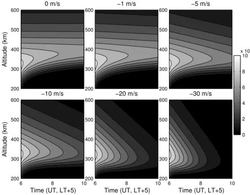
Fig. 8.Contour plots of the electron density for the different values of a constant downward velocity.
3.2 The role of a finite vertical drift
Now, let us consider the role that vertical motion plays in this process. Again at the magnetic equator, neglecting horizontal gradients, the continuity equation, Eq. (6), becomes
∂ne(z, t )
∂t +vz(z, t )
∂ne(z, t )
∂z +ne(z, t )
∂vz(z, t )
∂z =
−β(z, t )ne(z, t ) (12)
where we have strictly included the time and altitude depen-dences. vz in Eq. (12) refers to theE×B drift caused by a zonal electric field. Experimental data show thatvz is
ap-proximately uniform with altitude in theFregion in the post-midnight period so that thezdependence can be dropped. Physical analytical solutions to this equation are difficult to obtain, even for a constant drift, and we must turn to a nu-merical approach.
Time (UT, LT+5)
Altitude (km)
0 m/s
6 8 10
200 300 400 500 600
Time (UT, LT+5) 30 m/s
6 8 10
200 300 400 500 600
Time (UT, LT+5) 70 m/s
6 8 10
200 300 400 500 600
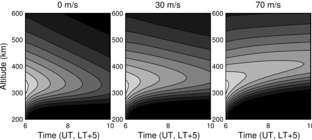
Fig. 9.Contour plots of the electron density for the different values of a constant neutral wind as described in the text. The scale is the same as that in Fig. 8.
corresponding approximately to the profile measured by Ji-camarca at 01:00 LT (06:00 UT) on 16 April 2002. The sim-ulations are run for 4 h. Figure 7 shows profiles at about 1, 2, and 3 h into the simulation, for 6 different values ofvzof 0, –1, –5, –10, –20, and –30 m/s. Figure 8 shows contour plots for each of the cases. The major observation from these curves is that a downward drift leads to a faster decline in density (as one would expect) and at some critical velocity can overcome the uplift induced by recombination.
However, real drifts are a function of time and possibly height. In Sect. 4.1, we will include the effect of a time-dependent velocity.
3.3 Diffusion and winds
Off the equator, in addition to the electric field, ambipolar diffusion, gravity, and neutral winds become important and their role in the vertical velocity must be included in the con-tinuity equation. Equation (12) becomes (e.g., Banks and Kockarts, 1973)
∂ne ∂t +
∂ ∂z
h
−Dasin2I ∂n
e
∂z + ne Hp
+vznecosI −unnesinIcosI
i
= −βne (13)
where Da=kbTp/miνin is the ambipolar diffusion coeffi-cient, I is the magnetic dip angle, Hp=kbTp/mig is the plasma scale height,Tp=Ti+Te,unis the northward neutral wind,νinis the ion-neutral collision frequency, and we have ignored temperature gradients and other neutral motions. It can be expected that diffusion should reduce the magnitude of the uplifts but that neutral winds might enhance them in the case of an equatorward wind. Equatorward winds are ob-served at mid and low latitudes after midnight (e.g., Biondi et al., 1999), although there is an abatement of the wind (e.g., Herrero et al., 1993) associated with the midnight pressure bulge (e.g., Fesen, 1996), which is related to the convergence
of winds near the equator (e.g, Faivre et al., 2006). Some an-alytical solutions to various simplified versions of this conti-nuity equation have been obtained (e.g, Banks and Kockarts, 1973; Duncan, 1956; Dungey, 1956; Martyn, 1956; Rishbeth and Garriott, 1969; Vlasov et al., 2005). However, in general a numerical approach is necessary.
Examples of the behavior with winds, diffusion, and a vertical velocity are shown in Fig. 9 for a constant down-ward drift of 10 m/s and three different values of equatordown-ward wind: 0 m/s, 30 m/s, and 70 m/s. The same initial profile as before was used and the simulation corresponds to the loca-tion of Palmas. At 0 m/s, we see a curve similar to that of Fig. 8 except with slightly increased falling velocity due to the inclusion of diffusion. At 30 m/s, we see a sizable uplift, and at 70 m/s, we see a huge uplift of almost 100 km.
4 Discussion
4.1 Comparison to observations
In the previous section, we showed evidence that recombi-nation induces an apparent uplift at the magnetic equator provided that the downward vertical drift (westward electric field) is sufficiently small. In this subsection, we compare our modeling results to some Jicamarca measurements.
−35 −30 −25 −20 −15 −10 −5 0 5
V z
(m/s)
April 16, 2002
6 6.5 7 7.5 8 8.5 9 9.5 10
310 320 330 340 350 360 370
hmF2 (km)
6 6.5 7 7.5 8 8.5 9 9.5 103
4 5 6 7 8 9 10 x 105
Time (UT,LT+5)
NmF2 (cm
−3
)
Time (UT,LT+5)
Altitude (km)
6 7 8 9 10
200 250 300 350 400 450 500
Time (UT,LT+5)
6 7 8 9 10
200 250 300 350 400 450 500
0 2 4 6 8 10 x 105
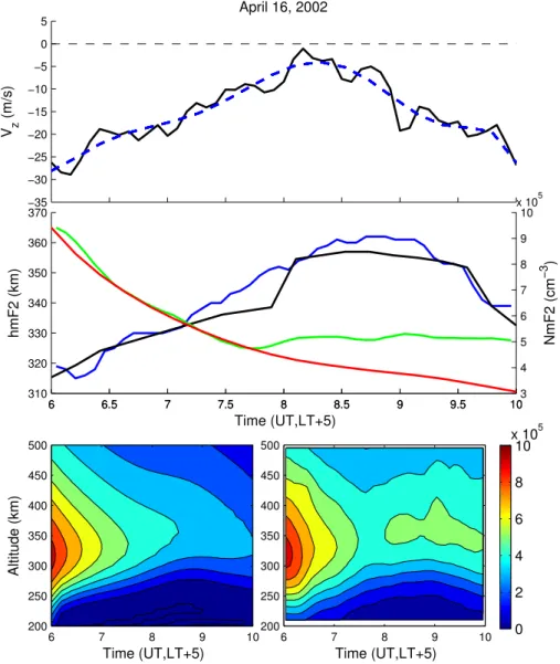
Fig. 10.Data and simulations on 16 April 2002. The top panel is the vertical drift measured by Jicamarca (black solid) and the drift used in the model run (blue dashed). The second panel ishmF2 (measured in blue, modeled in black) andNmF2 (measured in green, modeled in red). The lower panel is a density contour plot of the model (left) and measurements (right).
results are shown in black.NmF2 as measured by Jicamarca is shown as the green line and the model results are shown in red. The lower panels show the modeled and measured densities as a function of height and time. We should note that we have increased the recombination coefficient slightly over the value given using the MSIS parameters for this case to match the observed density decrease.
The vertical drift is observed to decrease in intensity after about 01:00 LT to reach a minimum velocity of near 0 m/s at 03:00 LT, at which point it increases again. This is a charac-teristic that is observed frequently during the uplifts. From the model behavior described in the preceding section, we would expect an uplift at this point and this is exactly what we see. ThehmF2 comparisons show that the model repro-duces the uplift in height quite well. However, in comparing
the densities, we see that up until about 03:00 LT, they agree very well, but after that point, there is a large discrepancy. In fact,NmF2 increases, which can be seen more clearly in the color plot in Fig. 10 where we see a secondary maxi-mum in density in the Jicamarca data. This maximaxi-mum cannot be explained by including only recombination and the one-dimensional plasma motion.
Time (UT,LT+5)
Altitude (km)
6
7
8
9
10
200
250
300
350
400
450
500
Fig. 11. Contour plot of modeled densities including a horizontal plasma flux term as described in the text. The scale is the same as in Fig. 10.
anomaly into the equatorial region, which seems to be the most likely explanation. This advection may be associated with the midnight pressure bulge caused by a convergence of thermospheric winds at low latitudes.
If we subtract the electron density data from the model to obtain the difference, and take the time derivative, we obtain an estimate of the ionization rate necessary for the model to agree with the data (this estimate is only approximate since it ignores recombination and is only calculated at the peak). We find that in this case the rate is close to constant after 02:30 LT with a value near 20–25 cm−3s−1. Such an
ion-ization rate seems too high to be caused by a shear in the vertical drift, implying that plasma flux must be the major source of ionization. Thus, the ionization rate gives us an estimate of the derivative (horizontal gradient) of the plasma flux. The total electron content transported to the equato-rial region for such a horizontal plasma flux can be com-puted as 25 cm−3s−1multiplied by the vertical scale (about 100 km) multiplied by the time scale of the flux. This flux persists for at least 2.5 h, giving a total electron content of about 2.25 TECU (1 TECU = 1012 cm−2) for a gradient in flux of 25 cm−3s−1. This is a reasonable change in the ver-tically integrated electron density observed at at Jicamarca in the post-midnight period, which is typically greater than 10 TECU (e.g., Valladares et al., 2001). We note that our es-timate of the flux and associated TEC increase is probably an upper limit.
Figure 11 shows the results of incorporating the neces-sary horizontal gradient in plasma flux, and we now see very good agreement with the observed density behavior with the modelNmF2 variation matching the data almost exactly. The
6
7
8
9
10
0
5
10
15
20
Time (UT,LT+5)
TEC (TECU)
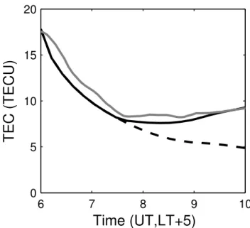
Fig. 12. Total electron content (TEC) from 200 to 450 km for the simulation results presented in Fig. 10 (dashed black) without flux, the simulation results presented in Fig. 11 (solid black) with flux, and the data (gray).
total electron content from 200–450 km for the two simula-tions (with and without flux) and for the data are compared in Fig. 12. The results are in reasonable agreement with the es-timations above. The source of this flux is likely a meridional density gradient.
4.2 Interpretation and variation of uplifts
We have shown that uplifts occur fairly regularly in the equa-torial ionosphere. The uplifts are not caused by a reversal of the zonal electric field, as shown in the case study pre-sented in the previous section and as can be seen by looking at other datasets. However, comparisons to Jicamarca drifts indicate they occur when the vertical drift is small or decreas-ing, which allows recombination to become significant.
18 20 22 24 26 28 30 0
5 10 15 20 25 30
Day of Month
October 2002 Spread F stats, Palmas
18 20 22 24 26 28 30 0
0.2 0.4 0.6 0.8 1
Time (LT, UT−3)
Occ. Prob.
18 20 22 24 26 28 30 0
5 10 15 20 25 30
Day of Month
September 2003 Spread F stats, Palmas
18 20 22 24 26 28 30 0
0.2 0.4 0.6 0.8 1
Time (LT, UT−3)
Occ. Prob.
18 20 22 24 26 28 30 0
5 10 15 20 25 30
Day of Month
October 2003 Spread F stats, Palmas
18 20 22 24 26 28 30 0
0.2 0.4 0.6 0.8 1
Time (LT, UT−3)
Occ. Prob.
18 20 22 24 26 28 30 0
5 10 15 20 25 30
Day of Month
March 2004 Spread F stats, Palmas
18 20 22 24 26 28 30 0
0.2 0.4 0.6 0.8 1
Time (LT, UT−3)
Occ. Prob.
18 20 22 24 26 28 30 0
5 10 15 20 25 30
Day of Month
April 2004 Spread F stats, Palmas
18 20 22 24 26 28 30 0
0.2 0.4 0.6 0.8 1
Time (LT, UT−3)
Occ. Prob.
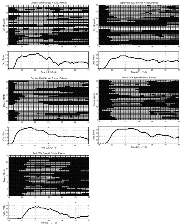
Fig. 13.Spread-Fstatistics at Palmas for several equinox months in 2002, 2003, and 2004. The top panel is the spread-Fstatistics for the entire month as a function of local time and night of month. White corresponds to no data, black corresponds to no spread-F, light gray corresponds to range spreading, and dark gray corresponds to frequency spreading. The lower panel is the averaged probability of occurrence of spread-Ffor the month as a function of local time.
We have mentioned the fact that the magnitude of the uplifts is related to auroral electrojet activity. Storm-time effects can cause variations in the equatorial electric fields through changes in the global wind system, penetrating elec-tric fields (e.g., Nishida et al., 1966; Vasyliunas, 1970; Kel-ley et al., 1979b), and disturbance dynamo winds driven by Joule heating (e.g., Blanc and Richmond, 1980). It is
A recent study by Richmond et al. (2003) has shown that at night the disturbance dynamo tends to drive a current that leads to reductions or reversals in the equatorial zonal elec-tric field. This behavior appears to be consistent with the ob-servations, an uplift and a decrease in the magnitude of the zonal electric field caused by weak auroral electrojet activity. From this explanation, it is clear how enhanced uplifts can occur during times of higher magnetic activity, when the dy-namo disturbance becomes enhanced. As shown in the data from 1–2 October 2002 presented in Sect. 2, enhanced uplifts occur in response to geomagnetic activity. Storm-time ef-fects induced for example by variations in the dynamo wind system could lead to an enhancement of pre-existing irregu-larities, leading to the behavior shown in Fig. 2.
It might be thought that the decrease in magnitude of the zonal electric field can be interpreted in terms of the reverse fountain effect (e.g., King, 1968). The so-called fountain ef-fect is caused in the daytime by the zonal field which drives plasma upwards. The plasma can then fall down the field lines to low-latitudes where it creates the equatorial anoma-lies. At night, the reverse effect can occur. Downward drifts cause decreased plasma pressure on the topside, which can pull plasma from low-latitudes to the equatorial region. When this reverse fountain effect decreases in magnitude due to a decrease in the magnitude of the downward drift, an up-lift can be caused via the mechanisms described already. The inclusion of recombination is essential to reproducing this uplift.
While the effect of the post-midnight wind abatement and the disturbance dynamo can explain the uplifts, it does not explain the density increase that is observed. The interpreta-tion of the density increase in terms of the reverse fountain effect is not satisfactory because at the time of the uplift, the westward electric field is at its weakest and thus the plasma flux caused by the reverse fountain effect is also at its lowest. In order to explain this density increase, we have invoked a horizontal gradient in the meridional plasma flux in Sect. 4.1. This is an inward flux that could be driven by a westward electric field or by a convergence of neutral winds. But, as we have just stated, the observed westward electric field is becoming smaller, which should reduce the plasma flux, not increase it. Thus, the major source of the flux appears to be the convergence of the low-latitude winds associated with the midnight pressure bulge. Other studies have reported a den-sity increase associated with the midnight temperature max-imum or midnight pressure bulge (e.g., Arduini et al., 1997). At this time, it is unclear whether the pressure bulge is sig-nificant enough to drive the gradient in plasma flux that is required for this interpretation.
4.3 Equatorial spread-F
One of the potential implications of the post-midnight up-lifts described in this paper is the generation of a secondary maximum in spread-F occurrence rates. Many papers have
described a secondary maximum in ESF occurrence in the post-midnight period (Abdu et al., 1981, 1983; Fejer et al., 1999; Hysell and Burcham, 2002; MacDougall et al., 1998). During periods of high geomagnetic activity, electric fields can penetrate to low latitudes and cause the equatorial elec-tric field to reverse in the post-midnight period, which is a source of ESF during periods of high geomagnetic activity (Kelley et al., 1979b; Fejer et al., 1999). Hysell and Burcham (2002) divides the pre-sunrise ESF into two categories. The first, as described by Farley et al. (1970) and MacDougall et al. (1998), occur just before sunrise near theF peak. The other may be due to “dead bubbles”. Thus it seems possi-ble that the uplifts described in this paper could contribute to the secondary maximum in ESF occurrence that occurs in the pre-sunrise period.
To illustrate that there is indeed a secondary peak in the ESF occurrence rate, we show Palmas ESF statistics in Fig. 13 for several equinox months. The top panel of each plot shows the statistics for each day of the given month, with range spreading distinguished from frequency spread-ing as described in the caption. The dominant occurrence peak can be seen between 20:00 and 22:00 LT with a de-cline in rate after that point. A secondary peak is seen in all but one of the curves (April 2004), with an occurrence rate of near 40%, most pronounced in October 2002 and March 2004. The peak occurs between 02:00 and 04:00 LT. This corresponds nicely to the time of the uplifts, as depicted in Fig. 4. It is interesting to note that the ESF observed in the late morning is largely of the frequency type. This was also observed by Abdu et al. (1983).
4.4 Extracting velocities from density measurements Recently, Woodman et al. (2006) have compared vertical drifts deduced from digisonde measurements to Jicamarca observations of the vertical drifts. The authors find fair agree-ment at times when strong convection dominates, for exam-ple near the pre-reversal enhancement, but poor agreement at times when production and recombination dominate. The digisonde drifts are deduced from the line-of-sight Doppler velocity, and such measurements have been relatively suc-cessful at high latitudes (e.g., Scali et al., 1995). Woodman et al. (2006) show that the agreement is worst in the post-midnight period, and attribute this disagreement to the rel-ative importance of recombination. There have been other studies on the role of recombination at the equator (e.g., Bit-tencourt and Abdu, 1981).
There exists a very simple method for estimating the drift from the continuity equation. Equation (12) can be solved for the vertical velocity with a horizontal plasma flux term included,
vz= −
βne+∂ne/∂t+∂(nevx)/∂x ∂ne(z, t )/∂z
which is valid for the nighttime equatorial ionosphere. The plasma flux term can be due to either meridional or zonal gra-dients in density. Given bottomside density measurements, one can calculate the time and altitude gradients to estimate the vertical velocity. The plasma flux, of course, is more difficult to measure, although we have demonstrated in this paper a simple method for estimating it given density mea-surements.
It is expected that digisonde drifts on average represent the motion of a constant density contour. Whether the drift is computed from the range rates of the echoes themselves or from the Doppler shifts shouldn’t matter for total reflec-tion. We show an example in Fig. 14 for 16 April 2002. The top panel shows three constant density curves as a function of time from the model case study presented in Fig. 11. The solid line with solid points in the bottom panel corresponds to the expected Doppler velocity that a digisonde would see, which corresponds to the change in height of a constant den-sity contour as a function of time. This was averaged for the three contours in the top panel. The dashed line is the true locity used in the simulation. It is clear that the “Doppler” ve-locity is way off and unphysical – the veve-locity is not even the correct direction. The results are consistent with those pre-sented by Woodman et al. (2006) which show a positive drift during this time period, peaking between 02:00–04:00 LT. The crosses are the velocity estimates using Eq. (14), includ-ing the plasma flux term, which fall exactly on top of the model curve. The small variation is due to errors in esti-mating the gradients. The circles are the calculations using Eq. (14) but neglecting the plasma flux term, since that is in general difficult to estimate. Some error is induced by neglecting the flux, however the estimate is still very good compared to the Doppler result. Thus, it seems possible to estimate the vertical drifts using bottomside density profiles at times when the horizontal plasma flux is not too large. A similar technique was applied by Bertoni (2004) using the SUPIM model.
Note that both the recombination and the time derivative terms are quite important in general and neither should be neglected, at least in the post-midnight time period. During times of high convection (e.g., near the pre-reversal enhance-ment) recombination is negligible and the equation reduces to the motion of a constant density contour, as discussed by Woodman et al. (2006). Using Eq. (14), the Doppler veloc-ities can also be corrected for the effects of recombination and plasma flux in the form,
vz= −vD−
βne+∂(nevx)/∂x ∂ne(z, t )/∂z
(15) wherevDis the measured Doppler velocity.
5 Conclusions
We have shown observational evidence for post-midnight uplifts near the magnetic equator using data from a digital
200 220 240 260 280 300 320
Altitude (km) 2x105 cm−3
3x105 cm−3 4x105 cm−3
6 7 8 9 10
−40 −30 −20 −10 0 10 20 30
V z
(m/s)
Time (UT,LT+5)
Doppler Estimated No flux True
Fig. 14. The top plot shows three constant density contours using the model results presented in Fig. 11. The bottom plot shows the expected digisonde Doppler velocity (solid line with solid points), estimated velocity from density profiles (crosses), estimated veloc-ity ignoring plasma flux (circles), and true velocveloc-ity (dashed line).
ionosonde in Palmas, Brazil and by a digisonde at the Jica-marca Radio Observatory. These uplifts are in general not caused by a reversal in the zonal electric field, but such a reversal would enhance them, which may occur during ac-tive periods. During the time of uplift, the magnitude of the westward electric field decreases (but does not reverse) and recombination causes an apparent lifting of the layer, an increase in hmF2. The change in the westward electric field during these time periods seems to be associated with an abatement of the equatorward neutral wind, induced by the midnight pressure bulge. Enhanced uplifts may be driven by auroral electrojet activity causing the disturbance dynamo to reduce the magnitude of the electric field, as studied by Richmond et al. (2003).
An interpretation of the uplift in terms of the reverse foun-tain effect cannot explain a density increase that is observed during the time of the uplift. In order to explain this increase, we have shown that horizontal plasma flux must be included in our model. These fluxes may be driven by meridional den-sity gradients and a convergence of neutral winds at the equa-tor associated with the midnight density maximum.
in combination with digisonde density measurements could be used to study this flux. Our simple model can be combined with density curves, for example measured by a digisonde, to estimate vertical drifts at the magnetic equator in the post-midnight period.
In addition, we have shown that the uplifts may contribute to a secondary maximum in the equatorial spread-F occur-rence rate that occurs in the post-midnight period. The ex-tent of this maximum appears to agree quite well with the local-time variation of the uplifts.
Acknowledgements. The Jicamarca Radio Observatory is a facility
of the Instituto Geofsico del Peru and is operated with support from the NSF Cooperative Agreement ATM-0432565 through Cornell University. Work at Cornell was sponsored by the Atmospheric Sci-ence Section of the NSF under Grant ATM-0000196. We thank two anonymous reviewers for their careful reading and detailed com-ments which have improved the paper.
Topical Editor M. Pinnock thanks M. Abdu and another referee for their help in evaluating this paper.
References
Abdu, M. A., Batista, I. S., and Bittencourt, J. A.: Some character-istics of spreadFat the magnetic equatorial station Fortaleza, J. Geophys. Res., 86, 6836–6842, 1981.
Abdu, M. A., de Medeiros, R. T., and Nakamura, Y.: Latitudinal and magnetic flux tube extension of the equatorial spread F ir-regularities, J. Geophys. Res., 88, 4861–4868, 1983.
Arduini, C., Laneve, G., and Herrero, F. A.: Local time and altitude variation of equatorial thermosphere midnight density maximum (MDM): San Marco drag balance measurements, Geophys. Res. Lett., 24, 377–380, 1997.
Banks, P. M. and Kockarts, G.: Aeronomy, Part B, Academic Press, Inc., New York, NY, 1973.
Bertoni, F.: Derivas ionsfericas em latitudes equatoriais: Observa-coes e modelagem, Ph.D. thesis, Instituto Nacional de Pesquisas Espaciais, 2004.
Biondi, M. A., Sazykin, S. Y., Fejer, B. G., Meriwether, J. W., and Fesen, C. G.: Equatorial and low latitude thermospheric winds: Measured quiet time variations with season and solar flux from 1980 to 1990, J. Geophys. Res., 104, 17 091–17 106, 1999. Bittencourt, J. A. and Abdu, M. A.: A theoretical comparison
be-tween apparent and real vertical ionization drift velocities in the equatorialFregion, J. Geophys. Res., 86, 2451–2454, 1981. Blanc, M. and Richmond, A. D.: The ionospheric disturbance
dy-namo, J. Geophys. Res., 85, 1669–1686, 1980.
Burnside, R. G., Herrero, F. A., Meriwether, J. W., and Walker, J. C. G.: Optical observations of thermospheric dynamics at Arecibo, J. Geophys. Res., 86, 5532–5540, 1981.
Duncan, R. A.: The behaviour of a Chapman layer in the nightF2
region of the ionosphere, under the influence of gravity, diffu-sion, and attachment, Australian J. Phys., 9, 436–439, 1956. Dungey, J. W.: The effect of ambipolar diffusion in the night-time
Flayer, J. Atmos. Terr. Phys., 9, 90–102, 1956.
Faivre, M., Meriwether, J. W., Fesen, C. G., and Biondi, M. A.: Cli-matology of the midnight temperature maximum phenomenon at Arequipa, Peru, J. Geophys. Res., in press, 2006.
Farley, D. T., Balsley, B. B., Woodman, R. F., and McClure, J. P.: Equatorial spreadF: Implications of VHF radar observations, J. Geophys. Res., 75, 7199–7210, 1970.
Fejer, B. G., Farley, D. T., Woodman, R. F., and Calderon, C.: De-pendence of equatorialF-region vertical drifts on season and so-lar cycle, J. Geophys. Res., 84, 5792–5796, 1979.
Fejer, B. G., Scherliess, L., and de Paula, E. R.: Effects of the verti-cal plasma drift velocity on the generation and evolution of equa-torial spreadF, J. Geophys. Res., 104, 19 859–19 869x, 1999. Feng, Z., Kudeki, E., Woodman, R. F., Chau, J., and Milla, M.:F
region plasma density estimation at Jicamarca using the complex cross-correlation of orthogonal polarized backscatter fields, Ra-dio Sci., 39, RS3015, doi:10.1029/2003RS002963, 2004. Fesen, C. G.: Simulations of the low-latitude midnight temperature
maximum, J. Geophys. Res., 101, 26 863–26 874, 1996. Hedin, A. E.: Extension of the MSIS Thermospheric model into the
middle and lower atmosphere, J. Geophys. Res, 96, 1159–1172, 1991.
Herrero, F. A., Spencer, N. W., and Mayr, H. G.: Thermosphere and F-region plasma dynamics in the equatorial region, Adv. Space Res., 13, 201–220, 1993.
Hysell, D. L. and Burcham, J. D.: JULIA radar studies of equatorial spreadF, J. Geophys. Res., 103, 29 155–29 167, 1998.
Hysell, D. L. and Burcham, J. D.: Long term studies of equatorial spreadF using the JULIA radar at Jicamarca, J. Atmos. Solar-Terr. Phys., 64, 1531–1543, 2002.
Kelley, M. C.: The Earth’s ionosphere: Plasma physics and electro-dynamics, Academic Press, Inc., San Diego, CA, 1989. Kelley, M. C., Baker, K. D., and Ulwick, J. C.: Late time
bar-ium cloud striations and their possible relationship to equatorial spreadF, J. Geophys. Res., 84, 1898–1904, 1979a.
Kelley, M. C., Fejer, B. G., and Gonzales, C. A.: An explanation for anomalous equatorial ionospheric electric fields associated with a northward turning of the interplanetary magnetic field, Geo-phys. Res. Lett., 6, 301–304, 1979b.
Kil, H. and Heelis, R. A.: Global distribution of density irregulari-ties in the equatorial ionosphere, J. Geophys. Res., 103, 407–417, 1998.
King, J. W.: Airglow observations and the decay of the ionospheric equatorial anomaly, J. Atmos. Terr. Phys., 30, 391–397, 1968. Kudeki, E., Bhattacharyya, S., and Woodman, R. F.: A new
ap-proach in incoherent scatterF region E×B drift measurements at Jicamarca, J. Geophys. Res., 104, 28 145–28 162, 1999. MacDougall, J. W., Abdu, M. A., Jayachandran, P. T., Cecile, J. F.,
and Batista, I. S.: Presunrise spreadFat Forteleza, J. Geophys. Res., 103, 23 415–23 425, 1998.
Martyn, D. F.: Processes controlling ionization distribution in the F2 region of the ionosphere, Australian J. Phys., 9, 161–165,
1956.
Nicolls, M. J. and Kelley, M. C.: Strong evidence for gravity wave seeding of an ionospheric plasma instability, Geophys. Res. Lett., 32, L05108, doi:10.1029/2004GL020737, 2005.
Nicolls, M. J., Kelley, M. C., Coster, A. J., Gonz´alez, S. A., and Makela, J. J.: Imaging the structure of a large-scale TID using ISR and TEC data, Geophys. Res. Lett., 31, L09812, doi:10.1029/2004GL019797, 2004.
Richmond, A. D., Peymirat, C., and Roble, R. G.: Long-lasting disturbances in the equatorial ionospheric electric field simulated with a coupled magnetosphere-ionosphere-thermosphere model, J. Geophys. Res., 108, 1118, doi:10.1029/2002JA009758, 2003. Rishbeth, H. and Garriott, O. K.: Introduction to ionospheric
physics, Academic Press, Inc., New York, NY, 1969.
Sastri, J. H., Rao, H. N., Somayajulu, V. V., and Chandra, H.: Ther-mospheric meridional neutral winds associated with equatorial midnight temperature maximum (MTM), Geophys. Res. Lett., 21, 825–828, 1994.
Scali, J. L., Reinisch, B. W., Heinselman, C. J., and Bullet, T.: Co-ordinated digisonde and incoherent scatter radarF region drift measurements at Sondre Stromfjord, Radio Sci., 30, 1481–1498, 1995.
St.-Maurice, J. P. and Torr, D. G.: Nonthermal rate coefficients in the ionosphere: The reactions of O+with N2, O2, and NO, J.
Geophys. Res., 83, 969–977, 1978.
Valladares, C. E., Basu, S., Groves, K., Hagan, M. P., Hysell, D., Mazzella, A. J., and Sheehan, R. E.: Measurement of the lat-itudinal distributions of total electron content during equatorial spreadFevents, J. Geophys. Res., 106, 29 133–29 152, 2001. Vasyliunas, V. M.: Mathematical models of magnetospheric
con-vection and its coupling to the ionosphere, in Particles and Fields in the Magnetosphere, edited by: McCormac, M., D. Reidel, Nor-well, MA, p. 60, 1970.
Vlasov, M. N., Nicolls, M. J., Kelley, M. C., Smith, S. M., Aponte, N., and Gonz´alez, S. A.: Modeling of airglow and ionospheric parameters at Arecibo during quiet and disturbed periods in October 2002, J. Geophys. Res., 110, A07303, doi:10.1029/2005JA011074, 2005.