Relation of zonal plasma drift and wind in the equatorial F region as derived from CHAMP observations

(1)

www.ann-geophys.net/31/1035/2013/ doi:10.5194/angeo-31-1035-2013

Annales

Geophysicae

Geoscientiic

Relation of zonal plasma drift and wind in the equatorial F region as

derived from CHAMP observations

J. Park and H. L ¨uhr

GFZ, German Research Centre for Geosciences, Potsdam, Germany Correspondence to:J. Park ([email protected])

Received: 7 January 2013 – Revised: 15 May 2013 – Accepted: 15 May 2013 – Published: 12 June 2013

Abstract. In this paper we estimate zonal plasma drift in the equatorial ionospheric F region without counting on ion drift meters. From June 2001 to June 2004 zonal plasma drift velocity is estimated from electron, neutral, and mag-netic field observations of Challenging Mini-satellite Pay-load (CHAMP) in the 09:00–20:00 LT sector. The estimated velocities are validated against ion drift measurements by the Republic of China Satellite-1/Ionospheric Plasma and Electrodynamics Instrument (ROCSAT-1/IPEI) during the same period. The correlation between the CHAMP (altitude

∼400 km) estimates and ROCSAT-1 (altitude∼600 km) ob-servations is reasonably high (R_≈0.8). The slope of the linear regression is close to unity. However, the maximum westward drift and the westward-to-eastward reversal occur earlier for CHAMP estimates than for ROCSAT-1 measure-ments. In the equatorial F region both zonal wind and plasma drift have the same direction. Both generate vertical currents but with opposite signs. The wind effect (F region wind dy-namo) is generally larger in magnitude than the plasma drift effect (Pedersen current generated by vertical E field), thus determining the direction of the F region vertical current. Keywords. Ionosphere (Equatorial ionosphere)

1 Introduction

The ionospheric F region is an important medium for radio communication. Among a variety of parameters characteriz-ing the F region, the plasma density is one of the most es-sential parameters because it determines the reflection height of various radio waves (e.g. Chen et al., 2011), affects the phase delay of wave signals (e.g. Jee et al., 2004; Noja et al., 2013), and disturbs communication links (e.g. Basu et al., 1988, 2001; Nishioka et al., 2011; Manju et al., 2011).

Plasma density in the ionospheric F region is controlled not only by local ionization/loss processes, but also by plasma transport. Therefore, the climatology of the F region plasma drift has gained significant attention in ionospheric science. Especially, the vertical drift has direct control over the F layer height, which affects the recombination rate. The majority of previous studies about F region plasma transport have fo-cused on the vertical drift (e.g. Sastri, 1996; Scherliess and Fejer, 1999; Hartman and Heelis, 2007; Kil et al., 2007; Fe-jer et al., 2008; Stolle et al., 2008, to name only a few). The horizontal drift (e.g. Coley et al., 1994; Maynard et al., 1995; Fejer et al., 2005; Pacheco et al., 2011), on the other hand, has been given relatively less attention. Zonal drift of F re-gion plasma is generally westward (eastward) during day-time (nightday-time) (e.g. Fejer et al., 2005, Fig. 1). As the east-ward drift speed at low latitudes is generally stronger than the westward one, the daily average of the zonal drift results in net eastward drift: the so-called super-rotation (e.g. Pacheco et al., 2011). As the latitudes get lower, the super-rotation becomes stronger. The magnitude of zonal drift speed on the dayside (nightside) exhibits weak (strong) positive correla-tion with the solarF10.7index (e.g. Fejer et al., 2005, Fig. 2).

The zonal drift depends on longitude as well as on latitude (e.g. Pacheco et al., 2011).

(2)

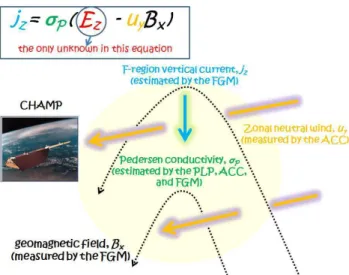
Fig. 1.Schematic diagram of the procedure for estimating zonal plasma drift velocity from CHAMP measurements.

In this paper we estimate zonal plasma drift in the equa-torial ionospheric F region indirectly from the Challenging Mini-Satellite Payload (CHAMP) measurements. We also make direct comparisons between zonal wind and plasma drift in the low-latitude F region. Furthermore, we assess the influence of these two components on the vertical current flowing in the equatorial F region. In Sect. 2 the instruments and the derivation methods are described. The estimated ve-locities are presented and validated in Sect. 3. The climatol-ogy of the zonal drift is discussed in Sect. 4, and we draw conclusions in Sect. 5.

2 Instrumentation and method

The CHAMP satellite was launched on 15 July 2000 into a circular polar orbit. The orbit altitude was about 450 km right after launch, and decayed slowly until the atmospheric re-entry on 19 September 2010. The orbit inclination an-gle was 87.2◦, so the local time (LT) changed by 12 h over 131 days. The main purpose of CHAMP was precise mea-surement of geomagnetic field, which was performed by the Overhauser Magnetometer (OVM) and the Flux-Gate Magnetometer (FGM). The pre-processed data rate is 1 Hz. The Space Triaxial Accelerometer for Research (STAR or ACC) is the on-board accelerometer, from which we can get information on the neutral mass density and cross-track wind velocity (approximately in the zonal direction in geo-graphic coordinates) every 10 s. The Planar Langmuir Probe (PLP) measures electron density and temperature every 15 s. CHAMP also carried a Digital Ion Drift Meter (DIDM), which could have directly measured the three-dimensional plasma drift velocity. Unfortunately, the DIDM was degraded severely during launch. We can only get relative ion density variation from the DIDM. Below we describe how the zonal

drift speed can be retrieved from the combined observations of the FGM, ACC, and PLP.

The geomagnetic field vectors observed by the FGM re-flect a variety of source current systems – e.g. in Earth’s core, crust, ionosphere, and magnetosphere. In this study we are only interested in the ionospheric currents. There-fore, the contributions from Earth’s core, crust, and magneto-sphere (hereafter called “mean field” or “mean geomagnetic field”) are modelled and subtracted from the FGM observa-tions. We use the Pomme6 model (http://www.geomag.us/ models/pomme6.html) for this study. The result of the sub-traction (hereafter, “residual field”) is considered as reflect-ing ionospheric currents. The residual field is transformed into the mean-field-aligned (MFA) coordinates. The x-axis is parallel to the mean field (hereafter, “parallel component”), y-axis perpendicular to the magnetic meridian pointing east-ward (hereafter, “zonal component”), and z-axis completes the right-handed triad and is pointing towards lower L shells (hereafter, “meridional component”). In this study we only use the zonal (y) component of the residual field.

The vertical current density flowing in the equatorial iono-spheric F region,jz, can be described by the following

equa-tion (e.g. Park and L¨uhr, 2012):

jz=σP(Ez−uyBx), (1)

whereσP is the local Pedersen conductivity,Ez the vertical

electric field,uythe zonal wind, andBxthe mean

geomag-netic field at the equator. The first term on the right-hand side reflects the current originating from the polarization E field. The second term is the F region dynamo current driven by F region zonal wind (see e.g. L¨uhr and Maus, 2006). Most of the terms in Eq. (1) can be deduced from the CHAMP obser-vations (refer to the schematic diagram in Fig. 1). The verti-cal current density (jz) on the left-hand side can be estimated

when the CHAMP/FGM observations of zonal magnetic de-flection are interpreted in terms of the Ampere’s law.

jz≈

1

µ0 ∂by

∂x, (2)

whereµ0 is the permeability of free space, and∂by is the

spatial change of the zonal magnetic field between positions

xandx₊∂x. The ambient magnetic field,Bx(in the second

term on the right-hand side of Eq. 1), is also measured by CHAMP/FGM. The CHAMP/ACC observes the cross-track (practically zonal in geographic coordinates) wind, which we approximate as uy in Eq. (1). The Pedersen conductivity, σP, can be estimated using plasma and neutral density

val-ues (Schunk and Nagy, 2009, Sect. 4.8, Table 4.5), which are directly measured by CHAMP/PLP and deduced from CHAMP/ACC data, respectively. Hence, the only unknown parameter in Eq. (1) is the vertical E field,Ez (or,

equiva-lently, zonal plasma drift velocity,Ez/Bx). Solving for this

(3)

vy= Ez Bx=

jz σPBx+

uy=

jzBx2 νinnemiBx

+uy

= jzB

2 x

3.67×10−17_n

n√Tr(1−0.064 log10Tr)2nemiBx

+uy

≈ jzB

2 x

3.67×10−17 ρ mn

√

Tr(1−0.064 log10Tr)2nemiBx

+uy, (3)

whereνinis ion-neutral collision frequency (in s−1),ne

elec-tron density (in m−3), mi mean mass of ions (in kg), nn

neutral number density (in m−3),Trthe arithmetic mean of

neutral and ion temperatures (in K), ρ neutral mass den-sity (in kg m−3), and mn the mean mass of neutral

par-ticles (in kg). We have deduced the temperature Tr from

the International Reference Ionosphere (IRI)-2012 (http: //omniweb.gsfc.nasa.gov/vitmo/). For environmental condi-tions similar to those prevailing during the considered period (F10.7≈155, height = 400 km, LT = 15 h) we obtain Tr≈

1200 K. Also, we have assumed thatmiis the oxygen mass

based on the IRI-2012, and mn≈1.2×mi based on the

Mass-Spectrometer-Incoherent-Scatter (MSIS) model (http: //omniweb.gsfc.nasa.gov/vitmo/).

The Republic of China Satellite-1 (ROCSAT-1, also known as FORMOSAT-1) is Taiwan’s first scientific satel-lite, launched in 1999. Its orbital altitude is 600 km, and the inclination angle is about 35◦ (e.g. Su et al., 2001). Note that the orbit altitude is higher than that of CHAMP. The Ionospheric Plasma and Electrodynamics In-strument (IPEI) measures cold plasma parameters such as ion density/temperature/composition and 3-dimensional plasma drift velocity. The IPEI operated during the solar maximum period from March 1999 to June 2004. In this study zonal plasma drift (perpendicular to the geomagnetic field) with 1 s resolution is used (data available at http://cdaweb.gsfc.nasa. gov/). In the ROCSAT-1 data set, zonal drift speed exceeding 500 m s−1is deemed unreasonable and neglected in the data binning. As the processed CHAMP/ACC data are available only from June 2001, we use the period from June 2001 to June 2004 in this study. Further, we restrict ourselves to the sector from 08:30 to 20:30 LT. For the other LT bins the reli-ability of the method described above is expected to be low because (1) the F region vertical current is weak (e.g. Park et al., 2010, Fig. 3), and (2) zonal wind exhibits large vari-ability in comparison to the mean value (e.g. Liu et al., 2006, Fig. 3).

3 Results

In this study we are focusing on the statistical properties of the low-latitude F region dynamics. For that reason the CHAMP data of June 2001–June 2004 are binned in cells of 3◦_{in magnetic latitude (MLAT), 20}◦_{in geographic longitude} (GLON), and 1 h in LT. Thanks to the large number of read-ings, we could further subdivide the entries into the three sea-sons: combined equinoxes, June solstice, and December sol-stice. For each season, measurements for∼131 days, during which CHAMP can sample all LT sectors, have been used. Note that each solstice overlaps with equinox for a few days at the borders. As we are interested in the climatological fea-tures of the F region dynamics, geomagnetically active days with daily Kp>4 are skipped. Bin averages for all the quan-tities needed in Eq. (3) are calculated. These are the magnetic field vectors, neutral density and zonal wind, and the electron density. To calculate the _µ1

0

∂by

∂x term in Eq. (2), we first

ap-ply linear detrend and the discrete Fourier transform (DFT) to each MLAT profile ofby, and extract the latitudinally

anti-symmetric component (e.g. Park et al., 2010). Then, the lat-itudinal gradient of that component around the geomagnetic equator is calculated by linear regression within±6◦MLAT, which is ∂b_∂xy.

We have obtained the bin averages of the ionosphere– thermosphere parameters around the peak of solar cycle 23 (June 2001–June 2004) with an average solar flux level of

F10.7≈155. One of the prime drivers of the low-latitude

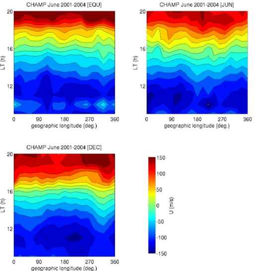
ionospheric dynamics is the zonal wind. Figure 2 shows the observed mean zonal wind above the magnetic equator at about 400 km altitude. Colour-coded velocities are plotted into GLON versus LT frames separately for each of the three seasons. The standard deviation and standard error of the mean are calculated in each bin (GLON×LT×season). Be-tween 09:00 LT and 20:00 LT the standard deviation (stan-dard error of the mean) in each bin is 40–50 m s−1 (4– 5 m s−1) on average. These values are smaller than the natu-ral diurnal variation range of zonal wind velocity (i.e. within about ±150 m s−1). This means that Fig. 2 closely repre-sents the diurnal behaviour of zonal wind. CHAMP obser-vations reveal the well-known characteristics of the low-latitude zonal wind: westward (negative) winds prevail dur-ing daytime and eastward in the evendur-ing (e.g. Coley et al., 1994). The direction switches around 16:00 LT. On a diurnal cycle the westward wind maximizes before noon. The day-time westward wind speed is higher than 100 m s−1_around

the diurnal peak.

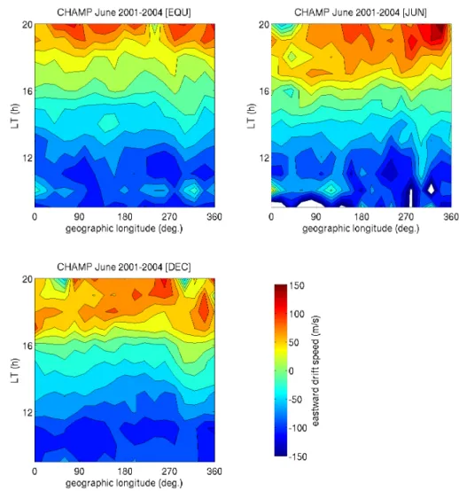
The zonal plasma drift (vy) as estimated from Eq. (3) is

(4)

Fig. 2.Average cross-track (nearly zonal) wind velocity estimated from the CHAMP observations. Each panel corresponds to a season.

shown in Fig. 2. Equation (3) contains an empirical relation of the Pedersen conductivity, whose accuracy is not known to us, and we have introduced several assumptions to solve Eq. (3). Hence, it is not straightforward to determine error bars forvyin Fig. 3. Instead we describe the sensitivity of vyin Fig. 3 to some independent variables. First, the spread

of zonal wind speed, as shown in the preceding paragraph, enters directly the spread ofvy(see Eq. 3). Second, thevy

in Fig. 3 is affected by the assumed value ofTr. We have

usedTr=1000 K and 1400 K. Both of the values lead to

de-viations, with respect to the case ofTr=1200 K, at most by

18 m s−1. As the variation range ofvyis about±100 m s−1,

these uncertainties cannot compromise the results presented in Fig. 3 severely.

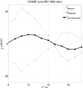
From Eq. (1) we know that both the zonal wind and the vertical component of the polarization electric field (or, equivalently, the zonal plasma drift) contribute to the F re-gion vertical current. The net current density can be es-timated from CHAMP magnetic field measurements using Eq. (2) (see also L¨uhr and Maus, 2006). Combining CHAMP

observations (FGM, PLP, and ACC) we can also quantify the relative contributions of the two constituents to the net F region vertical current. Figure 4 shows a comparison of the current contributions averaged over all GLON sectors and seasons. As the right-hand side of Eq. (2) is obtained by the Fourier decomposition and linear regression, it is not straightforward to add error bars to Jnet in Fig. 4. Instead

we estimate the variability ofJnet as follows. The standard

error of the mean by within ±6◦ MLAT is 0.5–0.6 nT on

average, and the linear regression is conducted within the MLAT range. Therefore, the error of ∂b_∂xy is approximately (0.6 nT)/(6◦), which corresponds to an error of 0.7 nA m−2 forJnet. As described above, the standard error of the mean

zonal wind is generally 4–5 m s−1. This value corresponds to error of about 2 nA m−2forJdynamo. In general, these

er-rors are small in comparison to the variation ranges ofJnet, JPedersen, andJdynamo, implying that Fig. 4 shows

(5)

Fig. 3.Zonal plasma drift velocity estimated from CHAMP observations, in the same format as that of Fig. 2.

observed net current is therefore only a small fraction of the magnitude of the currents driven by the F region wind dy-namo. Still, the dominance of the F region wind dynamo controls the polarity of the net F region vertical currents. It is interesting to see that the independently measured wind ve-locity and current density switch their signs at nearby points around 16:00 LT.

To validate the zonal plasma drift (vy) in Fig. 3 we

consid-ered plasma drift data from ROCSAT-1. These measurements have been binned in the same way as the CHAMP readings. The ROCSAT-1 zonal plasma drifts, which were averaged within±1.5◦MLAT, are displayed in Fig. 5, in just the same format and colour scale as in Fig. 3. The standard devia-tion and standard error of the mean are calculated in each bin (GLON×LT×season). Between 09:00 LT and 20:00 LT the standard deviation (standard error of the mean) in each bin is 40–50 m s−1(about 1 m s−1) on average. These values are smaller than the variation range ofvy(i.e. within about

±100 m s−1), which suggests that Fig. 5 closely describes the representative behaviour ofvy. As a cross check we compare

our Fig. 5 with Su et al. (2009), who also used the ROCSAT-1 zonal drift data during a similar period of time. Notable fea-tures in Figs. 3–4 of Su et al. (2009) can be summarized as follows. In December–January daytimevygenerally exhibits

weaker LT dependence than in June–July. The magnitude of daytimevy in December–January is generally smaller than

that in June–July. Westward-to-eastward reversal time is gen-erally later (near 18:00 LT) in June–July than in December– January (near 16:00 LT). Westward-to-eastward reversal time in June–July (December–January) is latest (earliest) around 330◦E GLON. All these features are in good agreement with our Fig. 5.

In the following we compare Figs. 3 and 5 in detail. In both figures, vy reversal time during December solstice is

earlier around 330◦E GLON than in the other GLON sec-tors. For June solstice, drift reversal is latest around 330◦E GLON in Fig. 5 (ROCSAT-1), while this tendency is barely observable in Fig. 3 (CHAMP). Also, the diurnal variation range ofvy is slightly smaller for ROCSAT-1 (Fig. 5) than

(6)

Fig. 4.Comparison of the contributors to the net F region vertical current: the F region dynamo current driven by F region zonal wind and the F region Pedersen current driven by the polarization electric field.

ROCSAT-1 than for CHAMP around June solstice (by about 2 h in LT). Moreover, the peak westward drift as observed by ROCSAT-1 occurs in the afternoon sector, especially during equinoxes and June solstice. Note that the westward drift as estimated from CHAMP data (Fig. 3) generally maximizes before noon.

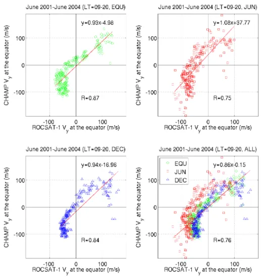
Figure 6 presents the correlation between vy from

ROCSAT-1 (x-axis) and CHAMP (y-axis) separately for each season in the form of scatter plots. The bottom-right panel contains all the data points combined. Each point in Fig. 6 corresponds to one bin in Figs. 3 and 5 (GLON×LT×season). The correlation coefficients are quite high. For December and equinox seasons they reach almost 0.9, which confirms the close agreement between the two independent data sets. Also the slopes of the ro-bust linear regression lines are close to unity (see the equa-tions in each panel). Of the three seasons, the correla-tion coefficient is lowest during June solstice, but still as high as 0.75. Some systematic differences between CHAMP and ROCSAT-1 are worth discussing. For highly negative (westward) velocities, ROCSAT-1 values go into saturation with respect to those estimated by CHAMP. Conversely, ROCSAT-1 observes slightly larger positive (eastward) ve-locities than those estimated by CHAMP except for June solstice. Good agreements are achieved in the rangevy=

±50 m s−1. During June solstice months a bias between the ROCSAT-1 data and CHAMP estimates appears to be about

−50 m s−1_{, which leads to the large intercept (37.8 m s}₋1_{) of}

the regression equation. In summary, the zonal plasma drifts from ROCSAT-1 and CHAMP are in qualitative agreement, but there are non-negligible offsets and differences between them, especially near the westward velocity peak and drift reversal.

4 Discussion

In this study we have presented the distribution of zonal plasma drift at low latitudes, estimated indirectly from CHAMP observations. The method was suggested earlier by Park and L¨uhr (2012), but applied then only to a limited pe-riod around the major sudden stratospheric warming (SSW) event in December 2001. For a qualitative verification, Park and L¨uhr (2012) compared their results (averaged over all the GLON sectors) with the climatological drift model of Fejer et al. (2005) (obtained at Jicamarca).

In the current study we make use of CHAMP and ROCSAT-1 measurements during 3 years of high solar activ-ity. This larger data set results in a finer resolution in GLON, LT, and season. CHAMP estimates have been directly com-pared with ROCSAT-1 plasma drift observations for valida-tion purposes. Since the orbits of the two satellites are very different in terms of altitudes and inclination angles, a statis-tical approach is used: the twovyvalues are compared in bins

of GLON, LT, and season. A favourable correlation coeffi-cient,R_≥0.84 during December solstice and equinox, con-firms the general agreement of plasma drift velocities from the two satellites. Also, the ratio between the two drift veloc-ities is close to unity. We may conclude that thevyestimated

from CHAMP data has a reasonable reliability.

Concerning certain differences between ROCSAT-1 and CHAMP plasma drifts, we compare both results with pre-vious works. Fejer et al. (2005) conducted a climatological study on zonal plasma drift above Jicamarca near the F re-gion peak (typically 300–500 km), which is similar to the CHAMP orbit altitude. For high solar activity periods, day-time westward drift in general maximizes at 11:30–12:00 LT, 12:30–13:00 LT, and 11:00–11:30 LT during equinox, June solstice, and December solstice, respectively (Fejer et al., 2005, Fig. 1). In our Fig. 3 westward drifts estimated by CHAMP around 280◦_{E GLON generally peak at 09:00–} 11:00 LT during the three respective seasons. In the same GLON sector, our Fig. 5 shows westward drift maxima for ROCSAT-1 generally at 12:00–13:00 LT during the three re-spective seasons. Concerning the LT of maximum westward drift, the results of Fejer et al. (2005) show better agreement with ROCSAT-1 data (our Fig. 5) than with CHAMP esti-mates (our Fig. 3).

(7)

Fig. 5.Same as Fig. 2, but for average zonal plasma drift velocity observed by the ROCSAT-1/IPEI.

280◦E GLON generally reverses from westward to east-ward at 15:00–16:00 LT. Compared to Fejer et al. (2005) the reversals in CHAMP data appear about an hour early. In the case of ROCSAT-1 (see our Fig. 5) the reversal times at 280◦E GLON are 16:00–17:00 LT, 17:00–18:00 LT, and 15:00–16:00 LT during the respective seasons. According to Su et al. (2009) mean reversal times in the Jicamarca sector are 16:40 LT and 15:20 LT for June and December solstice months, respectively, which is consistent with our Fig. 5. Concerning the LT ofvyreversal, ROCSAT-1 measurements

are in better agreement with Fejer et al. (2005) than CHAMP estimates are.

According to the San Marco D observations at 350– 700 km apex altitudes (Maynard et al., 1995, Fig. 4), vy

changes sign near 16:00 LT in equinox and solstice. Note that these observations are not limited to the Jicamarca lo-cation. In our Figs. 3 and 4, the reversal times of CHAMPvy

are slightly before 16:00 LT on average. In our Fig. 5 and Fig. 4 of Su et al. (2009) the reversal times of ROCSAT-1 vy are near 17:00 LT on average. Hence, the vy reversal

time of San Marco-D data (16:00 LT) is consistent with the CHAMP estimates rather than with the ROCSAT-1 observa-tions.vyreversal time in Fig. 3 (CHAMP) depends little on

seasons. Conversely, ROCSAT-1 measurements in our Fig. 5 and in Su et al. (2009, Fig. 4) show that thevyreversal time is

much later during June solstice than in the other seasons. As a consequence, the intercept of the regression line in Fig. 6 is largest during June solstice (about 40 m s−1_{), which}

corre-sponds to the delayed reversal of ROCSAT-1vywith respect

to CHAMPvy. We note that the reversal time in Maynard et

al. (1995, Fig. 4) and Fejer et al. (2005, Fig. 2) exhibits no conspicuous delay during June solstice, which agrees with our Fig. 3 (CHAMP) rather than with our Fig. 5 (ROCSAT-1). Daytime westward drift shown in Maynard et al. (1995, Fig. 4) maximizes at 13:00 LT for both equinox and solstice. It is in better agreement with ROCSAT-1 observations (our Fig. 5) than with CHAMP estimates (our Fig. 3).

As discussed in the preceding paragraphs,vymeasured by

(8)

Fig. 6.The correlation diagram between Figs. 3 and 5 for each season. The bottom-right panel contains all the data points in the other panels.

westward drift. Concerning these differences, previous stud-ies generally support the ROCSAT-1 observations, but not always (e.g. Maynard et al., 1995, Fig. 4). Hence, there seem to be multiple factors that compromise the agreement ofvy between CHAMP and ROCSAT-1. First, assumptions

used forvyestimation from CHAMP data can contribute to

the discrepancies. Especially, the empirical equation of ion-neutral collision frequency (νin=3.67×10−17nn√Tr(1−

0.064 log10Tr)2) may need additional correction terms

de-pending on LT, GLON, and season. Second, CHAMP obser-vations may also have some uncertainties, e.g. zonal wind un-certainty of about 20 m s−1as mentioned by Liu et al. (2006). Also,vy measured by ROCSAT-1 may have non-negligible

uncertainties as the velocity component is deduced primar-ily from the along-track drift measurements. For this com-ponent an uncertainty of±37.8∼75.45 m s−1 is quoted in http://cdaweb.gsfc.nasa.gov/misc/NotesR.html.

We discuss the relative contributions from the ionospheric E and F regions to the vertical currents in the equatorial F region. The daytimevyat F region altitudes is driven

primar-ily by the meridional electric field generated in the E layer

(e.g. Heelis, 2004, Eq. 11). This electric field maps up from low latitudes to CHAMP and ROCSAT-1 altitudes and causes the zonal plasma flow. The zonal wind in the F region blows in the same direction as the plasma drift (westward during daytime and eastward in the evening and at night), thus ex-periencing a much reduced ion drag. In our Figs. 2–3 the neutral wind is generally faster (in magnitude) than the ion drift, which agrees with Coley et al. (1994, Fig. 2). In our Fig. 4 we show the large and oppositely directed contribu-tion of the zonal neutral wind andvy(vertical polarization E

field) to F region vertical currents, which has not been appre-ciated appropriately in some of the earlier studies (e.g. L¨uhr and Maus, 2006; Park et al., 2010). Our observations demon-strate not only that the E region is a high-conductivity load for the F region wind dynamo currents, but also that the E field generated by E region zonal wind affects the net F re-gion vertical current significantly via the polarization electric field.

(9)

the F region are available. The reliability of the estimation will be improved when we have further information on ion temperature and composition (see Eq. 3), which were un-available for this study. The upcoming constellation mission of the European Space Agency, “Swarm”, consists of three identical CHAMP-like satellites. The Swarm satellites can measure all the ionospheric parameters obtained by CHAMP as well as ion temperature, composition, and drift velocity. The ion temperature and composition can give further con-straints to Eq. (3), and the estimated vy can be compared

directly to vy measured by Swarm. Moreover, one of the

Swarm satellites will be at higher altitudes than the oth-ers. This formation may help to clarify whether some of the discrepancies between the CHAMP estimation and the ROCSAT-1 observation (see Fig. 6) reflect a real altitude de-pendence ofvy. With the advent of the next solar maximum,

when the F region vertical currents are expected to be strong and clearly measurable, the Swarm satellites should provide an opportunity to validate our method ofvyestimation more

thoroughly and extensively.

5 Summary

Following the method suggested by Park and L¨uhr (2012), we have estimated zonal plasma drift velocity in the 09:00– 20:00 LT sector using electron/neutral/magnetic observations of CHAMP. For the period from June 2001 to June 2004 the estimated values are validated against ion drift measurements by ROCSAT-1/IPEI, and are compared with results from pre-vious ionospheric studies. Our main conclusions can be sum-marized as follows:

1. The plasma drifts estimated from CHAMP data are in reasonable agreement with the measurements by ROCSAT-1. A direct comparison of the data reveals a high linear correlation (R_≈0.8) for data obtained be-tween 09:00 and 20:00 LT. The slope of the regression line is close to unity for all seasons (Fig. 6).

2. vyestimated from CHAMP data show some

discrepan-cies with the ROCSAT-1 measurements.vy measured

by ROCSAT-1 (estimated from CHAMP data) gener-ally exhibits peak westward velocities after (before) noon. The reversal from westward to eastward zonal plasma drift, as estimated from CHAMP data, is earlier by about 1–2 h than ROCSAT-1 observations. Concern-ing these differences, some previous studies support the ROCSAT-1 observations, while others agree better with the CHAMP estimates.

3. During most parts of daytime, zonal wind and plasma drift generally point in the same direction in the equa-torial F region. This significantly reduces the ion drag effect on the neutrals. The reduced ion drag is one of the main causes of the high wind speeds along the mag-netic equator, as reported by Liu et al. (2009).

4. Zonal wind and plasma drift (or, equivalently, vertical polarization E field) contribute to the vertical F region current in opposite directions: e.g. an eastward wind drives upward currents, while an eastward plasma drift (or, equivalently, downward polarization E-field) causes downward current. In general the former effect (u_×B

wind dynamo) is lager in magnitude than the latter (Ped-ersen current), determining the direction of the net ver-tical current in the equatorial F region.

Acknowledgements. The CHAMP mission was sponsored by the Space Agency of the German Aerospace Center (DLR) through funds of the Federal Ministry of Economics and Technology, fol-lowing a decision of the German Federal Parliament (grant code 50EE0944). The CDAWeb data were obtained from the interface at http://cdaweb.gsfc.nasa.gov/. We are also grateful to the NCU ROCSAT-1/IPEI team members for their efforts in processing the ROCSAT-1/IPEI data.

The service charges for this open access publication have been covered by a Research Centre of the Helmholtz Association.

Topical Editor K. Hosokawa thanks two anonymous referees for their help in evaluating this paper.

References

Basu, S., MacKenzie, E., and Basu, S.: Ionospheric con-straints on VHF/UHF communications links during solar maximum and minimum periods, Radio Sci., 23, 363–378, doi:10.1029/RS023i003p00363, 1988.

Basu, S., Basu, S., Groves, K. M., Yeh, H.-C., Su, S.-Y., Rich, F. J., Sultan, P. J., and Keskinen, M. J.: Response of the equatorial ionosphere in the South Atlantic Region to the Great Magnetic Storm of July 15, 2000, Geophys. Res. Lett., 28, 3577–3580, doi:10.1029/2001GL013259, 2001.

Chen, G., Zhao, Z., Ning, B., Deng, Z., Yang, G., Zhou, C., Yao, M., Li, S., and Li, N.: Latitudinal dependence of the ionospheric response to solar eclipse of 15 January 2010, Geophys. Res. Lett., 116, A06301, doi:10.1029/2010JA016305, 2011.

Coley, W. R., Heelis, R. A., and Spencer, N. W.: Comparison of low-latitude ion and neutral zonal drifts using DE 2 data, J. Geophys. Res., 99, 341–348, doi:10.1029/93JA02205, 1994.

de Paula, E. R., Kantor, I. J., Sobral, J. H. A., Takahashi, H., San-tana, D. C., Gobbi, D., de Medeiros, A. F., Limiro, L. A. T., Kil, H., Kintner, P. M., and Taylor, M. J.: Ionospheric irregu-larity zonal velocities over Cachoeira Paulista, J. Atmos. Solar Terr. Phys., 64, 1511–1516, ISSN 1364-6826, 10.1016/S1364-6826(02)00088-3, 2002.

England, S. L. and Immel, T. J.: An empirical model of the drift velocity of equatorial plasma depletions, J. Geophys. Res., 117, A12308, doi:10.1029/2012JA018091, 2012.

(10)

ROCSAT-1 observations, J. Geophys. Res., 113, A05304, doi:10.1029/2007JA012801, 2008.

Hartman, W. A. and Heelis, R. A.: Longitudinal variations in the equatorial vertical drift in the topside ionosphere, J. Geophys. Res., 112, A03305, doi:10.1029/2006JA011773, 2007.

Heelis, R. A.: Electrodynamics in the low and middle latitude iono-sphere: a tutorial, J. Atmos. Solar Terr. Phys., 66, 825–838, doi:10.1016/j.jastp.2004.01.034, 2004.

Jee, G., Schunk, R. W., and Scherliess, L.: Analysis of TEC data from the TOPEX/Poseidon mission, J. Geophys. Res., 109, A01301, doi:10.1029/2003JA010058, 2004.

Kil, H., Kintner, P. M., de Paula, E. R., and Kantor, I. J.: Latitudinal variations of scintillation activity and zonal plasma drifts in South America, Radio Sci., 37, 1006, doi:10.1029/2001RS002468, 2002.

Kil, H., Oh, S.-J., Kelley, M. C., Paxton, L. J., England, S. L., Talaat, E., Min, K.-W., and Su, S.-Y.: Longitudinal structure of the verti-cal E×B drift and ion density seen from ROCSAT-1, Geophys. Res. Lett., 34, L14110, doi:10.1029/2007GL030018, 2007. Liu, H., L¨uhr, H., Watanabe, S., K¨ohler, W., Henize, V., and

Visser, P.: Zonal winds in the equatorial upper thermo-sphere: Decomposing the solar flux, geomagnetic activity, and seasonal dependencies, J. Geophys. Res., 111, A07307, doi:10.1029/2005JA011415, 2006.

Liu, H., Watanabe, S., and Kondo, T.: Fast thermospheric wind jet at the Earth’s dip equator, Geophys. Res. Lett., 36, L08103, doi:10.1029/2009GL037377, 2009.

L¨uhr, H. and Maus, S.: Direct observation of the F region dynamo currents and the spatial structure of the EEJ by CHAMP, Geo-phys. Res. Lett., 33, L24102, doi:10.1029/2006GL028374, 2006. Manju, G., Sreeja, V., Ravindran, S., and Thampi, S. V.: To-ward prediction of L band scintillations in the equatorial ionization anomaly region, J. Geophys. Res., 116, A02307, doi:10.1029/2010JA015893, 2011.

Martinis, C., Eccles, J. V., Baumgardner, J., Manzano, J., and Mendillo, M.: Latitude dependence of zonal plasma drifts ob-tained from dual-site airglow observations, J. Geophys. Res., 108, 1129, doi:10.1029/2002JA009462, 2003.

Maynard, N. C., Aggson, T. L., Herrero, F. A., Liebrecht, M. C., and Saba, J. L.: Average equatorial zonal and vertical ion drifts de-termined from San Marco D electric field measurements, J. Geo-phys. Res., 100, 17465–17479, doi:10.1029/95JA00767, 1995.

Nishioka, M., Basu, Su., Basu, S., Valladares, C. E., Sheehan, R. E., Roddy, P. A., and Groves, K. M.: C/NOFS satellite observations of equatorial ionospheric plasma structures supported by multi-ple ground-based diagnostics in October 2008, J. Geophys. Res., 116, A10323, doi:10.1029/2011JA016446, 2011.

Noja, M., Stolle, C., Park, J., and L¨uhr, H.: Long term analysis of ionospheric polar patches based on CHAMP TEC data, Radio Sci., in press, doi:10.1002/rds.20033, 2013.

Pacheco, E. E., Heelis, R. A., and Su, S.-Y.: Superrotation of the ionosphere and quiet time zonal ion drifts at low and middle lati-tudes observed by Republic of China Satellite-1 (ROCSAT-1), J. Geophys. Res., 116, A11329, doi:10.1029/2011JA016786, 2011. Park, J. and L¨uhr, H.: Effects of sudden stratospheric warming (SSW) on the lunitidal modulation of the F region dynamo, J. Geophys. Res., 117, A09320, doi:10.1029/2012JA018035, 2012. Park, J., L¨uhr, H., and Min, K. W.: Characteristics of F region dynamo currents deduced from CHAMP mag-netic field measurements, J. Geophys. Res., 115, A10302, doi:10.1029/2010JA015604, 2010.

Sastri, J. H.: Longitudinal dependence of equatorial F region verti-cal plasma drifts in the dusk sector, J. Geophys. Res., 101, 2445– 2452, doi:10.1029/95JA02759, 1996.

Scherliess, L. and Fejer, B. G.: Radar and satellite global equatorial F region vertical drift model, J. Geophys. Res., 104, 6829–6842, doi:10.1029/1999JA900025, 1999.

Schunk, R. W. and Nagy, A. F.: Ionospheres: Physics, Plasma Physics, and Chemistry, Second Edition, Cambridge Univ. Press, 2009.

Stolle, C., Manoj, C., L¨uhr, H., Maus, S., and Alken, P.: Es-timating the daytime Equatorial Ionization Anomaly strength from electric field proxies, J. Geophys. Res., 113, A09310, doi:10.1029/2007JA012781, 2008.

Su, S.-Y., Yeh, H. C., and Heelis, R. A.: ROCSAT 1 ionospheric plasma and electrodynamics instrument observations of equato-rial spread F: An early transitional scale result, J. Geophys. Res., 106, 29153–29159, doi:10.1029/2001JA900109, 2001.