www.atmos-meas-tech.net/9/2497/2016/ doi:10.5194/amt-9-2497-2016
© Author(s) 2016. CC Attribution 3.0 License.
Ground-based assessment of the bias and long-term stability of
14 limb and occultation ozone profile data records
Daan Hubert1, Jean-Christopher Lambert1, Tijl Verhoelst1, José Granville1, Arno Keppens1, Jean-Luc Baray2,3, Adam E. Bourassa4, Ugo Cortesi5, Doug A. Degenstein4, Lucien Froidevaux6, Sophie Godin-Beekmann7,
Karl W. Hoppel8, Bryan J. Johnson9, Erkki Kyrölä10, Thierry Leblanc11, Günter Lichtenberg12, Marion Marchand7, C. Thomas McElroy13, Donal Murtagh14, Hideaki Nakane15,16, Thierry Portafaix2, Richard Querel17,
James M. Russell III18, Jacobo Salvador19, Herman G. J. Smit20, Kerstin Stebel21, Wolfgang Steinbrecht22, Kevin B. Strawbridge23, René Stübi24, Daan P. J. Swart25, Ghassan Taha26,27, David W. Tarasick23,
Anne M. Thompson27, Joachim Urban14,†, Joanna A. E. van Gijsel28, Roeland Van Malderen29, Peter von der Gathen30, Kaley A. Walker31,32, Elian Wolfram19, and Joseph M. Zawodny33 1Royal Belgian Institute for Space Aeronomy (BIRA-IASB), Brussels, Belgium
2Laboratoire de l’Atmosphère et des Cyclones (Université de La Réunion, CNRS, Météo-France), OSU-Réunion (Université de La Réunion, CNRS), La Réunion, France
3Laboratoire de Météorologie Physique, Observatoire de Physique du Globe de Clermont-Ferrand (Université Blaise Pascal, CNRS), Clermont-Ferrand, France
4Institute of Space and Atmospheric Studies, University of Saskatchewan, Saskatoon, SK, Canada
5Istituto di Fisica Applicata “Nello Carrara” del Consiglio Nazionale delle Ricerche, Sesto Fiorentino, Italy 6Jet Propulsion Laboratory, California Institute of Technology, Pasadena, CA, USA
7Laboratoire Atmosphère Milieux Observations Spatiales, Université de Versailles Saint-Quentin en Yvelines, Centre National de la Recherche Scientifique, Paris, France
8Naval Research Lab, Washington, DC, USA
9NOAA Earth System Research Laboratory, Global Monitoring Division, Boulder, Colorado, USA 10Finnish Meteorological Institute, Helsinki, Finland
11Jet Propulsion Laboratory, California Institute of Technology, Wrightwood, CA, USA
12German Aerospace Center (DLR), Remote Sensing Technology Institute, Oberpfaffenhofen, Germany 13York University, Toronto, ON, Canada
14Department of Earth and Space Sciences, Chalmers University of Technology, Göteborg, Sweden 15Kochi University of Technology, Kochi, Japan
16National Institute for Environmental Studies, Tsukuba, Ibaraki, Japan 17National Institute of Water and Atmospheric Research, Lauder, New Zealand 18Department of Atmospheric and Planetary Science, Hampton University, VA, USA
19CEILAP-UNIDEF (MINDEF-CONICET), UMI-IFAECI-CNRS-3351, Villa Martelli, Argentina
20Research Centre Jülich, Institute for Energy and Climate Research: Troposphere (IEK-8), Jülich, Germany 21Norwegian Institute for Air Research (NILU), Kjeller, Norway
22Meteorologisches Observatorium, Deutscher Wetterdienst, Hohenpeissenberg, Germany 23Air Quality Research, Environment and Climate Change Canada, Toronto, ON, Canada 24Payerne Aerological Station, MeteoSwiss, Payerne, Switzerland
25National Institute for Public Health and the Environment (RIVM), Bilthoven, the Netherlands 26Universities Space Research Association, Greenbelt, MD, USA
27NASA Goddard Space Flight Center, Greenbelt, MD, USA
28Royal Netherlands Meteorological Institute (KNMI), De Bilt, the Netherlands 29Royal Meteorological Institute of Belgium, Brussels, Belgium
31Department of Physics, University of Toronto, Toronto, ON, Canada 32Department of Chemistry, University of Waterloo, Waterloo, ON, Canada 33NASA Langley Research Center, Hampton, VA, USA
†deceased
Correspondence to:D. Hubert ([email protected])
Received: 19 March 2015 – Published in Atmos. Meas. Tech. Discuss.: 2 July 2015 Revised: 28 April 2016 – Accepted: 14 May 2016 – Published: 8 June 2016
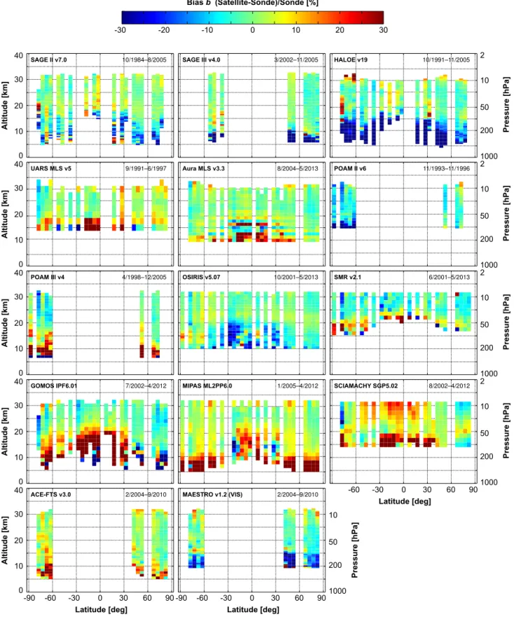
Abstract. The ozone profile records of a large number of limb and occultation satellite instruments are widely used to address several key questions in ozone research. Further progress in some domains depends on a more detailed un-derstanding of these data sets, especially of their long-term stability and their mutual consistency. To this end, we made a systematic assessment of 14 limb and occultation sounders that, together, provide more than three decades of global ozone profile measurements. In particular, we considered the latest operational Level-2 records by SAGE II, SAGE III, HALOE, UARS MLS, Aura MLS, POAM II, POAM III, OSIRIS, SMR, GOMOS, MIPAS, SCIAMACHY, ACE-FTS and MAESTRO. Central to our work is a consistent and ro-bust analysis of the comparisons against the ground-based ozonesonde and stratospheric ozone lidar networks. It al-lowed us to investigate, from the troposphere up to the stratopause, the following main aspects of satellite data qual-ity: long-term stability, overall bias and short-term variabil-ity, together with their dependence on geophysical parame-ters and profile representation. In addition, it permitted us to quantify the overall consistency between the ozone profilers. Generally, we found that between 20 and 40 km the satel-lite ozone measurement biases are smaller than ±5 %, the
short-term variabilities are less than 5–12 % and the drifts are at most ±5 % decade−1 (or even±3 % decade−1 for a few
records). The agreement with ground-based data degrades somewhat towards the stratopause and especially towards the tropopause where natural variability and low ozone abun-dances impede a more precise analysis. In part of the strato-sphere a few records deviate from the preceding general con-clusions; we identified biases of 10 % and more (POAM II and SCIAMACHY), markedly higher single-profile vari-ability (SMR and SCIAMACHY) and significant long-term drifts (SCIAMACHY, OSIRIS, HALOE and possibly GO-MOS and SMR as well). Furthermore, we reflected on the repercussions of our findings for the construction, analy-sis and interpretation of merged data records. Most notably, the discrepancies between several recent ozone profile trend assessments can be mostly explained by instrumental drift. This clearly demonstrates the need for systematic compre-hensive multi-instrument comparison analyses.
1 Introduction
Long-term global observations of the distribution and evolu-tion of ozone are vital to improve our current understanding of atmospheric processes, and thereby to allow more robust projections of the recovery of the ozone layer and climate change. Measurements of the vertical profile of ozone have been carried out over the last few decades by a large num-ber of instruments, operating in situ or from remote vantage points, on the ground and in space (for an overview, see Has-sler et al., 2014). These indisputably show globally declining ozone levels during the 1980s and a large part of the 1990s in the lower and upper stratosphere (∼5–7 % decade−1),
and to a lesser extent also in the middle stratosphere (1– 2 % decade−1) (WMO, 2014; Harris et al., 2015). Further-more, the observed loss rates are in excellent agreement with expectations for the chemical destruction of ozone by man-made halocarbons (WMO, 2014). The abundances of these substances have decreased significantly over the past 15– 20 years (WMO, 2011), as a result of the Montreal Protocol and its subsequent adjustments and amendments. It is thefore generally expected that the ozone layer is currently re-covering from the effects of ozone depleting substances, al-beit in an atmosphere with concomitant increases in green-house gas concentrations and changes in residual circula-tion (Waugh et al., 2009; Oman et al., 2010). While obser-vations provide substantial evidence for the levelling off of the downward trend around 1997 at most latitudes and alti-tudes, i.e. the first phase of recovery, it is less clear whether they support an upward trend in recent years (Harris et al., 2015). Whether the onset of the second stage has been de-tected (or not) is one of the key questions in current ozone research, a debate that is hampered by two factors. The first is the small magnitude of the increases in ozone (a few per-cent) when compared to its natural variability. This can only be remedied by longer time series. And the second is the lack of appropriate knowledge of the uncertainties in the observa-tional records. Shedding more light on the latter issue is the main objective of this paper.
than a decade, so their records are generally combined for long-term studies. The uncertainties (overall bias, short-term variability and long-term stability) in the resulting combined data set are an intricate combination of the uncertainties in-herited from the contributing data sets and those introduced by the merging algorithm. Tummon et al. (2015) recently noted that the former source of error tends to dominate over the latter, thereby demonstrating the need for a detailed char-acterization of each individual record and especially of their mutual consistency.
Numerous validation studies have been published in recent years (for an overview, see Hubert et al., 2016), but some important gaps remain. First of all, there are no comprehen-sive multi-instrument assessments of most limb/occultation sounders using ground-based data as a reference. Also satel-lite intercomparison studies rarely cover more than a hand-ful of records (exceptions are, e.g. Dupuy et al., 2009; Jones et al., 2009; Laeng et al., 2014; Rahpoe et al., 2015). Tegt-meier et al. (2013) conducted perhaps the most complete as-sessment so far, of the ozone climatologies from 18 sounders. Like most works, it was dedicated to the quantification of bias patterns and shorter-term variability, but not to a detailed assessment of the stability on decadal time scales. However, precise estimates of instrumental drift are crucial for a sound determination of the significance of trend results. Just a few (in some cases indirect) drift estimates are available from ground-based comparisons (e.g. Terao and Logan, 2007; Nair et al., 2012) or from satellite intercomparisons (e.g. Jones et al., 2009; Mieruch et al., 2012; Adams et al., 2014; Eck-ert et al., 2014; Rahpoe et al., 2015). Moreover, no works comprise all the records considered in the recent trend as-sessments, by, e.g. the World Meteorological Organisation (WMO) (WMO, 2014) or within the SPARC/IO3C/IGACO-O3/NDACC (SI2N) initiative (for an overview, see Harris et al., 2015). Finally, the quality of auxiliary pressure and temperature profiles plays a role too, as it unavoidably affects the quality of ozone data when used to convert the ozone profiles to another vertical coordinate (altitude↔pressure) or ozone quantity (number density↔volume mixing ratio),
a common step in the merging process. At the moment, very little information on this latter aspect of data quality is avail-able.
Our objective is to shed more light on these three miss-ing pieces of information. We therefore perform an ex-haustive assessment, from the ground up to the stratopause, of the latest releases of the operational Level-2 ozone profile data sets collected by 14 limb/occultation instru-ments over the period 1984–2013: SAGE II (v7), SAGE III (v4), HALOE (v19), UARS MLS (v5), Aura MLS (v3.3), POAM II (v6), POAM III (v4), OSIRIS (v5.07), SMR (v2.1), GOMOS (IPF 6), MIPAS (ML2PP 6), SCIAMACHY (SGP 5), ACE-FTS (v3) and MAESTRO (v1.2). Each satel-lite data set is compared to the observations by the ground-based ozonesonde and stratospheric ozone lidar networks, thereby acting as a pseudo-global, independent and
well-characterised transfer standard. The robust analysis of co-located satellite-ground profile pairs allows us to quantify overall bias, short-term variability and long-term stability of the satellite records, and their dependence on altitude, lati-tude and season. Methodology and results for the native pro-file representation of each record are described in Sects. 3–5. In Sect. 6 we investigate whether the accompanying ancil-lary meteorological data impact ozone data quality when the original profiles are converted to another vertical coordinate or ozone quantity.
The adoption of a consistent analysis framework permits us to bring all single-instrument results together, and exam-ine the mutual consistency between instruments of each qual-ity indicator (Sect. 7). We report the tendencies and several peculiarities, most notably a few instruments that drift sig-nificantly at some altitudes. Finally, we frame our findings within the broader context (Sect. 8), by commenting on cur-rent challenges related to verifying user requirements, and by highlighting the implications of our results for the design of merging schemes. Perhaps the most tangible outcome of our study is the successful interpretation of discrepancies in recent trend studies in terms of instrumental drift. It demon-strates that our work can contribute to a better exploitation of the limb and occultation ozone profile data sets. This should, in the end, be beneficial not only for trend assessments and the related merging activities, but also for other applications, such as trend attribution studies or model evaluations.
2 Ozone profile data records
Our assessment covers the period between October 1984 and May 2013 and considers 14 satellite missions and two types of ground-based instruments. We first present the ozone pro-file data records that play a central role in our analyses: those gathered by ozonesonde and stratospheric lidar instruments. Then, we introduce the limb and occultation sounders that are the subject of this work. We limit ourselves to brief descrip-tions since all space- and ground-based ozone profile mea-surement techniques were reviewed exhaustively by Hassler et al. (2014). The technical details most relevant to our as-sessment are summarised in Tables 1–3.
2.1 Ground-based network observations 2.1.1 Ozonesondes
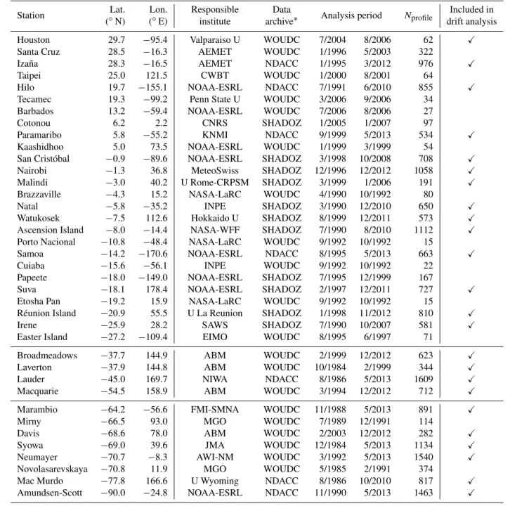
Table 1.Overview of the 72 ozonesonde stations considered in this work, their location and the archive the data were taken from. Time range and profile statistics reflect the total, screened sample straddling the analysis period (10/1984–5/2013), not the co-located sample (which differs per satellite instrument). All listed stations were used in the analyses of bias and comparison spread, those indicated in the last column were also used for the drift analysis.
Station Lat. Lon. Responsible Data Analysis period Nprofile Included in
(◦N) (◦E) institute archive∗ drift analysis
Alert 82.5 −62.5 EC WOUDC 12/1987 12/2011 1244 X
Eureka 80.0 −85.9 EC WOUDC 11/1992 9/2011 1318 X
Ny-Ålesund 78.9 11.9 AWI-NA WOUDC 10/1990 5/2013 2224 X
Thule 76.5 −68.7 DMI NDACC 10/1991 1/2013 349 X
Resolute 74.7 −95.0 EC WOUDC 10/1984 8/2011 1020 X
Summit 72.3 −38.3 NOAA-ESRL NDACC 2/2005 5/2013 427 X
Scoresbysund 70.5 −21.9 DMI NDACC 2/1989 5/2013 1169 X
Sodankylä 67.4 26.6 FMI NDACC 11/1991 12/2010 1085 X
Edmonton 53.5 −114.1 EC WOUDC 10/1984 8/2011 1193 X
Goose Bay 53.3 −60.4 EC WOUDC 10/1984 8/2011 1272 X
Lindenberg 52.2 14.1 DWD-MOL WOUDC 10/1984 5/2013 1660 X
De Bilt 52.1 5.2 KNMI NDACC 11/1992 12/2012 1061 X
Vanscoy 52.0 −107.0 EC WOUDC 8/1990 9/2004 60
Valentia 51.9 −10.2 ME WOUDC 1/1994 12/2012 555 X
Uccle 50.8 4.3 RMIB WOUDC 10/1984 6/2012 3712 X
Gimli 50.6 −97.0 EC WOUDC 7/1985 8/1985 10
Bratt’s Lake 50.2 −104.7 EC WOUDC 12/2003 9/2011 402 X
Praha 50.0 14.4 CHMI-PR WOUDC 1/1985 4/2013 1210 X
Kelowna 49.9 −119.4 EC WOUDC 11/2003 8/2011 432 X
Hohenpeißenberg 47.8 11.0 DWD-MOHp WOUDC 10/1984 5/2013 3586 X
Payerne 46.8 7.0 MeteoSwiss WOUDC 10/1984 12/2012 4052 X
Pellston 45.6 −84.7 NOAA-ESRL WOUDC 7/2004 8/2004 5
Pietro Capofiume 44.6 11.6 AM-IMS WOUDC 3/1991 12/1993 95
Egbert 44.2 −79.8 EC WOUDC 12/2003 8/2011 373 X
Yarmouth 43.9 −66.1 EC WOUDC 10/2003 8/2011 394 X
Sofia 42.8 23.4 BNIHM WOUDC 11/1984 12/1991 145
Trinidad Head 40.8 −124.2 NOAA-ESRL WOUDC 1/1999 8/2006 197 X
Madrid 40.5 −3.7 AEMET WOUDC 12/1994 5/2013 738 X
Boulder 40.0 −105.2 NOAA-ESRL NDACC 6/1991 5/2013 1097 X
Beltsville 39.0 −76.5 Howard U WOUDC 8/2006 8/2006 12
Huntsville 34.7 −86.6 UAH WOUDC 4/1999 12/2007 574 X
Table Mountain 34.4 −117.7 NASA-JPL WOUDC 2/2006 8/2006 35 X
Isfahan 32.5 51.4 MDI WOUDC 7/1995 4/2011 151 X
Palestine 31.8 −95.7 EC WOUDC 5/1985 6/1985 26
characterisation and post-flight processing (see, e.g. Tara-sick et al., 2016; Van Malderen et al., 2016). However, when standard operating procedures are followed, the three most commonly used sonde types1produce consistent results be-tween the tropopause and∼28 km, with biases smaller than ±5 % and precisions better than∼3 % (Smit and
ASOPOS-panel, 2014). At higher and lower altitudes the data quality
1Nowadays more than 80 % of the stations launch an
electro-chemical concentration cell (ECC) sonde (Komhyr, 1969). The Brewer–Mast sonde has mostly been used by the early sounding stations with long data records (Brewer and Milford, 1960), while the Japanese stations fly a carbon iodine cell sonde (Kobayashi and Toyama, 1966).
degrades somewhat, and the differences between the sonde types become more clear. Overall, ECC-type sondes per-form best with a bias of±5–7 % and a precision of 3–5 %
Table 1.Continued.
Station Lat. Lon. Responsible Data Analysis period Nprofile Included in
(◦N) (◦E) institute archive∗ drift analysis
Houston 29.7 −95.4 Valparaiso U WOUDC 7/2004 8/2006 62 X
Santa Cruz 28.5 −16.3 AEMET WOUDC 1/1996 5/2003 322
Izaña 28.3 −16.5 AEMET NDACC 1/1995 3/2012 976 X
Taipei 25.0 121.5 CWBT WOUDC 1/2000 8/2001 64
Hilo 19.7 −155.1 NOAA-ESRL NDACC 7/1991 6/2010 855 X
Tecamec 19.3 −99.2 Penn State U WOUDC 3/2006 9/2006 34
Barbados 13.2 −59.4 NOAA-ESRL WOUDC 7/2006 8/2006 27
Cotonou 6.2 2.2 CNRS SHADOZ 1/2005 1/2007 97
Paramaribo 5.8 −55.2 KNMI NDACC 9/1999 5/2013 534 X
Kaashidhoo 5.0 73.5 NOAA-ESRL WOUDC 1/1999 3/1999 54
San Cristóbal −0.9 −89.6 NOAA-ESRL SHADOZ 3/1998 10/2008 708 X
Nairobi −1.3 36.8 MeteoSwiss SHADOZ 12/1996 12/2012 1058 X
Malindi −3.0 40.2 U Rome-CRPSM SHADOZ 3/1999 1/2006 191 X
Brazzaville −4.3 15.2 NASA-LaRC WOUDC 4/1990 10/1992 80
Natal −5.8 −35.2 INPE SHADOZ 3/1990 12/2010 650 X
Watukosek −7.5 112.6 Hokkaido U SHADOZ 8/1999 12/2011 573 X
Ascension Island −8.0 −14.4 NASA-WFF SHADOZ 7/1990 8/2010 1112 X
Porto Nacional −10.8 −48.4 NASA-LaRC WOUDC 9/1992 10/1992 15
Samoa −14.2 −170.6 NOAA-ESRL NDACC 8/1995 5/2013 663 X
Cuiaba −15.6 −56.1 INPE WOUDC 9/1992 10/1992 22
Papeete −18.0 −149.0 NOAA-ESRL SHADOZ 7/1995 12/1999 167
Suva −18.1 178.4 NOAA-ESRL SHADOZ 2/1997 12/2011 727 X
Etosha Pan −19.2 15.9 NASA-LaRC WOUDC 9/1992 10/1992 15
Réunion Island −20.9 55.5 U La Reunion SHADOZ 1/1998 11/2012 810 X
Irene −25.9 28.2 SAWS SHADOZ 7/1990 10/2007 581 X
Easter Island −27.2 −109.4 EIMO WOUDC 8/1995 6/1997 71
Broadmeadows −37.7 144.9 ABM WOUDC 2/1999 12/2012 623 X
Laverton −37.9 144.8 ABM WOUDC 10/1984 2/1999 344 X
Lauder −45.0 169.7 NIWA NDACC 8/1986 5/2013 1609 X
Macquarie −54.5 158.9 ABM WOUDC 3/1994 12/2012 712 X
Marambio −64.2 −56.6 FMI-SMNA WOUDC 11/1988 5/2013 891 X
Mirny −66.5 93.0 MGO WOUDC 7/1989 12/1991 114
Davis −68.6 78.0 ABM WOUDC 2/2003 12/2012 282 X
Syowa −69.0 39.6 JMA WOUDC 12/1984 5/2013 1134 X
Neumayer −70.7 −8.3 AWI-NM WOUDC 3/1992 5/2013 1540 X
Novolasarevskaya −70.8 11.9 MGO WOUDC 5/1985 2/1991 374
Mac Murdo −77.8 166.6 U Wyoming NDACC 8/1986 10/2010 817 X
Amundsen-Scott −90.0 −24.8 NOAA-ESRL NDACC 11/1990 5/2013 1463 X
∗Sources: NDACC, http://www.ndacc.org; WOUDC, http://www.woudc.org; SHADOZ, http://croc.gsfc.nasa.gov/shadoz.
profiles over the analysis period. The screening procedure is outlined in Sect. 3.
2.1.2 Stratospheric ozone lidars
Differential absorption lidars are laser-based active remote sensing systems that operate mostly during clear-sky nights. Profiles of ozone number density vs. geometric altitude are retrieved between the tropopause and 45–50 km from backscattered signals at two wavelengths (Mégie et al., 1977). While instrument and retrieval set-up differs from
one site to another, the NDACC ozone lidar network can be considered as homogeneous within 2 % between 20 and 35 km. In this altitude range both bias and precision are esti-mated at∼2 % and worsen to 5–10 % at other altitudes due
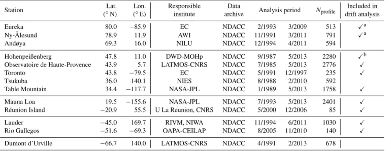
radiome-Table 2.Like Table 1, but for the 13 considered stratospheric ozone lidar stations.
Station Lat. Lon. Responsible Data Analysis period Nprofile Included in (◦N) (◦E) institute archive drift analysis
Eureka 80.0 −85.9 EC NDACC 2/1993 3/2009 513 Xa
Ny-Ålesund 78.9 11.9 AWI NDACC 11/1991 3/2011 791 Xa
Andøya 69.3 16.0 NILU NDACC 12/1994 4/2011 594
Hohenpeißenberg 47.8 11.0 DWD-MOHp NDACC 9/1987 5/2013 2280 Xb
Observatoire de Haute-Provence 43.9 5.7 LATMOS-CNRS NDACC 7/1985 5/2013 2776 X
Toronto 43.8 −79.5 EC NDACC 5/1991 12/1997 235 X
Tsukuba 36.0 140.1 NIES NDACC 8/1988 2/2010 592
Table Mountain 34.4 −117.7 NASA-JPL NDACC 1/1989 5/2013 1758 X
Mauna Loa 19.5 −155.6 NASA-JPL NDACC 7/1993 5/2013 2401 X
Réunion Island −20.9 55.5 U La Reunion, CNRS NDACC 5/2000 12/2006 85 X
Lauder −45.0 169.7 RIVM, NIWA NDACC 11/1994 6/2011 1030 X
Rio Gallegos −51.6 −69.3 OAPA-CEILAP NDACC 8/2005 11/2010 140 X
Dumont d’Urville −66.7 140.0 LATMOS-CNRS NDACC 4/1991 2/2013 678
aAll Arctic lidar data are discarded in the drift analysis of the SCIAMACHY record.
bHohenpeißenberg is only included in the drift analysis of satellite instruments that ceased operations prior to 2007.
ters (McGee et al., 1991; Keckhut et al., 2004). Furthermore, comparisons to space-based observations over the range 20– 40 km showed biases less than±5 % and a decadal stability
better than±5 % decade−1 (Nair et al., 2012). We use data
from 13 stratospheric ozone lidars in the NDACC network. Geographical location, measurement period and number of screened profiles over the analysis period are listed in Ta-ble 2. The screening procedure is outlined in Sect. 3. When-ever lidar data are converted to non-native profile representa-tions, we do so in this work using thep/T information ex-tracted at the time and location of the lidar measurement from the ERA-Interim reanalysis fields (Dee et al., 2011) produced by the European Centre for Medium-Range Weather Fore-casts (ECMWF).
2.2 Satellite observations
Over the past few decades numerous instruments were de-ployed in space to monitor atmospheric ozone. Detailed in-tercomparison studies of monthly zonal mean ozone profile data (i.e. Level-3) were published for nadir-viewing (Kra-marova et al., 2013) and limb/occultation-viewing instru-ments (Tegtmeier et al., 2013). Here, we focus on a ground-based validation of the Level-2 ozone profile records from 14 limb/occultation sounders that had (have) prime sensitivity in the stratosphere and were (are) operational for more than 3 years, see Table 3.
Most instruments were launched only once: HALOE (Halogen Occultation Experiment), OSIRIS (Optical Spec-trograph and InfraRed Imaging System), SMR (Sub-Millimetre Radiometer), GOMOS (Global Ozone Monitor-ing by Occultation of Stars), MIPAS (Michelson Interfer-ometer for Passive Atmospheric Sounding), SCIAMACHY
(SCanning Imaging Absorption spectroMeter for Atmo-spheric CHartographY), ACE-FTS (AtmoAtmo-spheric Chemistry Experiment Fourier Transform Spectrometer) and MAE-STRO (Measurements of Aerosol Extinction in the Strato-sphere and TropoStrato-sphere Retrieved by Occultation). Some were deployed more than once, with improved design: SAGE (Stratospheric Aerosol and Gas Experiment, II and III), MLS (Microwave Limb Sounder, on the UARS and EOS-Aura platforms) and POAM (Polar Ozone and Aerosol Measure-ment, II and III). Five instruments (OSIRIS, SMR, ACE-FTS, MAESTRO and Aura MLS) remain operational until the present, nine ceased operations before the end of the anal-ysis period (May 2013).
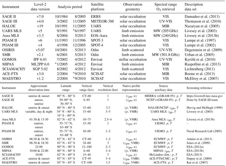
Table 3.Overview of satellite ozone profile data records. For more details on the instrument and the retrieval technique we refer to the review by Hassler et al. (2014). Some instrument teams recommend to discard a considerable part of their ozone record for long-term studies. The asterisk in the analysis period columns denotes whether the early or late part of the mission is cropped (see text).
Instrument Level-2 Analysis period Satellite Observation Spectral range Description data version platform geometry O3retrieval data set
SAGE II v7.0 10/1984 8/2005 ERBS solar occultation VIS Damadeo et al. (2013) SAGE III v4.0 3/2002 11/2005 METEOR-3M solar occultation UV-VIS Thomason et al. (2010) HALOE v19 10/1991 11/2005 UARS solar occultation MIR Nazaryan et al. (2005) UARS MLS v5 9/1991 ∗6/1997 UARS limb emission MW (205 GHz) Livesey et al. (2003) Aura MLS v3.3 8/2004 5/2013 EOS-Aura limb emission MW (240 GHz) Livesey et al. (2013b) POAM II v6 11/1993 11/1996 SPOT-3 solar occultation VIS Lumpe et al. (1997) POAM III v4 4/1998 12/2005 SPOT-4 solar occultation VIS Lumpe et al. (2002) OSIRIS v5.07 10/2001 5/2013 Odin limb scattered UV-VIS Degenstein et al. (2009) SMR v2.1 6/2001 5/2013 Odin limb emission MW (501.8 GHz) Urban et al. (2005) GOMOS IPF 6.01 7/2002 4/2012 Envisat stellar occultation UV-VIS Kyrölä et al. (2010) MIPAS ML2PP 6.0 ∗1/2005 4/2012 Envisat limb emission MIR Raspollini et al. (2013) SCIAMACHY SGP 5.02 8/2002 4/2012 Envisat limb scattered VIS Lichtenberg (2011) ACE-FTS v3.0 2/2004 ∗9/2010 SCISAT solar occultation MIR Boone et al. (2013) MAESTRO v1.2 2/2004 ∗9/2010 SCISAT solar occultation VIS McElroy et al. (2007)
Instrument observation timeApproximate Latituderange range (km)Vertical resolution (km)Vertical representationNative profile auxiliary dataSource Screening reference
SAGE II sunrise & sunset 80◦N – 80◦S CT–60 1 (z
gm,n) MERRA (+GRAM-95):p,T https://eosweb.larc.nasa.gov
SAGE III sunset, 50–80◦N, 6–85 1 (z
gm,n) NCEP (+GRAM-95):p,T Done by SAGE III team sunrise 30–50◦S
HALOE sunrise & sunset 80◦N – 80◦S 15–60 2.3 (p, VMR) HALOE/NCEP:zgm,T Hervig and McHugh (1999) UARS MLS variable, day & night 34◦N – 80◦S, 15–60 3–5 (p, VMR) UARS MLS:z
gp,T Livesey et al. (2003) 34◦S – 80◦N
Aura MLS 01:30 & 13:30 82◦N – 82◦S 10–75 2.5–4 (p, VMR) Aura MLS:z
gp,T Livesey et al. (2013b)
POAM II sunrise, 55–71◦N, 15–50 1 (z
gm,n) UKMO:p,T –
sunset 63–88◦S
POAM III sunrise, 55–71◦N, 10–60 1–2 (zgm,n) UKMO:p,T Naval Research Lab (2005) sunset 63–88◦S
OSIRIS 06:30 & 18:30 82◦N – 82◦S CT–60 1–2 (z
gm,n) ECMWF:p,T Adams et al. (2013) SMR 06:30 & 18:30 82◦N – 82◦S 18–60 3 (z
gm, VMR) ECMWF:p,T Jones et al. (2009)
GOMOS 22:00 90◦N – 90◦S 12–100 2–3 (z
gm,n) ECMWF:p,T ESA (2012a) MIPAS 10:00 & 22:00 80◦N – 80◦S 6–68 3–4 (p, VMR) MIPAS:zgm,T ESA (2012b)
SCIAMACHY 10:00 82◦N – 80◦S 15–40 3 (z
gm,n) McLinden clim.:p,T ESA (2013) ACE-FTS sunrise & sunset 85◦N – 85◦S CT–95 3–4 (z
gm, VMR) ACE-FTS/CMC:p/T Dupuy et al. (2009) MAESTRO sunrise & sunset 85◦N – 85◦S CT–100 1.5 (z
gm, VMR) ACE-FTS:p,T Kar et al. (2007) UV: ultraviolet; VIS: visible; MIR: mid-infrared; MW: microwave. CT stands for cloud top,pfor pressure,Tfor temperature,zgmfor geometric altitude,
zgpfor geopotential height, VMR for volume mixing ratio,nfor number density.
provides ozone data sets on both a variable and a fixed alti-tude grid, we pick the latter product.
A number of alternative data sets for these instruments were not included in this assessment. For instance the re-trievals by scientific prototype Level-2 processors (MIPAS, SCIAMACHY) were not considered here. Their bias struc-ture is often comparable to that of the operational ozone data set, especially when contrasted to that of other instru-ments (e.g. Rozanov et al., 2007; Laeng et al., 2015), due to the use of the same calibrated Level-1 radiance data and a common sensitivity to retrieval parameters (e.g. spectro-scopic data). Profile data from alternative viewing geome-tries (e.g. lunar occultations for SAGE III and SCIAMACHY, solar occultation data from SCIAMACHY or bright limb measurements by GOMOS) were not investigated either, and their quality may well be different from the findings pre-sented in the following.
Table 3 summarizes host platform, observation geometry and time, spectral region and spatial coverage. Vertical reso-lution and sampling in space and time are mainly determined by the observation geometry, the orbit and the spectral range. Solar occultation observations yield 30 profiles per day at
∼1 km vertical resolution. Limb instruments on the other
1013 242 50.1 10.2 2.24 0.572
0 10 20 30 40 50
Altitude [km] Pressure [hPa]
MAESTRO v1.2 ACE-FTS v3.0
SCIAMACHY SGP5.02
MIP AS ML2PP6.0 SAGE III v4.0
SAGE II v7.0 HALOE v19 Aura MLS v3.3 UARS MLS v5
SMR v2.1 OSIRIS v5.07
GOMOS IPF6.01 POAM III v4 POAM II v6 Ozonesonde
Lidar
(pressure, VMR) (altitude, VMR)
(altitude, number density)
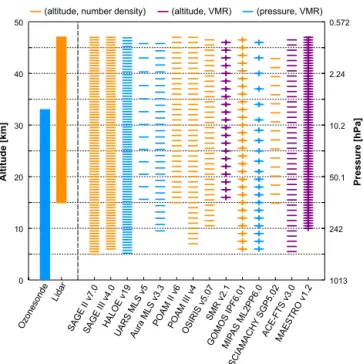
Figure 1.Overview of the native representation of the ozone profile records (see legend). A vertical band defines the approximate range for the ground-based data sets, while individual levels are shown for satellite profiles. Only the levels considered in our analyses are de-picted. Profile-dependent vertical grids are marked with small ver-tical bars. Differences between geometric and geopotential height are neglected.
UARS and Aura MLS) is typically more reliable and there-fore used as native vertical scale instead of altitude.
We screen the satellite profiles according to the prescrip-tions of the data provider (Table 3). In some cases this im-plies the removal of a considerable part of the data record, e.g. periods during which the product stability is not guar-anteed. In particular, we remove the UARS MLS data af-ter the 15 June 1997 switch-off of the 63 GHz radiome-ter (Livesey et al., 2003). We also reject MIPAS observations before January 2005 since these are potentially biased rel-ative to those from the second phase of the mission due to a different set of retrieval microwindows (Ceccherini et al., 2013). Finally, from September 2010 onwards the ACE-FTS and MAESTRO retrievals are affected by problems with aux-iliary input data and therefore rejected from the analysis. These issues were fixed in the v2.5/v3.5 data release of ACE-FTS, which extends the mission’s record to the present. Data providers generally recommend a vertical range for their ozone product in addition to the standard screening prescrip-tions, see Table 3. Here, we keep all grid levels in order to verify at what point the data quality starts to degrade. Fig-ure 1 shows for each instrument the vertical range considered in this work.
Each record is provided in its native ozone profile repre-sentation (Fig. 1) defined by the vertical coordinate (altitude
or pressure), the vertical grid levels and the quantity in which ozone is expressed (volume mixing ratio, VMR, or num-ber density). The vertical grid of some records varies with the changing tangent heights of the measurements. Through-out this work the difference between geometric altitude and geopotential height is neglected. Satellite data providers typ-ically include the pressure and/or temperature data required to convert the native ozone profiles to another representation. These auxiliary data are sometimes retrieved by the same processor but in general taken from an external source (see Table 3). This assessment focuses primarily on data quality in the satellite’s native profile representation. But given its importance in, e.g. the data merging context we complement the analysis with tests of the impact of auxiliary data on the profile quality in other representations. We will see in Sect. 6 that this should indeed not be ignored.
3 Analysis approach and data preprocessing
A careful design of the analysis allows us not only to obtain robust estimates of the data quality of the individual satellite records but also, and this is one of our primary objectives, to assess their mutual consistency. Prerequisite to achieving these goals is a good understanding of the metrological as-pects of the comparison analysis. Our analysis approach is therefore based on three principles that reduce confounding methodological biases. First of all, we use a single analy-sis and software framework. Second, all satellite records are compared to the same reference data, from ground-based ob-servations. And finally, the manipulation of satellite data is kept to a strict minimum. In this section we describe the general aspects of the analysis. A detailed account of how decadal stability, bias and short-term variability are estimated follows in Sects. 4 and 5.
The ozonesonde and lidar networks provide vertical ozone profiles of well-documented quality and serve as suitable transfer standards on a pseudo-global scale and from the tro-posphere to the stratopause. We compare the satellite profiles to co-located ground-based measurements in relative units
1xij(l)=100×
xij,sat(l)−x′ij,gnd(l)
xij,′ gnd(l) . (1)
Here,xij,sat(l)andxij,′ gnd(l)represent respectively satellite
and (vertically smoothed and representation-transformed) ground-based ozone at grid levell of co-location pairi for correlative instrumentj. If the satellite bias is of multiplica-tive nature2then any time dependence in ozone levels (e.g. seasonal, interannual, solar cycle) is divided out in the rela-tive differences. Another advantage is that it allows for a di-rect comparison between the results in different ozone quan-2A set of observations{x}contains a multiplicative bias with
tities. A disadvantage, however, is that relative differences are sensitive to low ozone values, leading to larger values in and below the UTLS (upper troposphere lower stratosphere) and in the upper stratosphere.
1xis determined by several factors besides pure measure-ment and retrieval uncertainties (Sxsat,Sxgnd) because satel-lite and ground-based instruments have different perceptions of a variable atmosphere. Vertical and horizontal resolutions differ and the probed air masses rarely coincide perfectly in space and time. In addition, the comparison can only be done when both profiles are expressed in the same representation. As a result, the total comparison error budget contains terms related to the differences in smoothing, the spatiotemporal mismatch of the co-locations and the auxiliary data used to transform between profile representations. When correla-tions between the terms are disregarded, the total uncertainty covariance matrix (including systematic and random compo-nents) becomesS1x=Sxsat+Sxgnd+Ssmoothing+Smismatch+ Sauxiliary(von Clarmann, 2006). Furthermore, when1xdata are averaged or regressed the co-located profile sample may not be sufficiently representative of the actual state of the studied parameter (ozone differences). Toohey et al. (2013) recently showed the importance ofSsamplingfor trace gas cli-matologies and Damadeo et al. (2014) for time series analy-ses. Estimating sampling uncertainty for validation purposes is an analysis in its own right and outside the scope of this paper.
The next few paragraphs describe the data preprocess-ing scheme in which the mitigation of the uncertainties due to differences in smoothing, geolocation and auxiliary data plays a central role. Preprocessing starts off by removing the unreliable measurements following the guidelines of the data providers. Table 3 lists the recommended screening procedure references for the satellite records. Ground-based data are filtered using general criteria, removing measure-ments with larger uncertainties: altitudes above the 5 hPa level (∼33 km) for ozonesondes and outside the 15–47 km range for lidars. In addition, we reject measurement levels with clearly unphysical readings (O3<0, p <0 hPa, T < 0 K or T >400 K) or during unrealistic jumps in pressure (dp/dt >0 and dz >0.1 km). Entire profiles are discarded from further analysis when (a) more than half of the levels are tagged bad, or (b) less than 30 levels are tagged good.
The choice of a co-location window is a trade-off between mismatch uncertainties and a sufficiently large sample size to obtain robust statistical estimates. We found that a maxi-mum horizontal distance1rof 500 km between the profiles is optimal, given the typical horizontal resolution of the order of a few hundred km of the satellite and ground-based mea-surements. The maximal temporal separation 1t is 6 h for MIPAS and Aura MLS, and 12 h for the other instruments. When multiple satellite profiles are present in the co-location window around a ground-based profile, only the pair closest in space and time is retained, defined byq1r2+Vwind2 1t2
withVwind=100 km h−1 as a rough estimate of horizontal
wind speed in the stratosphere. Multiple co-locations occur mostly between polar orbiting instruments and high latitude stations. Figure S1 in the Supplement shows the latitude– time cross-section of the co-location samples.
Mismatch uncertaintiesSmismatchincrease when and where atmospheric inhomogeneities are larger. Diurnal variations in ozone contribute a systematic component since the lo-cal time of ground-based observations (ozonesonde mostly around noon, lidar during night) and satellite measurements (Table 3) is generally constant. Biases due to the diurnal cy-cle are negligible below 30 km, but not at higher altitudes where ozone reaches minimal levels after dawn and max-imal values in the afternoon (Schanz et al., 2014; Parrish et al., 2014; Sakazaki et al., 2015). The largest effect on our bias estimates is expected in the middle (< 2–3 %) and upper stratosphere (< 4 %) for the comparisons of lidar to sunset occultation profiles and, to a lesser extent, to the evening ob-servations by SMR and OSIRIS. The random component of mismatch uncertainty is typically 5 % but can reach 20 % at, e.g. Antarctic stations dropping in and out of the polar vor-tex (Cortesi et al., 2007; De Clercq, 2009).
profiles in many satellite records for this purpose. As we have seen in Sect. 2.2, these auxiliary data originate from differ-ent sources which may lead to a represdiffer-entation-dependence of the mutual consistency of the satellite data quality. This is discussed further in Sect. 6. Until then, only the correl-ative data are converted when needed. Ozonesonde data are transformed with the help ofpandT measurements from the attached radiosonde, and lidar data using ERA-Interim fields. The quality of these ancillary data has been investigated by various authors (e.g. Sun et al. (2013); Stauffer et al. (2014); Simmons et al. (2014); Inai et al. (2015)). The regridding to the satellite’s vertical grid is based on a pseudo-inverse in-terpolation method (Calisesi et al., 2005). Since the ground-based grid is more finely resolved than the satellite grid, the associated regridding uncertainties are generally negligible. We note that the SMR, GOMOS, MIPAS and MAESTRO profiles are inevitably regridded as well because the grid is variable. In these cases the levels of the comparison grid are selected to reflect the average spacing between two lines of sight.
To conclude this section we repeat the importance of using a single analysis and code framework. Apart from some un-avoidable preprocessing steps, the data and analysis flow is identical for all 14 satellite comparison studies. In this way, the methodological biases are mostly identical and, hence, unlikely responsible for eventually observed differences be-tween the satellite records. This approach will be exploited in Sect. 7. The next two sections present a detailed assess-ment of the bias, the short-term variability and the decadal stability of each individual satellite record.
4 Decadal stability
We estimate the decadal stability of satellite data through a robust analysis of the time series of the satellite-ground dif-ferences. This is a two-step process, in which the linear drift is first estimated at each ground station and subsequently av-eraged over the ozonesonde and lidar networks. The focus of this section is on the decadal stability of the individual satel-lite records, in their native profile representation. Later on we expand the discussion to the consistency of drift between profile representations (Sect. 6) and between satellite records (Sect. 7).
4.1 Methodology
4.1.1 Time series analysis at individual stations
We first estimate the drift of the satellite data at each ground station. The comparison time series can contain large gaps and/or outliers; see, e.g. the GOMOS comparisons in Fig. 2 (top panel). Hence robust techniques are needed to estimate not only the drift but also its uncertainty (Muhlbauer et al., 2009; Croux et al., 2004). To this end we use an iterative Tukey-bisquare reweighted least-squares procedure to fit the
daily averaged relative difference time series to a linear re-gression model
1xij(l)=αj(l) (ti−t0)+βj(l)+eij(l). (2)
With 1xij(l) as in Eq. (1) at timeti and grid level l, and
the fit residualeij(l). In this model, the fit parameter αj(l)
represents the linear drift of the satellite data relative to the ground-based record j, whereas βj(l) is the bias between
both records at reference timet0. Time series with less than 10 data points are not regressed. The significance of the es-timatedα(l)ˆ is tested using a robust estimate of its standard
deviationσˆα(l) proposed by Street et al. (1988), a slightly
modified version of the ordinary least-squares expression. Figure 2 illustrates three time series with superimposed re-gression results (left panels, blue line) and the correspond-ing 95 % confidence intervals forα(l)ˆ (right panels, vertical
dashed blue lines).
4.1.2 Aggregation into ground network average In a second step, the drift estimatesαˆj(l)are averaged over
various ground stationsj = {1, . . ., N}. None of the satellite
records exhibit a clear latitudinal structure of drift (see, for instance HALOE and Aura MLS at 25 km in Fig. 3). There-fore, we average the results over the entire sonde network and over the entire lidar network. Since there is a clear vari-ability in the regression uncertainty across the network, each station estimate is weighted by the inverse of its variance wj(l)= ˆσα,j−2(l). The network-averaged drift
¯
α(l)= P
jwj(l)αˆj(l)
P
jwj(l)
, (3)
has a standard deviationσα¯(l)=1/
qP
jwj(l).
The single-site drift uncertainties alone do not always explain the observed variability of the drift estimates over the network. When the number of stations is large enough
(N&20) the distribution of normalised residuals νj(l)=
(αˆj− ¯α)/σˆα,jshould have unit variance for realistic estimates ˆ
σα of the variance of α. That is typically not the case forˆ
the dense samplers, that tend to have larger variance as il-lustrated, for instance, for Aura MLS in Fig. 3 (right). This suggests an unaccounted-for source of uncertainty, likely re-lated to differences in sampling or inhomogeneities across the ground-based network. We follow an ad hoc approach to incorporate this unknown component, by scaling the uncer-tainty up
σα¯∗(l)=κ(l)×σα¯(l) (4)
so that the reducedχ2(l)=qN1−1P
jνj(l)2becomes unity.
We also assume, conservatively, that the original regres-sion uncertainty does not overestimate the true uncertainty; henceκ(l)=max
(SA
T/GND) - 1 [%]
z=37.6 km
Baseline: -9.3±3.4 %/dec, Monthly: -6.7±4.2 %/dec, Harmonic: -9.3±3.3 %/dec
2002 2003 2004 2005 2006 2007 2008 2009 2010 2011 2012 2013
-25 -20 -15 -10 -5 0 5 10 15 20 25
Number of bootstrap samples
-15 -10 -5 0 5 10 15 0
50 100 150
(SA
T/GND) - 1 [%]
z=42.5 km
-25 -20 -15 -10 -5 0 5 10 15 20 25
Number of bootstrap samples
0 20 40 60 80 100
Baseline: +11.6±4.6%/dec, Monthly: +13.7±6.0 %/dec
(SA
T/GND) - 1 [%]
z=19.5 km
-25 -20 -15 -10 -5 0 5 10 15 20 25
Number of bootstrap samples
0 20 40 60 80 100
Baseline: -4.1±5.7 %/dec, Monthly: -3.9±8.7 %/dec GOMOS IPF6.01 vs. Payerne sonde (46.8° N, 7.0° E)
OSIRIS v5.07 vs. OHP lidar (43.9° N, 5.7° E)
SCIAMACHY SGP5.02 vs. Lauder lidar (45.0° S, 169.7° E)
Drift [% dec ]-1
Figure 2.(Left) Time series of the ozone comparisons for GOMOS vs. Payerne ozonesonde at 19.5 km (top), for OSIRIS vs. OHP lidar at 42.5 km (centre), and for SCIAMACHY vs. Lauder lidar at 37.6 km (bottom). A 1-year running median filter is applied to highlight long-term dependence (white line and 1σ shaded area). The blue line depicts the baseline regression model, while the green and orange lines show cross-checks (see text). The estimated driftαˆ and its 1σˆα uncertainty is mentioned at the bottom of each panel. (Right) Distribution of the
drift obtained from 2500 bootstrapped samples of the time series on the left. The light red zone marks the 95 % interpercentile of the drift distribution, which should be compared to the analytic expressionαˆ±2σˆα(vertical blue lines).
standard deviation σα¯∗(l) is used to test the significance of the drift averages at the 5 % level. Figure S2 shows theκ -adjustment factor for each satellite record.
4.1.3 Sensitivity to analysis parameters
The importance of correct single station uncertaintiesσˆα,j(l)
is evident for the calculation of both the weighted mean and its uncertainty. The possible presence of data gaps, outliers and auto-correlation in the time series led us to cross-check the analytic expression of Street et al. (1988) with a boot-strapping technique (Efron and Tibshirani, 1986). Each com-parison time series was resampled 2500 times by replace-ment of single data points, and subsequently regressed to re-construct the distribution ofαˆj(l)(Fig. 2, right). The 2.5 and
97.5 % quantiles define the 95 % confidence interval (light red area) which is in good agreement with the analytic ex-pression (vertical dashed blue lines). Replacing the analytic by the bootstrap-derived uncertainties in Eqs. (3) and (4)
changesα¯ andσα¯∗ typically by less than∼0.5 % decade−1
(Fig. S3). Figure 2 (left) also illustrates the outcome of other sensitivity checks, such as changing the temporal resolution of the time series prior to regression (from daily to monthly, green curve) or adding a 1-year harmonic component to the regression model (orange curve). Again, the results are very consistent, changingα¯ and σα∗¯ typically by less than
∼1 % decade−1 (Fig. S3). These cross-checks demonstrate
the robustness of the results to changes in the analysis pa-rameters.
4.2 Selection of ground sites
-20 -15 -10 -5 0 5 10 15 20
Number of sonde stations
0 1 2 3 4 5 25.1 hPa 10/1991–11/2005
Latitude [deg]
-90 -60 -30 0 30 60 90
-20 -15 -10 -5 0 5 10 15 20
Normalised residual ν
Number of sonde stations
-4 -3 -2 -1 0 1 2 3 4 0
2 4 6 21.5 hPa
Aura MLS v3.3 vs. ozonesonde / lidar
HALOE v19 vs. ozonesonde / lidar
Drift [% dec ]
-1
Drift [% dec ]
-1
8/2004–5/2013
Figure 3.(Left) Driftαˆj and one sigma uncertaintyσˆα,j of HALOE (top) and Aura MLS (bottom) around 25 km relative to co-located
observations at each station in the NDACC/GAW/SHADOZ ozonesonde (black) and NDACC lidar (blue) networks. Also shown are the weighted mean for the ozonesonde networkα¯ (horizontal white line), its adjusted uncertaintyσα∗¯ (dark grey area) and the standard deviation of the ensemble of single sonde site drift estimates (light grey area). (Right) Corresponding distribution of normalised residualsνfrom the ozonesonde network.
stations with a short data record or with episodic observa-tions collected during field campaigns are not retained for the regression analyses. Figure 4 shows the vertical drift pro-files for seven limb/occultation records at nine NDACC lidar sites, six of which were also studied by Nair et al. (2012). The common vertical drift structure of the sounders noted at Andøya and Tsukuba is indicative of features in the lidar time series, which may influence the network-averaged satel-lite drift analyses. Both lidar sites are therefore rejected from the stability analysis. Also the Dumont d’Urville compari-son time series are not considered, for two reacompari-sons. First, the lidar system was entirely redesigned in 2002 (David et al., 2012), which possibly introduces inhomogeneities in the time series. And secondly, the station is located close to the edge of the polar vortex, which can induce spurious bi-ases due to mismatches in the air parcel sampled by lidar and satellite. The latter challenge could be overcome, e.g. by co-locating in equivalent-latitude space (Bergeret, 1999), but this was outside the scope of this work. The drift results at Hohenpeißenberg for all recent sounders are significantly negative above about 25 km, while the results scatter around zero for two historic occultation instruments. Inspection of the time series indeed showed that the Hohenpeißenberg li-dar reported more ozone for a few years after 2007 (Nair et al., 2012). This station is hence discarded from the drift analyses of all satellite sounders operational during and
af-ter 2007 (Table 3). Similarly, the Table Mountain lidar (Mc-Dermid et al., 1990) measured higher ozone relative to satel-lite instruments during 2007–2008. This bias disappeared in later years to leave the satellite drift estimates nearly un-changed (Nair et al., 2012). One exception is Aura MLS since the temporary lidar bias occurred close to the start of the mis-sion. Nonetheless, we keep the Table Mountain lidar data for our analyses. A similar procedure was followed to dis-card about 20 ozonesonde records. For one satellite instru-ment we deviate from previous, standard selection of ground sites. SCIAMACHY drift results in the Arctic are very dif-ferent from those in the rest of the atmosphere, especially for lidar. We believe this is a combined result of sampling and the seasonal cycle observed in the difference time series (Sect. 5). Therefore, all Arctic stations are excluded from the drift analysis of SCIAMACHY. Tables 1 and 2 list the sta-tions used for the drift analysis (last column). Thanks to the pseudo-global coverage of the ozonesonde network, the net-work average should be a reasonably robust representation of the global satellite drift. Lidar network averages, on the other hand, are less representative of the global state and they are somewhat more sensitive to the station selection as well.
Altitude [km]
15 20 25 30 35 40 45
Pressure [hPa]
2
5
10
20
50
100
Altitude [km]
15 20 25 30 35 40 45
Pressure [hPa]
2
5
10
20
50
100
Altitude [km]
-15 -10 -5 0 5 10 15 15
20 25 30 35 40 45
-15 -10 -5 0 5 10 15 -15 -10 -5 0 5 10 15
SAGE II v7.0
HALOE v19
OSIRIS v5.07
GOMOS IPF6.01
MIPAS ML2PP6.0
SCIAMACHY SGP5.02 Aura MLS v3.3
Pressure [hPa]
2
5
10
20
50
100 Eureka (80° N, 86° W) Ny-Ålesund (79° N, 12° E) Andoya (69° N, 16° E)
Hohenpeißenberg (48° N, 11° E) OHP (44° N, 6° E) Tsukuba (36° N, 140° E)
Table Mountain (34° N, 118° W) Mauna Loa (20° N, 156° W) Lauder (45° S, 170° E)
Drift α [% dec ]-1 Drift α [% dec ]-1 Drift α [% dec ]-1
Figure 4.Comparison of the vertical structure of the driftαof two historic (dashed lines) and five recent (solid) satellite records relative to stratospheric lidar observations at nine NDACC stations. The shaded area represents the unadjusted 68 % confidence interval, which does not include possible uncertainties from differences in sampling or from inhomogeneities in the lidar network. The analysis is performed in the native profile representation of each satellite record.
(< 0.5–1 % decade−1) for SCIAMACHY due to its peculiar data characteristics in the Arctic. Lidar network averages are more sensitive to the selection of sites, especially for the recent satellite records. They differ by 1–2 % decade−1 above 25 km, mainly as a result of the inclusion of the Ho-henpeißenberg data which systematically pulls the vertical drift profile towards more negative values. The impact of lidar site selection is much smaller for older records, less than 0.5 % decade−1. Also the estimates of drift uncertainty are somewhat affected, but not as much as the actual drift values. Typically, the difference in uncertainty is less than 0.5 % decade−1. Later on, we describe the remarkable agree-ment between the ozonesonde and lidar-derived drift results, strengthening the confidence in the stability of these ground networks (Fig. 5).
4.3 Results
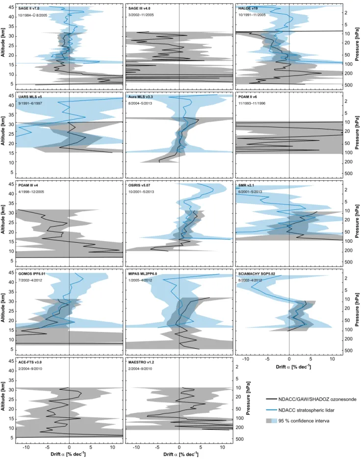
Below we report on the vertical structure of the network-averaged drift estimates and their significance for each satel-lite record. We also mention some indicators of the per-formance of the ground networks for this type of analysis: (a) the smallest value of the 1σ regression uncertainty found across the network, (b) the typically found uncertainty and (c) the adjustment factor κ. Main results are presented in Fig. 5 and summarised in Table 4.
4.3.1 SAGE II
net-NDACC/GAW/SHADOZ ozonesonde
NDACC stratospheric lidar
95 % confidence interval
-10 -5 0 5 10 -10 -5 0 5 10
-10 -5 0 5 10
Altitude [km]
5 10 15 20 25 30 35 40 45
Altitude [km]
5 10 15 20 25 30 35 40 45
Altitude [km]
5 10 15 20 25 30 35 40 45
Altitude [km]
5 10 15 20 25 30 35 40 45
Altitude [km]
5 10 15 20 25 30 35 40 45
Pressure [hPa]
2
5
10
20
50
100
200
500
Pressure [hPa]
2
5
10
20
50
100
200
500
Pressure [hPa]
2
5
10
20
50
100
200
500
Pressure [hPa]
2
5
10
20
50
100
200
500
Pressure [hPa]
2
5
10
20
50
100
200
500
SAGE II v7.0 SAGE III v4.0
3/2002–11/2005
HALOE v19 10/1991–11/2005
UARS MLS v5 9/1991–6/1997
Aura MLS v3.3 8/2004–5/2013
POAM II v6 11/1993–11/1996
POAM III v4 4/1998–12/2005
OSIRIS v5.07 10/2001–5/2013
SMR v2.1 6/2001–5/2013
GOMOS IPF6.01 7/2002–4/2012
MIPAS ML2PP6.0 1/2005–4/2012
SCIAMACHY SGP5.02 8/2002–4/2012
ACE-FTS v3.0 2/2004–9/2010
MAESTRO v1.2 2/2004–9/2010 10/1984–Ü 8/2005
Drift α [% dec ]-1
Drift α [% dec ]-1 Drift α [% dec ]-1
Table 4.Overview of the drift of satellite ozone profile records relative to ozonesonde and lidar, in the lower, middle and upper stratosphere. For each altitude region we present the range of the network average of the drift (α¯) and its adjusted one sigma uncertainty (σα∗¯). Bold values indicate results with more than 2σsignificance.
Drift SAT-GND 10–20 km 20–30 km 30–45 km Remark
[%/decade] α¯ 1σα¯∗ α¯ 1σα∗¯ α¯ 1σα∗¯
SAGE II [−3,−1] 1–3.5 [−2,0] 0.5–1 [−2,+2] 1–3 very stable
SAGE III [−15,−2] 5–15 [−10,0] 3–6 no results record too short
HALOE [−3,+5] 1.5–6 [–7, –1] 1–2 [−5,0] 1.5–6 significant 20–30 km
UARS MLS no UARS MLS data [−1,+5] 2–4 [−2,+3] 3–12 record short
Aura MLS [−4,0] 0.8–1.5 [0,+3] 0.5–1 [−1,+3] 1–6 very stable
POAM II no results [−15,+15] 9–20 no results record too short
POAM III [−4,+10] 2–10 [−8,−2] 2–4 no results record sparse
OSIRIS [−5,+1] 1–4 [+1,+3] 0.8–1 [+1, +8] 1–2.5 significant 36–44 km,
indi-cations 25–34 km
SMR no SMR data [−3,+5] 1.5–3 [−15,+3] 3–10 indications > 35 km
GOMOS [−12,−3] 2–20 [−4,−1] 1.5–2.5 [−1,+3] 1.5–4 indications 15–25 km
MIPAS (OR) [−1,+3] 1–2 [0,+3] 1–2.5 [−4,+1] 2.5–5 stable
SCIAMACHY [0,+4] 1–2.5 [+1,+3] 0.8–1.5 [–9, +1] 1–5 significant 32–42 km,
indi-cations < 30 km
ACE-FTS [−5,0] 3–7 [−4,+3] 2.5–3.5 no results record sparse
MAESTRO [−7,+10] 3–12 [0,+6] 3–4 no results record sparse
works is, respectively, 0.8 % decade−1 and 1.6 % decade−1. The average drift uncertainty over the ensemble of stations is ∼4 % decade−1. The drift results are furthermore very consistent from one station to another, with a spread of 2–3 % decade−1at 25 km (Fig. 4). The sonde and lidar de-rived estimates are statistically consistent as well. When aggregated over the entire ground network a significant SAGE II drift should be detectable at the 1–2 % decade−1 level, depending on altitude.
In the middle and upper stratosphere, between 20 and 40 km, the average drift is slightly negative ex-cept around ∼33 km (Fig. 5). The negative drift remains
smaller than 1–2 % decade−1and is not significant. At lower altitudes the drift becomes gradually more pronounced, but is never significant either as a result of the increased atmospheric variability or noise in the SAGE II record. We therefore conclude that the SAGE II record is stable relative to the ground measurements, at least within 2 % decade−1. 4.3.2 SAGE III
SAGE III collected data for only 3.5 years, which excludes the upper stratosphere from our study as no lidar sites provide sufficient statistics. Between 20 and 30 km the minimal drift uncertainty is 6 % decade−1, while that of most stations is easily twice as high.
SAGE III ozone decreases relative to ground measure-ments, by 2–6 % decade−1 in the middle stratosphere (MS) and more than 10 % decade−1 at lower altitudes (Fig. 5). The significance is by far insufficient however for a 2σ detection. The detection limit for the network-averaged drift is at best 6 % decade−1 between 20 and 30 km. In
the lower stratosphere (LS) the threshold rapidly worsens to 10–30 % decade−1 due to the increased contribution of noise from natural variability and instrumental noise. We therefore conclude that SAGE III is stable within about
±10 % decade−1, which is consistent with an earlier report by Wang et al. (2006).
4.3.3 HALOE
The 14-year HALOE record allows for a quite detailed study of the stability as well. The typical uncertainty at single sta-tions is 5 % decade−1, which is comparable to the variabil-ity of the spread between stations (Fig. 3, top left, light grey band). The 2σdetection threshold for the network average is 2–3 % decade−1or more.
For altitudes above 100 hPa we observe a negative drift of about 1–7 % decade−1 (Fig. 5). The result is significant between 10 and 40 hPa for both the ozonesonde and the li-dar comparisons. Figure 3 demonstrates that negative drifts are found across the entire ground network (left panel), all centred around the network-averaged value (right). At alti-tudes above 10 hPa and below 40 hPa the drift is less than
±5 % decade−1with an uncertainty of 1.5–6 % decade−1and
hence not significant. No dependence on vertical coordinate or ozone quantity was found for the HALOE drift results (Fig. 9), so these cannot be explained by drifting auxiliary data of the correlative records (Sect. 6).
obtain a significant result already at the 2–3 % decade−1level between 10 and 50 hPa. Our result is consistent with the earlier reports, although a direct comparison is not straight-forward due to the different timespan and vertical coordi-nate (we come back to this in Sect. 6). From Fig. 5 we infer that the middle stratospheric drift of HALOE rela-tive to SAGE II must range between 0 and−5 % decade−1, which is comparable in sign and in magnitude with the−(0– 10) % decade−1reported by Morris et al. (2002, Fig. 4a) and −(2–4) % decade−1by Nazaryan et al. (2005, Fig. 8).
4.3.4 UARS MLS
The UARS MLS record is somewhat short (less than 6 years) which limits the drift study especially at low altitudes and relative to the lidar instruments. Between 5 and 50 hPa (20–35 km) the single station drift uncertainty is 5 % decade−1at best, but typically twice as large. When the results are averaged over the ground network the 2σ de-tection threshold is 4–8 % decade−1. At other altitudes the threshold increases rapidly, by a factor of at least 2.
For altitudes below 10 hPa the ozonesonde comparisons show a non-significant positive drift of 0–3 % decade−1 (Fig. 5). The drift relative to lidar, on the other hand, is nega-tive but it is also not well constrained. As a result, the differ-ence between the sonde- and lidar-derived results is not sig-nificant. In fact, it is difficult to conclude anything from the lidar results; the results at different sites tend to be somewhat inconsistent, especially at altitudes above the 10 hPa level. While the upper stratospheric drift of UARS MLS goes up to +10 % decade−1 relative to the Observatoire de
Haute-Provence (OHP) and Table Mountain lidars, it goes down to −10 % decade−1 relative to the Mauna Loa and Lauder
lidars. This necessitates a large χ2-adjustment of κ≃2.5 for lidar (Eq. (4) and Fig. S2) and results in a final uncer-tainty of about 10 % decade−1. We conclude that between 10 and 50 hPa the UARS MLS instrument is stable within about±5–10 % decade−1, perhaps slightly worse. In the up-per stratosphere the discrepancy between the lidar results is too large to assess the stability of UARS MLS.
We also note a dependence of the UARS MLS ozone drift results with profile representation due to an ascending drift in the accompanying GPH profile products (Fig. 9). More details and a recommendation to avoid such representation-dependences follow in Sect. 6.
4.3.5 Aura MLS
The stability of the Aura MLS instrument can be studied in great detail, thanks to its excellent temporal and spa-tial sampling. Single site drift uncertainty is at best 0.6 and 2 % decade−1on average. Regression uncertainties are sub-stantially smaller than the observed standard deviation of the drifts over the network, which is about 4–6 % decade−1 at altitudes above 50–100 hPa (Fig. 3, bottom). This leads to a
considerableχ2-adjustment (Fig. S2) ofκ≃2.5 in the
mid-dle stratosphere (sonde) andκ≃3 in the upper stratosphere
(lidar). The resulting 2σdetection limit for network averages is 1–3 % decade−1 at altitudes below 5 hPa, and increases rapidly in the uppermost stratosphere.
In the upper and middle stratosphere the average drift is slightly positive, but generally not more than 1.5– 2 % decade−1 (Fig. 5). Sonde and lidar derived results are very consistent. A significant negative drift seems to de-velop at altitudes below 100 hPa, which we think is due to an underestimation of the uncertainty. Indeed, obtaining re-alistic uncertainties at the level of a few % decade−1 level in the UTLS is a daunting task. We therefore conclude that Aura MLS v3.3 is stable in the entire stratosphere, certainly within 1.5 % decade−1 (MS) and 2 % decade−1 (US). Our ground-based estimates are consistent with earlier intercom-parisons of Aura MLS, MIPAS (Eckert et al., 2014) and OSIRIS (Adams et al., 2014), indicating drifts between the instruments less than±3–5 % decade−1.
We will see later on that the above drift results differ from those in non-native vertical coordinate representations, due to an overall descending drift of the Aura MLS GPH profiles (Fig. 9). This issue and a possible solution will be discussed in Sect. 6.
4.3.6 POAM II
The analysis of POAM II is extremely limited due to its infrequent sampling and short record, merely 3 years. The regression requirement of at least 10 data points was met at just 7 polar ozonesonde stations. There were not enough co-locations with lidar instruments to study the up-per stratosphere. Drift uncertainty is about 30 % decade−1 at most sites and 20 % decade−1 in the best case. The re-sulting 2σ detection threshold for the network average is 20–40 % decade−1 in the middle stratosphere. This is much larger than the observed drifts, which range from
−15 % decade−1at 20 km and 30 km to+15 % decade−1at 25 km (Fig. 5). We conclude that the stability of POAM II is better than±25 % decade−1in the middle stratosphere.
4.3.7 POAM III
20 and 30 km, at a rate of −(2–8) % decade−1 (Fig. 5). At
lower altitudes the drift changes sign. None of our results are statistically significant. We conclude that POAM III is sta-ble within, respectively,±5 and 15 % decade−1in the middle and lower stratosphere.
4.3.8 OSIRIS
The OSIRIS time series are densely sampled at many ground stations. In the middle and upper stratosphere the minimum drift uncertainty is 1.3 % decade−1and typically amounts to 3–4 % decade−1. The regression uncertainties do not fully explain the observed variability of 5–6 % decade−1between stations above 20 km. The correspondingχ2-adjustment fac-torκ is∼1.5–2 for the sonde network and mostly less than
1.5 for the lidar network. The 2σ detection limit for the net-work average is 3 % decade−1at 15 km, 1.6 % decade−1 be-tween 20 and 30 km and 5 % decade−1at 45 km.
In the lowermost stratosphere the OSIRIS drift rel-ative to correlrel-ative measurements is negrel-ative, at most
−5 % decade−1 and not significant (Fig. 5). There are clear indications of a positive drift between 15 and 35 km, of about 1–3 % decade−1. While the sonde-derived result is signifi-cant (> 22 km), that is generally not the case for the lidar results (except between 28 and 34 km). In the upper strato-sphere the positive drift becomes more pronounced and very significant above 37 km. Its presence is easily visible in the comparison time series, e.g. at the OHP lidar (Fig. 2). Around 42 km we find a > 2σ drift of+8 % decade−1at three of the
four best sampled lidar stations (Fig. 4). Adams et al. (2014) reported a +(3–6) % decade−1 drift of OSIRIS relative to
Aura MLS in the US, depending on how the Aura MLS data (pressure-VMR) are converted to the native OSIRIS sys-tem (altitude-number density). This is consistent with the 5 % decade−1difference that we find between our lidar-based drift estimates for these two instruments. Also Rahpoe et al. (2015) obtained positive drift estimates of OSIRIS relative to five satellite instruments above 40 km, though the results are not significant for most instrument pairs.
In summary, OSIRIS ozone drifts very likely to higher val-ues above 20 km. The drift is quite small up to 35 km and close to the 5 % significance threshold. In the upper strato-sphere the presence of a+(5–8) % decade−1drift is evident.
The OSIRIS team has found that the drift in ozone may be caused by a positive drift in the altitude registration. Efforts are under way to correct for this in the next data release. 4.3.9 SMR
Even though the SMR record spans 12 years and has good sampling properties, the ability to assess its stability is lim-ited by the noise of the profiles. In Sect. 5 we show that the single SMR profile noise exceeds 20 % in the tropics and 30 % at higher latitudes. This is substantially larger than for any other satellite record in this study. As a result,
the drift uncertainty is at best 5–6 % decade−1and typically ∼10 % decade−1at individual ground sites. The regression
uncertainties cover the observed drift variability across the ground network, so theχ2-adjustment is close to one. In the end, the 2σthreshold to detect averaged drifts ranges from 3 to 10 % decade−1between 25 and 40 km.
The SMR profile drifts slightly to higher values in the mid-dle stratosphere, although by no more than+5 % decade−1 which is insignificant (Fig. 5). Above 30 km the drift changes sign and increases rapidly in magnitude, reaching
−12 % decade−1 around 40 km. Due to the large
single-profile noise the negative drift is only significant at 2σ level between 40 and 43 km. A recent six-satellite intercompari-son study pointed to a negative drift of SMR upper strato-spheric ozone as well, though the estimates were generally not considered significant (Rahpoe et al., 2015). These re-sults contrasts with satellite intercomparisons by Jones et al. (2009) which indicated an insignificant positive drift of SMR relative to a multi-satellite average in the upper stratosphere. The difference may be due to a shorter period (2001–2007) or due to the different data versions, and deserves further study. Meanwhile, we conclude that SMR is stable within
±6–8 % decade−1over most of the stratosphere. SMR ozone trends in the uppermost stratosphere, however, should be in-terpreted cautiously as they possibly underestimate the actual trend by more than 10 % decade−1.
4.3.10 GOMOS
The constraints on the stability of GOMOS are weaker than for its contemporary limb sounders, due to its sparser sam-pling and, below ∼20 km, its larger noise. These
limita-tions are clear from the comparison time series at the Pay-erne ozonesonde station (Fig. 2). In the middle stratosphere, the drift variability between stations is about 10 % decade−1, which is larger than the uncertainties at individual sites, about 3 % decade−1at best and 7 % decade−1in general. The χ2-adjustment increases the uncertainty of the network av-erages byκ≃1.5. The resulting 2σ detection threshold is 3–5 % decade−1between 20 and 40 km and raises rapidly in the lower stratosphere, e.g. to∼12 % decade−1at 15 km.
In the upper stratosphere the lidar results are scattered, but they point on average to a small, positive drift of GO-MOS retrievals above 35 km (Fig. 4). The maximum drift is only+3 % decade−1at 45 km, well below the 2σ thresh-old. However, below 25–30 km a pronounced negative drift develops with decreasing altitude, from −1 % decade−1 at
30 km to−4 % decade−1at 20 km (Fig. 5). The results for the


![Table Mountain (34° N, 118° W) Mauna Loa (20° N, 156° W) Lauder (45° S, 170° E) Drift α [% dec ]-1 Drift α [% dec ]-1 Drift α [% dec ]-1](https://thumb-eu.123doks.com/thumbv2/123dok_br/18322488.349933/13.918.90.683.97.698/table-mountain-mauna-loa-lauder-drift-drift-drift.webp)