PARALLEL PROCESSING OF BIG POINT CLOUDS USING Z-ORDER-BASED
PARTITIONING
C. Alis∗, J. Boehm, K. Liu
Dept. of Civil, Environmental and Geomatic Engineering, University College London, Gower Street, London, UK [email protected]
Commission II, WG II/2
KEY WORDS:Z-order, Spatial partitioning, Big Data, LiDAR, Point Cloud, Apache Spark
ABSTRACT:
As laser scanning technology improves and costs are coming down, the amount of point cloud data being generated can be prohibitively difficult and expensive to process on a single machine. This data explosion is not only limited to point cloud data. Voluminous amounts of high-dimensionality and quickly accumulating data, collectively known as Big Data, such as those generated by social media, Internet of Things devices and commercial transactions, are becoming more prevalent as well. New computing paradigms and frameworks are being developed to efficiently handle the processing of Big Data, many of which utilize a compute cluster composed of several commodity grade machines to process chunks of data in parallel.
A central concept in many of these frameworks is data locality. By its nature, Big Data is large enough that the entire dataset would not fit on the memory and hard drives of a single node hence replicating the entire dataset to each worker node is impractical. The data must then be partitioned across worker nodes in a manner that minimises data transfer across the network. This is a challenge for point cloud data because there exist different ways to partition data and they may require data transfer.
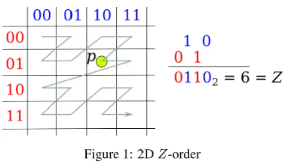
We propose a partitioning based onZ-order which is a form of locality-sensitive hashing. TheZ-order or Morton code is computed by dividing each dimension to form a grid then interleaving the binary representation of each dimension. For example, the Z-order code for the grid square with coordinates (x= 1 = 012,y= 3 = 112) is10112 = 11. The number of points in each partition is controlled by the number of bits per dimension: the more bits, the fewer the points. The number of bits per dimension also controls the level of detail with more bits yielding finer partitioning. We present this partitioning method by implementing it on Apache Spark and investigating how different parameters affect the accuracy and running time of theknearest neighbour algorithm for a hemispherical and a triangular wave point cloud.
1. INTRODUCTION
The release of big point cloud data sets e.g., the Actueel Hoogtebe-stand Nederland 2 (AHN2) (Swart, 2010) dataset, has enabled re-searchers to have access to a high-quality and high-density point cloud of a large area. It has also brought to light the challenges of dealing with point clouds with a total disk size comparable to the volume of what can be considered as Big Data. AHN2, for ex-ample, consists of 446 billion points spread across 1351 LAS zip files for a total uncompressed size of 9 TB. Handling and process-ing the data on a sprocess-ingle machine is challengprocess-ing even impractical.
The problem of handling large amounts of data is not unique to those working with big point clouds. In recent years, with the rise of new communication and information technologies as well as with improved access to affordable computing power, substantial work is being done in developing systems, frameworks and algo-rithms for handling voluminous amounts of high-dimensionality and quickly accumulating data, collectively known as Big Data.
By definition, Big Data is voluminous that it typically does not fit on a single hard drive. Even if it does, transferring data from storage to processing machine over a slow bus (network) results in a huge performance penalty. The solution to these problems would be to split the data into different partitions which may be stored across several processing machines. We want the data to be on the processing machine as much as possible, a concept known as data locality, to avoid slow network transfers.
∗Corresponding author
Individual data points may be randomly assigned to different par-titions to ensure parallel operations are balanced across process-ing machines. However, several operations on point clouds re-quire neighbourhoods of points as input. Thus, a method of parti-tioning a point cloud is required such that points that are geomet-rically close are assigned into the same partition.
One of the systems developed for Big Data processing is Apache Spark1. It can handle data stored across multiple partitions and user code can be written in Java, Scala, Python and R. Third party dynamically linked libraries can also be called using the facilities provided by the programming language of the user code. Sig-nificant time and effort can then be saved by adapting and using previously written code and compiled point cloud libraries.
In this paper, we present a partitioning method based on theZ -order. We show that nearest-neighbours-based, or focal, oper-ations can be performed by processing each partition indepen-dently and that doing so is a quick and precise approximation. We also show how a third party dynamically linked library can be used to process point clouds on Apache Spark.
We propose indexing the points with a space-filling curve, in par-ticular, aZ-order curve, which would serve as the basis for par-titioning. It is a form of a locality-sensitive hashing. Z-order curves have been in use in grouping and indexing multidimen-sional points (Orenstein and Manola, 1988, Lawder and King, 2000). More recently, Z-order curves are being employed in constructing nearest neighbour graphs in parallel on a single ma-chine (Connor and Kumar, 2010, Orenstein and Manola, 1988),
1
Figure 1: 2DZ-order
indexing spatial data on distributed databases (Nishimura et al., 2012, Wei et al., 2014, Lawder and King, 2000, Connor and Ku-mar, 2010), and partitioning spatial data on MapReduce (Eldawy et al., 2015, Nishimura et al., 2012).
TheZ-order, also known as Morton code, of a pointpis assigned as follows. The bounding box is first divided into2b
partitions per dimension (see Figure 1 for an illustration of a 2D case) and are then sequentially assigned ab-bit number. The number of the partition wherepis found for each dimension is then interleaved and this becomes theZ-order code.
In the illustration, two bits (b= 2) were assigned per dimension hence the result is a grid of22
partitions×22
partitions. The index of the lower leftmost partition is00002 = 0 whilst that of the upper rightmost partition is11112 = 15. The pointpis in coordinates (102, 012). Interleaving the coordinates, we get 01102= 6and this is theZ-order. Connecting the centre of each partition sequentially based on the index would result to aZ-like curve hence the nameZ-order.
We implement this partitioning method in Apache Spark which is a system for distributed computing. It can scale from a single machine to hundreds of thousands of worker machines. It can also read from various data stores such as from a local file or from a distributed file system such as the Hadoop Distributed File System (HDFS). User code can be written in Java, Scala, Python and R. It is an open source project under very active development and with a vibrant user community.
The core abstraction of Spark is the resilient distributed dataset (RDD), which is a distributed collection of elements. Instead of immediately executing an operation on an RDD, Spark instead builds an execution graph until it encounters an operation, known as anaction, to force the graph to be executed. This allows the actual execution to be optimized based on succeeding operations. For example, instead of reading an entire file, Spark may read only those parts that will be processed in succeeding steps.
Spark has also introduced the DataFrames application program-ming interface (API), which essentially wraps an RDD into SQL-like tables. This API also eases optimization by adding more con-text to the desired action. Another benefit of the API is that the methods are implemented in Java and Scala, the native languages of Spark, regardless of the language used by the user. This is a major boost for Python and R users, which are typically executed more slowly than Java or Scala.
Logically, a Spark system can be divided into driver and ex-ecutors. The driver is the machine process that reads the input user code, creates the execution graph and breaks it down into stages, which are chunks of parallelizable subgraphs in the exe-cution graph. The stages are then distributed among the execu-tors, which are typically several, and may or may not reside on the same machine as the driver. Parallelization is implemented by having many executors, each working on a stage assigned to them.
Datasets are typically composed of several partitions, which may be physically stored on different machines. Executors work on a single partition of data. Before an executor can process a par-tition, the data in that partition must be located on the same ma-chine as the executor. The process of transferring data from where it is located to where it should be is known as a shuffle. Because it involves reading and writing data from/to disks and/or mem-ory and may pass through the network, it is a slow process and is avoided as much as possible. Unlike Hadoop2, however, Spark
can store intermediate data in memory rather on disk only.
User scripts written in Java or Scala are executed natively. The data processing and handling of Python scripts are handled by a separate function process but uses the generic distributed com-puting capabilities in Spark. As mentioned above, DataFrame methods are implemented in Java and Scala. Dynamically linked libraries can be called using the facilities provided by the pro-gramming language used by the user.
There is no native support for point clouds in Spark but there are libraries and systems that add support for raster and vector data. SpatialSpark (You et al., 2015) implements spatial join and spa-tial query for vector data in Spark and may use an R-tree index to speed up point-in-polygon processing. Magellan3 is another library for geospatial analytics of vector data using Spark and aims to support geometrical queries and operations efficiently. Geotrellis4is a complete system, not just a library, for geographic data processing based on Spark. It is initially intended for raster data but some support for vector data is also available. It can also employZ-order and Hilbert curve indices.
We propose and explore the accuracy and running time of a hand-ful of workflows which employZ-order-based partitioning to per-form nearest-neighbour based computations. We are not aware of anyknearest neighbours (kNN) selection implementation in Spark, however, there are at least two algorithms for kNN join using MapReduce, which is a framework for parallel processing wherein operations are through a series of map and reduce func-tions.
The H-zKNNJ algorithm (Zhang et al., 2012) partitions a dataset based onZ-order. Multiple copies of each point are created by adding a constant random vector for each copy. Each point is then assigned into partitions based on its and its copies’Z-orders. The points in each partition serve as the search space for candidate nearest neighbours of each point in the partition. The candidate nearest neighbours are then grouped by points and reduced to the finalknearest neighbours.
The method proposed by Lu et al. (Lu et al., 2012) partitions the dataset into a Voronoi lattice. It requires the pivot points to be known beforehand. The first MapReduce operation assigns each point into one or more partitions based on different approaches e.g., distance, random or k-means. The rest of the method is similar to H-zKNNJ: the partitions act as the search space for candidate nearest neighbours which are then reduced to the final knearest neighbours.
2. WORKFLOWS
We investigate four workflows for performing nearest-neighbour based computations of a big point cloud and were implemented in Apache Spark using Python. To do so, we have to select thek nearest neighbours of each point, which we define as
2
hadoop.apache.org
3
github.com/harsha2010/magellan
4
Definition 1. (knearest neighbors) Given pointp ∈ S, point cloudS and an integerk, thek nearest neighbors ofpin S, denoted asKN N(p)is a set ofk points inS such that∀q ∈ KN N(p),∀r∈S\KN N(p),kp, qk ≤ kp, rk.
Note that∀r∈S,kp, pk= 0≤ kp, rk, thus,p∈KN N(p). We use the 2D Euclidean distance as the norm.
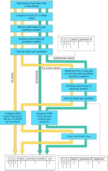
Figure 2: Flowchart of the workflows. The tables surrounded by broken lines show the minimum columns in the data frame at that point in the workflow.
For all workflows (Figure 2), the input point cloud is first con-verted into a Spark DataFrame, with each point represented as a row. A 62-bitZ-order index from the normalisedxandy coor-dinates is then assigned to each point. Its normalisation is based on the bounding box of the entire point cloud with (0,0) being the lower left corner and (231
−1,231
−1) being the upper right corner. From the index, the 2b-bit partition number (bbits per dimension) for each point is computed by bitwise shifting the in-dex to the right by (62−2b) bits. The dataset is then partitioned by the partition number then sorted by the index within each par-tition. The call to thepartition()method of the data frame would trigger a shuffle.
The first workflow,FLANN, selects theknearest neighbours (kNN) of each point by passing the contents of each partition to an ap-propriate third party library, which is Fast Library for Approx-imate Nearest Neighbors (FLANN)5in our implementation and experiments.
5
www.cs.ubc.ca/research/flann
The second workflow,WINDOW, exploits the windowing feature of the Spark DataFrames API. In this workflow, w preceding rows, wsucceeding rows and the current row, for a total of at most (2w+ 1) rows, are considered in each window. The dis-tance from each neighbouring point to the point is computed and thekpoints with the smallest distances are then selected as thek nearest neighbours. Neighbourhood-based computations, which may be through a third party library, can then be carried out fur-ther on this window.
Points near the partition boundaries may not have access to their true nearest neighbours which may be in other partitions. Par-titions can be made to span other parPar-titions by creating a mov-ing window buffer by replicatmov-ing the firstwand the lastwrows by as many partitions as needed. After partitioning and sorting with partitions, the result is a data frame of points which can then be treated as the input for FLANNor WINDOW. We call these modified workflows asFLANN-SPANandWINDOW-SPAN, respectively.
The spanning step is similar to the replication step in the kNN join algorithms discussed above. However, instead of adding a ran-dom vector, as in H-zKNNJ, or using a heuristic as in the method proposed by Lu et al. (Lu et al., 2012), we only base the partition-ing of the duplicates on the position of the row on the data frame sorted by the 62-bitZ-order.
Note that enabling spanning triggers a shuffle. To summarise,
FLANNandWINDOWrequire at least one shuffle whilstFLANN
-SPANandWINDOW-SPANrequire at least two shuffles. We expect that a workflow with spanning is slower than one without. With a handicap on runtime, we then have to investigate by how much accuracy improves with spanning, if it does, and what is the per-formance penalty for that improvement, assuming accuracy does improve.
3. EXPERIMENTAL RESULTS
We investigate the accuracyadefined as
a=nc
k, (1)
wherencis the number of correctly selected points andkis the
number of nearest neighbours, of the different workflows. We also look at the running time of the different workflows as various parameters of the point cloud and workflows vary.
We consider two kinds of synthetic point clouds: hemispherical and triangular wave. The former is a smooth point cloud while the latter is a sharper point cloud. The hemisphere is parameterized by its radiusrand is in the +zhalf-space. The triangular wave is parameterized by the number of peakspand is also in the +z half-space. The wave is travelling along thex-axis, that is,zis a function ofxonly.
The normals of both point clouds point upwards. Thus, the com-puted normals~ncin the workflow are reversed (−~nc) if they are
pointing upwards.
All experiments were implemented in Apache Spark 1.6.1 with a local master and 8 executor cores. The memory allocation is 8 GB for the driver and 1 GB for the executors. The workflows were implemented in Python.
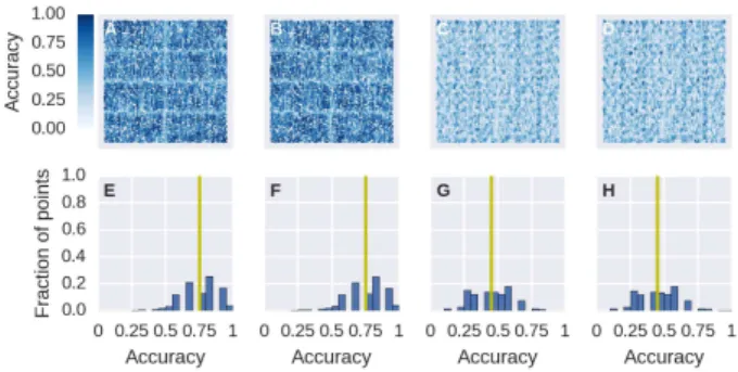
Figure 3: kNN accuracy in processing a hemispherical point cloud for a particular set of parameters for different workflows. In A-D, the points are projected onto thex-yplane. The colour corresponds to the kNN accuracy, defined as the fraction of cor-rectly selectedknearest neighbours, at each point. In E-H, the distribution of the accuracy is shown with the yellow vertical line indicating the value of the median. The workflows are: (A,E)
FLANN, (B,F)FLANN-SPAN, (C,G) WINDOW, (D,H) WINDOW
-SPAN. The values of the parameters are bit per dimensionb= 2, number of points per partitionNp= 1000, radiusr= 1, number
of nearest neighboursk = 20and look-back/look-ahead length w= 20.
3.1 Hemispherical Point Cloud
The hemispherical point cloud that we tested has a radiusr, cen-tred at the origin and is in the +zhalf-space. The motivation of selecting this geometry is to test the workflows on a smooth point cloud.
3.1.1 Spatial Accuracy Figure 3 shows the accuracy for hemi-spherical point clouds and workflows with bits per dimension b= 2, number of points per partitionNp = 1000, radiusr= 1,
k= 20, and window look-back/look-ahead lengthw= 20.
For this set of parameters, the results for the spanning and non-spanning versions ofFLANNandWINDOWare the same. Grid-like lines can be made out from Figures 3A and 3B and this is due to the lower accuracy of points near partition boundaries. Grid-like lines are also visible in Figures 3C and 3D but there are more lines and the spacing is much less, which suggests that the grid more likely due toZ-order indexing rather than due to partition boundaries.
The colours of Figures 3A and 3B are darker than those of Fig-ures 3C and 3D suggesting that the former are more accurate than the latter. There is a prominent peak ata= 0.9in Figures 3E and 3F corresponding to at least 50% of the points having an accuracy of at least 0.9. On the other hand, the distribution in Figures 3G and 3H are more spread and there is a less prominent peak at a= 0.65. Comparing the median of 0.9 forFLANNandFLANN
-SPANwith the median of 0.65 forWINDOWandWINDOW-SPAN, we conclude that FLANNand FLANN-SPAN are more accurate thanWINDOWandWINDOW-SPANat least for this set of param-eters. Furthermore,WINDOWandWINDOW-SPANhave a mini-mum accuracy of 0.05 i.e., only the point itself was selected as a nearest neighbour, which is less compared to a minimum accu-racy of 0.1 forFLANNand 0.2 forFLANN-WINDOW.
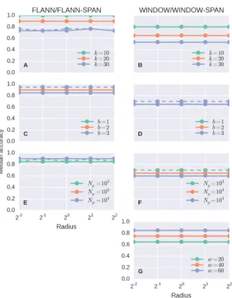
3.1.2 Effect of Different Parameters on Accuracy We now look at the accuracy of the workflows for different parameter val-ues as shown in Figure 4. Except for a few particular instances, the lines are constant with respect to the radius which suggests that accuracy does not depend on the curvature of the point cloud.
Figure 4: kNN accuracy in processing a hemispherical point cloud for different parameter values. Panels A, C and E em-ployed eitherFLANNorFLANN-SPANwhilst panels B, D E and G employed eitherWINDOWorWINDOW-SPAN. Solid lines cor-respond to FLANN or WINDOW whereas broken lines are for
FLANN-SPAN and WINDOW-SPAN. The varied parameters are (A-B) number of nearest neighboursk, (C-D) bits per dimen-sionb, (E-F) number of points per partitionNpand (F) window
look-back/look-ahead lengthw. If a parameter is not varying in a panel, value used isb= 2,Np= 1000,k= 20andw= 20.
Except for a few particular instances as well, the (broken) lines for the spanning version of each workflow coincide with the non-spanning version, which also suggests that the added complica-tion of spanning does not usually result to any significant im-provement in the accuracy.
One can easily notice in Figure 4A that the median accuracy for k = 10 is 1.0 which implies that as long ask ≤ 10then the selected nearest neighbours are likely to be all correct. Ask in-creases the accuracy dein-creases, which is expected since as more neighbours are required, the likelihood of one of these neighbours being outside the partition increases. Adding spanning mitigated this partition effect slightly as shown in Figure 4A but the line fork = 30(FLANN-SPAN) is too close and too intertwined (the accuracy atr = 2is worse than forFLANN) for us to make any stronger conclusions. The drop in the accuracy due to increasing k > kthresafter some thresholdkthresseems to be nonlinear since
the change in median accuracy fromk = 10tok = 20is 0.1 whilst fromk= 20tok= 30is 0.17.
Comparing the results with that forWINDOWandWINDOW-SPAN
(Figure 4B), the difference in the accuracy is more apparent. Whilst fork = 10, the median accuracy forFLANNandFLANN-SPAN
kincreases but unlike inFLANNandFLANN-SPAN, the change is more linear with a drop of 0.15 fromk= 10tok= 20, and 0.12 fromk= 20tok= 30.
A smallerbmeans more points per partition for a constant total number of pointsNin the point cloud. However, theNpis held
constant so what we are observing in Figures 4C and 4D are the effect of theZ-order and partitioning on the accuracy. In Fig-ure 4C, the median precision forFLANN is 0.9 forb = 1and b= 2and 0.85 forb= 3. The values are the same forb= 1and b= 2forFLANN-SPANbut jumps to0.95forb= 3. It seems that forb= 3, the partitions are too small that a significant number of nearest neighbours are in other partitions such that enabling spanning significantly improves and beats the median precision for smaller values ofb.
The advantage of enabling spanning is also observed in Figure 4D albeit the best median precision of 0.7 is still less than the worse precision of 0.85 forFLANN. These results suggest that spanning can improve accuracy for some minimum value ofb although we cannot confidently state the value of that threshold at this point. These also support the possible use of spanning in working around issues related to partitioning.
WhenNpis increased, the number of points near a partition
bound-ary increases but so are the number of points that are inside and that have all their nearest neighbours within the partition. The rate of increase of the latter should be more than that of the for-mer so the net effect would be that the accuracy tends to increase asNp increases. This effect is somewhat observed in Figure 4E
where the median accuracy for FLANN jumped from 0.85 for Np = 10
2
to 0.9 forNp = 10
3
and stayed there forNp = 10
4 . Spanning improved the median accuracy ofFLANN-SPANto 0.9 forr= 2−2
andr= 22
, which may be related to the area cov-ered by the point cloud in corner partitions.
The expected effect of Np is opposite to what is observed in
Figure 4F. The median accuracy of WINDOW is 0.65 for both Np = 10
2
andNp = 10
3
but drops to 0.6 forNp = 10
4 . This unexpected result can be explained by recalling thatWINDOW re-lies on sorting based onZ-order. As more points are added, the bias against nearest neighbours that are not along the traversal direction of theZ-order increases leading to a decrease in the accuracy. Enabling spanning improves the median accuracy to Np= 0.7.
Not surprisingly, increasingw improves accuracy as shown in Figure 4G. In this case, the median accuracy linearly increased from 0.65 forw = 20to 0.85 forw = 60. SinceNp = 1000,
this corresponds to a window size of 4.1% to 12.1% of the number of points in the partition. Spanning has no effect on the median accuracy.
3.2 Triangular Wave Point Cloud
We test the workflows on a non-smooth, triangular wave point cloud withppeaks parallel to they-axis and residing in the +z half-space.
3.2.1 Spatial Accuracy The accuracy distribution ofFLANN
andFLANN-SPAN, andWINDOWandWINDOW-SPAN(Figure 5) for a triangular wave point cloud is similar within each pair. The triangular wave peaks are oriented vertically in the figure.
There are noticeable horizontal lines in Figures 5A and 5B, which are due to the lower accuracy of points near partition boundaries. There is only one visible vertical line and this corresponds to the
Figure 5: kNN accuracy in processing a triangular wave point cloud for a particular set of parameters for different workflows. In A-D, the points are projected onto thex-yplane. The colour cor-responds to the kNN accuracy, defined as the fraction of correctly selectedknearest neighbours, at each point. In E-H, the distribu-tion of the accuracy is shown with the yellow vertical line indi-cating the value of the median. The workflows are: (A,E)FLANN, (B,F)FLANN-SPAN, (C,G)WINDOW, (D,H)WINDOW-SPAN. The values of the parameters are bit per dimensionb= 2, number of points per partitionNp= 1000, number of peaksp= 3, number
of nearest neighboursk = 20and look-back/look-ahead length w= 20.
only triangular wave peak that coincides with a partition bound-ary. Taken together, the position of the visible lines imply that points near partition boundaries are not guaranteed to have lower accuracy than inner points.
It is harder to identify any prominent features in Figures 5C and 5D but, upon closer inspection, a light vertical line can be made out at the middle, which again corresponds to the triangular wave peak that coincides with a partition boundary. Two dark lines at each side of the light vertical line can also be seen and these correspond to triangular wave peaks and troughs.
All workflows have lesser accuracy (Figure 5E-H) when the input is a triangular wave point cloud instead of a hemispherical point cloud. From a median accuracy of 0.9 for a hemispherical point cloud, the median accuracy ofFLANNandFLANN-SPANfor a tri-angular wave point cloud is 0.75. Similarly, the median accuracy ofWINDOWandWINDOW-SPANdropped from 0.65 to 0.45. The peaks are less prominent and shifted to the left as well. The dip in the accuracy is expected because a nearest neighbour of a point may be on the other side of a peak or dip and this would be farther along in sequence of theZ-order.
3.2.2 Effect of Different Parameters on Accuracy There is a general trend of decreasing accuracy for increasing peaks (Fig-ure 6), which is expected.FLANNandFLANN-SPANare also more accurate thanWINDOWandWINDOW-SPAN.
Unlike with hemispherical point cloud wherek≤10results to a median accuracy of 1.0 forFLANNandFLANN-SPANin all values ofrconsidered, for triangular wave point clouds (Figure 6A), it is 1.0 only ifp≤2. This can be extended top= 3if spanning is enabled but ifp > 3, the median accuracy is constant at 0.9. Enabling spanning also improves the median accuracy forp = 3when k = 20. However, spanning results in lower median precision fork= 30. Spanning has no effect on the accuracy of
WINDOWandWINDOW-SPAN(Figure 6B).
Figure 6: kNN accuracy in processing a triangular wave point cloud for different parameter values. Panels A, C and E em-ployed eitherFLANNorFLANN-SPANwhilst panels B, D E and G employed eitherWINDOWorWINDOW-SPAN. Solid lines cor-respond to FLANN or WINDOW whereas broken lines are for
FLANN-SPANand WINDOW-SPAN. The varied parameters are (A-B) number of nearest neighboursk, (C-D) bits per dimen-sionb, (E-F) number of points per partitionNp and (F) window
look-back/look-ahead lengthw. If a parameter is not varying in a panel, value used isb= 2,Np = 1000,k= 20andw= 20.
more sensitive betweenk= 10andk= 20than betweenk= 20 andk= 30.
The curves in Figure 6C are overlapping so it is difficult to ascer-tain the effect ofbon the median accuracy. However,b= 3tends to have the smallest median accuracy for FLANNbut enabling spanning makes the workflow the most accurate among the curves in Figures 6C and D. This is more acutely seen in Figure 6D wherein the curve forb = 3(WINDOW-SPAN) is clearly above the other curves, which are coinciding. The same behaviour of b = 3(WINDOW-SPAN) is also seen for a hemispherical point cloud and the same explanation holds.
The curves are overlapping in Figures 6E and F so it is difficult to issue a strong statement on the effect ofNpon the median
ac-curacy of different workflows. The observation on hemispherical point clouds that median accuracy tends to increase withNpfor
FLANNandFLANN-SPANbut tends to decrease forWINDOWand
WINDOW-SPANno longer holds.
There is a general trend of increasing median accuracy for in-creasingw as shown in Figure 6G. However, the trend is less defined than in hemispherical point cloud because of overlapping curves. There is an improvement in the median accuracy in some instances if spanning is enabled.
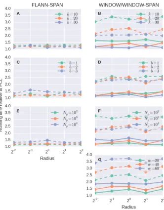
Figure 7: Relative running times of kNN for processing a hemi-spherical point cloud. Relative running time is computed as the ratio between the running time of each workflow and the running time ofFLANNand is based on the mean of five trials. Panels A, C and E are forFLANN-SPANonly whilst panels B, D E and G employed eitherWINDOWorWINDOW-SPAN. Solid lines cor-respond toWINDOWwhereas broken lines are forFLANN-SPAN
andWINDOW-SPAN. The varied parameters are (A-B) number of nearest neighboursk, (C-D) bits per dimensionb, (E-F) number of points per partitionNpand (F) window look-back/look-ahead
lengthw. If a parameter is not varying in a panel, the value used isb= 2,Np= 1000,k= 20andw= 20.
3.3 Running Time
The running time for both hemispherical and triangular wave point clouds are similar so we only analyse that of the hemispherical point cloud.
The fastest workflow isFLANNas shown in Figure 7 where all relative running times are greater than 1.0. Spanning workflows are also slower than their corresponding non-spanning workflows because these involve an extra shuffle.
The relative running times ofFLANN-SPANwith respect tor (Fig-ure 7A) is almost constant for k = 10andk = 20with the former having consistently larger relative running times (1.29 to 1.32) than the latter (1.20 to 1.25). The relative running time for k= 30is more erratic with it being almost the same as ink= 10 forr= 2−1
and as ink= 20forr= 21
. The apparent decreas-ing relative runndecreas-ing time askincreases suggest that the overhead of spanning decreases askincreases.
The somewhat erratic behaviour of the relative running time asr increases is also observed (Figure 7B) inWINDOWandWINDOW
the relative running time ofWINDOWdoes not exceed 1.7 com-pared to that ofWINDOW-SPANwhich is at least 2.0. In general, the relative running time ofWINDOW-SPANis about twice that of
WINDOW.
The relationship between relative running time andrremains in-definite whenb(Figure 7C) is varied. The effect ofbitself is also irregular with the line forb= 1criss-crossing the line forb= 2. However, the line forb= 3which is not too surprising because largerbimplies more partitions to shuffle.
Enabling spanning onWINDOW(Figure 7D) would result to an around 75% increase in relative running time for varyingb. The lines for differentbare too intertwined to conclude as to the effect ofron the relative running time.
There is an unexplained dip atr = 21
that can be seen in Fig-ure 7E-G. The maximum relative running time is atr = 20
as well. Although there is a superlinear increase in the relative run-ning time (Figure 7E) asNp is increased, the maximum relative
running time remains below 1.5. Enabling spanning onWINDOW
(Figure 7F) doubles the relative running time and can exceed three times the running time ofFLANNforNp = 10
4
. Increas-ingw(Figure 7G) results to a larger relative running time and enabling spanning doubles running time.
4. CONCLUSION
The increasing volume of point clouds increases the need for pro-cessing them in parallel. This would require breaking them down into partitions and distributing across multiple machines. Data locality is important here, which is the concept that data must be on the processing machine as much as possible because network transfer would be very slow.
We proposed a Z-order-based partitioning scheme and imple-mented it on Apache Spark. We showed that it is an effective method and a convenient one as well because third-party libraries and code may still be used. Enabling spanning may not be too useful as well as the improvement in median accuracy is mini-mal.
We have only investigated the accuracy of kNN selection but the accuracy of other nearest-neighbourhood-based operations may be investigated as well. For example, extracting normals from point clouds using PCA may prove to be more robust to the ef-fects of partitioning.
An advantage ofZ-order partitioning is that the level of detail i.e., partition size, can be easily adjusted. We intend to imple-ment an adaptiveZ-order indexing such that partitions can be automatically adjusted to have a more constant number of points per partition.
ACKNOWLEDGEMENTS
We would like to acknowledge that this work is in part supported by EU grant FP7-ICT-2011-318787 (IQmulus).
REFERENCES
Connor, M. and Kumar, P., 2010. Fast construction of k-nearest neighbor graphs for point clouds. IEEE Transactions on Visual-ization and Computer Graphics 16(4), pp. 599–608.
Eldawy, A., Alarabi, L. and Mokbel, M. F., 2015. Spatial Par-titioning Techniques in SpatialHadoop. Proc. VLDB Endow. 8(12), pp. 1602–1605.
Lawder, J. K. and King, P. J. H., 2000. Using Space-Filling Curves for Multi-dimensional Indexing. In: B. Lings and K. Jef-fery (eds), Advances in Databases, Lecture Notes in Computer Science, Springer Berlin Heidelberg, pp. 20–35.
Lu, W., Shen, Y., Chen, S. and Ooi, B. C., 2012. Efficient Pro-cessing of K Nearest Neighbor Joins Using MapReduce. Proc. VLDB Endow. 5(10), pp. 1016–1027.
Nishimura, S., Das, S., Agrawal, D. and Abbadi, A. E., 2012. MD-HBase: design and implementation of an elastic data infras-tructure for cloud-scale location services. Distributed and Parallel Databases 31(2), pp. 289–319.
Orenstein, J. A. and Manola, F. A., 1988. PROBE spatial data modeling and query processing in an image database application. IEEE Transactions on Software Engineering 14(5), pp. 611–629.
Swart, L. T., 2010. How the Up-to-date Height Model of the Netherlands (AHN) became a massive point data cloud. NCG KNAW.
Wei, L.-Y., Hsu, Y.-T., Peng, W.-C. and Lee, W.-C., 2014. In-dexing spatial data in cloud data managements. Pervasive and Mobile Computing 15, pp. 48–61.
You, S., Zhang, J. and Gruenwald, L., 2015. Large-scale spatial join query processing in Cloud. In: 2015 31st IEEE International Conference on Data Engineering Workshops (ICDEW), pp. 34– 41.