M and X Class Flares During 2011 to 2013 and their Connection to Auroral Electrojet Indices

(1)

M and X Class Flares During 2011 to 2013 and their

Connection to Auroral Electrojet Indices

Debojyoti Halder

Department of Physics, University of Kalyani, Kalyani 741235, West Bengal, India

Email: debojyoti829@gmail.com

Abstract− Solar bursts recorded in the frequency range 50 to 300 MHz by using log periodic dipole array over Kalyani (22°58´N, 88°46´E) have been statistically analyzed for the years 2011-2013. Scatter plots of flare intensity for both M- and X-class flares as well as the number of occurrences of the two categories have been examined. The characteristics of the auroral electrojet indices are correlated directly to the solar flare activity. The auroral indices data obtained from various sources are sorted accordingly. The daily averaged data of the auroral indices are plotted for a period of 5 years, 2009 to 2013. Regression analysis of the indices data has been done meticulously. The regression analysis data are also plotted as residual plots and line fit plots. We have tried to discuss the possible connection between the occurrences of solar flares and the auroral electrojet indices.

Keywords – Solar Flare, M- and X-Class Flare, Auroral Electrojet (AE) Index, Regression Analysis, Solar Radio Emission.

I. I

NTRODUCTION

A solar flare is a sudden flash of brightness observed over the Sun's surface, interpreted as release of huge amount of energy. They are habituallytrailed by a massive coronal mass ejection (CME)[1]. The flares eject clouds of electrons, ions, and atoms through the corona of the sun into space. Solar flares affect all layers of the solar atmosphere, when the plasma medium is heated. They produce radiation across the electromagnetic spectrum at all wavelengths. Flares occur in active regions around sunspots, where intense magnetic fields penetrate the photosphere to link the corona to the solar interior [2]. During the study of radio signals originating from Sun, solar flares can be prominently recorded. X-class flares are the biggest and strongest of all the solar flares. M-class flares are the medium large flares. They cause small to moderate radio blackouts on the daylight side of the Earth. Small radiation storms can also happen occasionally [3]. Only strong M-class flares which are long in duration and are accompanied by an Earth-directed Coronal Mass Ejection (CME) could cause auroral storming on the middle latitudes.

The Auroral Electrojet Index (AE) is designed to provide a global, quantitative measure of auroral zone magnetic activity produced by enhanced ionospheric currents flowing below and within the auroral oval. Ideally, It is the total range of deviation at an instant of time from quiet day values of the horizontal magnetic field around the auroral oval. Horizontal magnetic component recordings from a set of globe-encircling stations are plotted to the same time and amplitude scales relative to their quiet-time levels and then graphically superposed.

The upper and lower envelopes of this superposition define the AU (amplitude upper) and the AL (amplitude lower) indices, respectively. The difference between the two envelopes determines the AE (Auroral Electrojet) index, i.e., AE = AU - AL. AO is defined as the average value of AU and AL [4]. Defined and developed by Davis and Sugiurain 1966, AE has been usefully employed both qualitatively and quantitatively as a correlative index in studies of sub-storm morphology, the behavior of communication satellites, radio propagation, radio scintillation, and the coupling between the interplanetary magnetic field and the earth's magnetosphere. For these varied uses, AE possesses advantages over other geomagnetic indices such as, it can be derived on an instantaneous basis or from averages of variations computed over any selected interval; it is a quantitative index which, in general, is directly related to the processes producing the observed magnetic variations; its method of derivation is relatively simple, digital, and objective and is well suited to present computer processing techniques; and it may be used to study either individual events of statistical aggregates [4].Some interesting results of statistical analyse from our received data related to M- and X-class solar flares as observed during 2011 to 2013 using log periodic dipole array (LPDA) over Kalyani (220 58/ N, 880 28/ E), West Bengal are reported in this paper. Those results are one way or another connected to the auroral electrojet indices. The four auroral indices AE, AU, AL and AO are plotted with the calendar dates of years 2010 to 2013. The data are then processed statistically through regression analysis and plotted as residual and line fit plots. The connection between the M and X-class flares and the auroral electrojet indices are critically examined in this paper.

II. M-

AND

X-C

LASS

F

LARES

Solar flares are usually classified in two ways. One class is by differentiating flares by theirX-ray intensity and other is by their H-alpha spectra. The X-ray intensity classification is as table I follows. Solar flares are classified as A, B, C, M, X and recently Z according to their peak flux (in W/m2) of 100 to 800 picometre X-rays near Earth, as measured on the GOES spacecraft.

Table I: Classification of solar flare by X-ray intensity [5] Classification Peak Flux Range at 100-800 pm

(W/m2)

A < 10−7

B 10−7 - 10−6

C 10−6 - 10−5

(2)

X 10−4 - 10−3

Z > 10−3

Each category has nine subdivisions ranging from 1 to 9; e.g. C1 to C9, M1 to M9 etc. A multiplier is used to indicate the level within each class, e.g., M 6 = 6 X 10

-5

W/m2. However, the extreme event in 1859 is theorized to have been well over X40 so a Z class designation is possible [6].

The second classification is H-alpha classification which is an earlier flare classification based on Hα spectral observations given in table II. The scheme uses both the intensity and emitting surface. The classification in intensity is qualitative, referring to the flares as: Faint (f), Normal (n) or Brilliant (b). The emitting surface is measured in terms of millionths of the hemisphere and is described below. A flare then is classified taking S or a number that represents its size and a letter that represents its peak intensity, e.g.: Sn is a normal sub-flare.

Table II: Classification of solar flare by Hα spectral observations (The total hemisphere area AH = 6.2 × 1012

km2) [5]

Classification Corrected area [millionths of hemisphere]

S < 100

1 100 - 250

2 250 - 600

3 600 - 1200

4 > 1200

We have recorded the solar flares in our laboratory in Kalyani using log periodic dipole array (LPDA) operating between 50 to 300 MHz.Table III comprises the occurrences of flares as recorded in our receiving system during 2011 to 2013 under the two categories M and X as defined above.

Table III: List of M and X-Class Solar Flares during 2011-2013 Showing Responses in Radio Signals Year M-Class X-Class Total no. of flares

2011 88 6 94

2012 62 4 66

2013 84 11 95

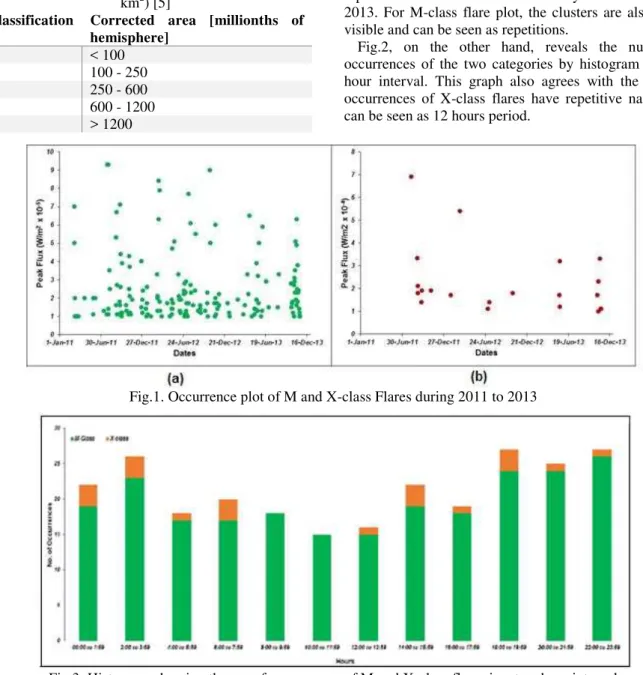
Fig.1 shows a scatter plot of flare intensity with the corresponding dates of occurrences for both M- and X-class. Fig.1(a) and 1(b) respectively shows plotted scattered data for the M-class and X-class respectively. We can clearly see from fig. 1 that either M-class or X-class flares has a tendency to form cluster. As for X-X-class flare intensity plot, we can say that they follows almost repetition after 6 months from January 2011 to December 2013. For M-class flare plot, the clusters are also clearly visible and can be seen as repetitions.

Fig.2, on the other hand, reveals the number of occurrences of the two categories by histogram in a two hour interval. This graph also agrees with the fact that occurrences of X-class flares have repetitive nature here can be seen as 12 hours period.

Fig.1. Occurrence plot of M and X-class Flares during 2011 to 2013

(3)

III. A

URORAL

E

LECTROJET

I

NDICES

D

ATA

A

NALYSES

AE indices were determined first at the Geophysical Institute of the University of Alaska, then at the Goddard Space Flight Center in Greenbelt and then at the World Data Center and recently at the World Data Center C2 for Geomagnetism in Kyoto with assistance from the National

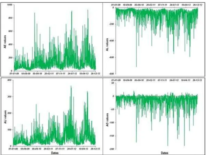
Institute of Polar Research in Tokyo [4]. Here in fig. 3, we plotted the daily averaged data of four auroral indices in a time duration of 5 years 2009 to 2013. For each index, there is a repetitive nature of graph for every years clearly evident from fig. 3. Maximum of each index is clustered around a four-month period May to August for each year 2009 to 2013. The values of every index are increasing as the years passing by but the trend is same.

Fig.3. Plots of allthe four auroral index for the years 2009-2013

The trend line equations for the four plots presented in table IV showing values of slopes, intercepts and R-squared values for the four cycles. The table reveals that for AE, AU and Al the plots are of nearly same trend but for AO index is abruptly different.

Table IV: some parameters derived from above four plots

Indices m C R2

AE 0.0566 - 2175.8 0.0602

AU 0.0231 - 888 0.0699

AL - 0.0336 + 1287.6 0.0507

AO - 0.0054 + 203.72 0.0186

IV. R

EGRESSION

A

NALYSIS

In modern science, regression analysis is a necessary part of virtually almost any data reduction process. In a regression analysis we study the relationship, called the regression function, between one variable y, called the dependent variable, and several others xi, called the

independent variables. Regression function also involves a set of unknown parameters bi. If a regression function is linear in the parameters, we term it a linear regression model. Linear regression models with more than one independent variable are referred to as multiple linear models, as opposed to simple linear models with one independent variable. A residual (or fitting error), on the other hand, is an observable estimate of the unobservable statistical error. The sum of the residuals within a random sample is necessarily zero, and thus the residuals are necessarily not independent. If we assume a normally distributed population with mean μ and standard deviation σ, and choose individuals independently, then we have,

X1, … ,Xn~ N (μ, σ2)

and the sample mean,

� =�1+⋯+��

is a random variable distributed thus:

(4)

�� = �� − �

In regression analysis, the distinction between errors and residuals is subtle and important. Given an unobservable function that relates the independent variable to the dependent variable the deviations of the dependent variable observations from this function are the unobservable errors. If one runs a regression on some data,

then the deviations of the dependent variable observations from the fitted function are the residuals.

A. Regression Analysis of AE, AU, AL and AO

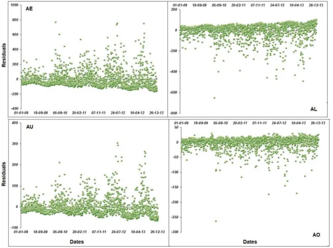
Fig. 4 depicts the plots of residuals of the regression analysis of the four auroral electrojet indices values for the 5 years period we have taken. It shows that the variations for residuals in any year are monotonically increasing than previous years.

Fig.4. Residual plots of all theindices

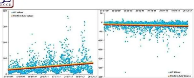
Fig. 5 shows the four line fit plots of regression analysis for the same indices for the same period. Here we have plotted the four auroral indices and its best fit graph with

(5)

Table V summarizes the parameters of the regression analysis of the four auroral indices. It can be well noticed from table V that all the parameters „Multiple R‟, „R2‟,

„Adjusted R2‟ and Standard error‟ are nearly same for the

three indices AE, AU and AL but for AO they are surprisingly different.

Table V. Regression Statistics for Auroral Electrojet indices

Indices Multiple R R Square Adjusted R Square Standard Error

AE 0.245421475 0.060231701 0.059716477 117.9966677

AU 0.26435431 0.069883201 0.069373269 44.36192136

AL 0.225059167 0.050651629 0.050131153 76.6679383

AO 0.130633339 0.017065069 0.016526179 21.08806356

V. C

ONCLUSION

A solar flare is an explosion on the sun which happens when energy stored in twisted magnetic fields is suddenly released. Flares produce a burst of radiation across the electromagnetic spectrum with many forms - electro-magnetic (gamma rays and x-rays), energetic particles (protons and electrons) and mass flows. The biggest flares are categorized as x-class flares which exhibit greater value of voltage than m-class flare. The connection between occurrences of the solar flares and the increase and decrease in values of auroral electrojet indices is definite and is strongly supported by our data plots of indices. On those dates strong solar flares have been occurred the values of the auroral indices had a sudden increase. We can see that there are no x-class flares occurred in 2009 and 2010. The plots of ae to ao indices shows that the magnetic activity of the sun was much lower in those two years. So it can be concluded that if there is a solar flare or any associated solar events, there is increase in value of auroral electrojet indices and accordingly in magnetic activity of the sun.

A

CKNOWLEDGEMENT

Author is thankful to the CSIR for awarding him a Net fellowship.

R

EFERENCES

[1] G.Kopp, G. Lawrence and G. Rottman, (2005). "The Total

Irradiance Monitor (TIM): Science Results". Solar Physics, 20 (1–2) 129–139.

[2] D. H. Menzel, F. L. Whipple, G. De Vaucouleurs, "Survey of the

Universe", Pearson Education Limited,1970.

[3] Grubor, D., Sulic, D. and Zigman, V. (2005) “Influence of Solar

X-ray flares on the earth-ionosphere waveguide”, Serb. Astron.,

Vol. 171, 29-35.

[4] T. N. Davis and M. Sugiura, (1966), “Auroral electrojet activity

index AE and its universal time variations”, Journal of

Geophysical Research, Vol71, Issue 3,p 785–801,

[5] E. Tandberg-Hanssenand A. G. Emslie, (1988). Cambridge

University Press, ed. "The physics of solar flares".

[6] http://science.nasa.gov/science-news

A

UTHOR

’

S

P

ROFILE

M and X Class Flares During 2011 to 2013 and their Connection to Auroral Electrojet Indices