www.atmos-chem-phys.net/15/8739/2015/ doi:10.5194/acp-15-8739-2015
© Author(s) 2015. CC Attribution 3.0 License.
Contrail life cycle and properties from 1 year of MSG/SEVIRI
rapid-scan images
M. Vázquez-Navarro1, H. Mannstein1,†, and S. Kox1,*
1Deutsches Zentrum für Luft- und Raumfahrt, Institut für Physik der Atmosphäre, Oberpfaffenhofen, Germany *now at: European Organisation for the Exploitation of Meteorological Satellites (EUMETSAT), Darmstadt, Germany †deceased
Correspondence to:M. Vázquez-Navarro ([email protected])
Received: 26 September 2014 – Published in Atmos. Chem. Phys. Discuss.: 10 March 2015 Revised: 18 May 2015 – Accepted: 10 June 2015 – Published: 10 August 2015
Abstract.The automatic contrail tracking algorithm (ACTA) – developed to automatically follow contrails as they age, drift and spread – enables the study of a large number of contrails and the evolution of contrail properties with time. In this paper we present a year’s worth of tracked contrails, from August 2008 to July 2009 in order to derive statisti-cally significant mean values. The tracking is performed us-ing the 5 min rapid-scan mode of the Spinnus-ing Enhanced Visible and Infrared Imager (SEVIRI) on board the Me-teosat Second Generation (MSG) satellites. The detection is based on the high spatial resolution of the images provided by the Moderate Resolution Imaging Spectroradiometer on board the Terra satellite (Terra/MODIS), where a contrail detection algorithm (CDA) is applied. The results show the satellite-derived average lifetimes of contrails and contrail-cirrus along with the probability density function (PDF) of other geometric characteristics such as mean coverage, distri-bution and width. In combination with specifically developed algorithms (RRUMS; Rapid Retrieval of Upwelling irradi-ance from MSG/SEVIRI and COCS (Cirrus Optical proper-ties derived from CALIOP and SEVIRI), explained below) it is possible to derive the radiative forcing (RF), energy forc-ing (EF), optical thickness (τ) and altitude of the tracked con-trails. Mean values here retrieved are duration, 1 h; length, 130 km; width, 8 km; altitude, 11.7 km; optical thickness, 0.34. Radiative forcing and energy forcing are shown for land/water backgrounds in day/night situations.
1 Introduction
One of the least understood influences that the air traffic has in the atmosphere results from contrail formation. When the conditions suitable for contrail formation occur, contrails form and spread, therefore increasing the cloud cover (Schu-mann et al., 2012a). In order to better understand the radiative forcing of contrails and aviation-induced cirrus clouds, it is necessary to thoroughly study their onset, development and the evolution of their physical properties. Despite the atten-tion and numerous studies on radiative forcing (RF) and other properties of contrail and contrail cirrus in the past decades (Bakan et al., 1994; Mannstein et al., 1999; Minnis et al., 2004; Palikonda et al., 2005; Atlas et al., 2006; Meyer et al., 2007; Burkhardt and Kaercher, 2011; Iwabuchi et al., 2012; Duda et al., 2013, etc.), the level of scientific understanding of this particular aspect of aviation is still classified as low, and that of induced contrail cirrus as very low (Lee et al., 2009). The current contrail RF estimates are 0.05 W m−2
(including contrail cirrus), with large uncertainties (Stocker et al., 2013). Although this global value may seem small, the local effect is larger in regions with high contrail cov-erage. The difficulty in distinguishing natural cirrus clouds from aviation-induced cirrus clouds is one of the roots of the problem (Mannstein and Schumann, 2005).
Figure 1.Area covered by the MSG/SEVIRI Rapid Scan Service.
other properties. The mean optical depths of the contrail cir-rus under study ranged from 0.32 to 0.43. They also observed that these values were 2–3 times larger than the correspond-ing values for the adjacent linear contrails. Not many studies have focused on the observation of contrail-to-contrail-cirrus evolution because, in the absence of a proper tracking tech-nique, the analysis is limited to case studies. Combinations of satellite information and ground-based lidar measurements, such as in the Atlas et al. (2006) case study, show a lifetime of more than 2 h and a mean optical thickness of 0.35. Duda et al. (2004) studied the development of contrail clusters over the Great Lakes and derived τ from 0.1 to 0.6 for contrails that lasted several hours. Graf et al. (2012) studied the cirrus cover cycle and observed timescales between 2.3 to 4.1 h for contrail cirrus and 1.4 to 2.4 h for linear contrails.
Satellite imagery provides an excellent tool for observ-ing contrail development. On one hand, polar orbitobserv-ing satel-lites have the advantage of a good spatial resolution, which is useful for locating linear contrail structures. On the other hand, geostationary satellites have the capability of observ-ing events that vary in very short timescales. Therefore, a combination of the temporal resolution of geostationary satellites and the spatial resolution of polar orbiting satel-lites is essential in the study of quick cloud processes. In this paper we have used Terra/MODIS images for the contrail lo-cation. It is a polar orbiting instrument with a 1×1 km nadir
resolution. For the tracking and the retrieval of the physical properties we used MSG/SEVIRI (Spinning Enhanced Vis-ible and Infrared Imager (SEVIRI) on board the Meteosat Second Generation (MSG)) (Schmetz et al., 2002), a geosta-tionary instrument with a 3 km×3 km nadir resolution. The
Rapid Scan Service (RSS) provides MSG/SEVIRI images of the upper third of the MSG disk with a temporal resolution of 5 min; this short time step between two consecutive images makes possible the identification and tracking of single con-trail events. The area scanned in the RSS mode is shown in Fig. 1. It covers heavily flown areas such as Europe and part of the North Atlantic Ocean.
In this paper, two main algorithms are used to locate and track the development of contrails: a contrail detection algo-rithm (CDA) is used for the location (Mannstein et al., 1999) and an automatic contrail tracking algorithm (ACTA) is used for contrail tracking (Vázquez-Navarro et al., 2010). CDA
is based on the fact that contrails are ice clouds that have a linear structure when they form. It has already been used to study linear contrail coverage on several regions of the Earth: central Europe (Meyer et al., 2002), North America (Palikonda et al., 2005), eastern North Pacific (Minnis et al., 2005), southern and eastern Asia (Meyer et al., 2007) and the North Atlantic (Graf et al., 2012). A modified version of the algorithm has recently been used by Duda et al. (2013); Bedka et al. (2013) and Spangenberg et al. (2013) to estimate several linear contrail properties in the Northern Hemisphere. When they are past the linear stage, contrails spread and lose their distinct shape and the CDA can no longer detect them. At first sight, these aged contrails are indistinguish-able from natural cirrus clouds, but it is possible to continue tracking them by combining the information on location and displacement when such data are available. The ACTA tracks these linear contrails in a similar way as a human observer does. It considers that contrails in consecutive images re-tain most of their shape while only changing slightly, and uses this information to identify a given contrail through-out its lifetime. The combined use of CDA on Terra/MODIS and ACTA on MSG/SEVIRI(RSS) provides information on the lifespan of contrails and also on distribution, width and length. The next section describes the exact settings of the CDA used as well as a thorough description of the combina-tion of ACTA and CDA.
Two recently developed algorithms to derive cloud prop-erties are additionally used in this paper to retrieve contrail radiative forcing, energy forcing, optical thickness and cloud top height: RRUMS (Rapid Retrieval of Upwelling irradi-ance from MSG/SEVIRI, Vázquez-Navarro et al., 2013) and COCS (Cirrus Optical properties derived from CALIOP and SEVIRI, Kox et al., 2014). The RRUMS algorithm measures outgoing top-of-atmosphere (TOA) reflected solar radiation (RSR) and outgoing long-wave radiation (OLR) using SE-VIRI channels. The forcing can be derived from this infor-mation using a background assumption explained below. The COCS algorithm retrieves optical thickness and top altitude of cirrus clouds through a combination of SEVIRI infrared channels. Both algorithms are described in detail below.
The following sections explain in detail the algorithms used for the production of the data set and the retrieval of the contrail properties. This is followed by an analysis of the obtained results. Note that throughout this paper, the word contrail refers both to linear contrail and contrail cirrus.
2 Algorithms and data description 2.1 CDA and ACTA
Radiometer carried on NOAA satellites (NOAA/AVHRR). It is based both on the brightness temperature difference, BTD, between the 10.8 and 12 µm channels and on the 12 µm brightness temperature. Ice crystals present differ-ent behaviours in those two wavelengths while other atmo-spheric and surface properties are similar for both channels (Lee, 1989). Images are processed and normalised, and the resulting scenes are screened for linear contrails using a fil-ter with a kernel size of 19×19 pixels in several directions
to include all possible orientations of the contrails. Finally, the features fulfilling a given set of geometrical and physical thresholds are identified and labelled as linear contrails. The resulting linear contrails will then be used as input for the tracking algorithm.
To create a database with the highest number of auto-matically tracked contrails and the least possible human in-tervention, it was necessary to adapt the CDA to produce the lowest false alarm rate possible. This decision has lead inevitably to a lower detection efficiency. The geometrical thresholds used in CDA for this work are a minimum length threshold (47 MODIS pixels), a minimum number of pix-els threshold (19 pixpix-els) and an alignment threshold (cor-relation coefficient >0.975). Threshold lengths larger than the minimum-number-of-pixels threshold allow the contrail to be a non-connected structure. The physical thresholds are scene-dependent and are related to the sum of the normalised images, the brightness temperature difference and the gradi-ent of the temperature in channel 12 µm. The output of CDA is a list with the geographical position ofNlinear contrails.
Having located theN MODIS linear contrails, we mapped them on the SEVIRI grid. A constant height of 10 km for each contrail was considered for the parallax correction. Then, ACTA (Vázquez-Navarro et al., 2010) was applied to the aforementioned contrails. ACTA is based exclusively on the BTD between SEVIRI infrared channels 10.8 and 12.0 µm. Based on the position of the starting contrailCi at
timet=t0, ACTA looks for the same contrailCi in the
fol-lowing SEVIRI image, at timet+1t:Ci(t+1t ). If found,
ACTA uses the information about the new position to con-tinue iterating, now usingt+1t as initial time. When the contrail Ci cannot be tracked any longer, ACTA returns to t0and repeats the process backwards in time (t−1t). When
the backwards tracking is completed, ACTA proceeds to the next contrail on the input list. This procedure allows the de-termination of the contrail lifetime, n1t+n′1t, from its first occurrence in SEVIRI at timet0−n1t until it can no
longer be discriminated from its surroundings by the satel-lite att0+n′1t, regardless of the MODIS overpass timet0
(see schematic representation of ACTA in Fig. 2). Tracking takes place while there is a contrast between contrail and background in the BTD image. A lack of contrast causes the tracking to stop. This could be due to contrails thinning out becoming indistinguishable, evolution of a cluster containing a group of contrails into a widespread homogeneous cirrus cloud, contrails drifting under pre-existing cirrus cloud, etc.
Figure 2.Schematic representation of ACTA. Input: list of linear
contrails detected by the CDA on MODIS (Vázquez-Navarro et al., 2010).
Some of the contrails are sufficiently resolved for MODIS (nadir resolution 1×1 km) but not enough for SEVIRI (nadir resolution 3×3 km). This causes some of the input contrail scenes in SEVIRI to be empty. Further problems such as wrong identification of contrails by the CDA, for instance, coastlines or linear-shaped cloud streaks, were also present. Despite tuning the CDA to reduce the number of false detec-tions, these problems required the intervention of a human observer to eliminate from the starting data set all empty scenes and false detections. The final number of contrails is 2375, which comprises contrails at different development stages. When defining a contrail event as every single con-trail occurrence, the data set contains 25 179 concon-trail events. The final number of contrails may appear low given that an entire year is being considered. As stated before, the tuning of CDA to achieve the highest possible accuracy in favour of low human intervention takes an inevitable toll on the detec-tion efficiency. Nevertheless, we consider both values suffi-cient for a statistical/automatic analysis of contrail evolution and properties. We acknowledge that due to the necessary contrast required for the tracking, the data set may be biased to wider and thicker contrails. Contrails clusters and contrails over non-uniform surface types are underrepresented.
This data set allows us to characterise the contrails accord-ing to their width, length, distribution and lifetime. The re-trieval of optical thickness, top altitude, radiative forcing and energy forcing is achieved through combination with the ad-ditional algorithms already mentioned: COCS and RRUMS.
2.2 COCS and RRUMS
satel-Figure 3. Left: schematic representation of an isolated contrail (white), its background (dark grey) and the pixels considered as the reference state (red). Right: schematic representation of two con-trails (white) forming a cluster (light grey). Pixels in the cluster (yellow) must be excluded and only pixels marked in red must be considered as the reference state.
lite coincident with the SEVIRI scans. The validation with an independent data set of coincident CALIOP and COCS measurements showed forτ >0.1 a very low false alarm rate (less than 5 %) and a very high detection efficiency (larger than 99 %). This was not the case for lowerτ values. There-fore, the lowestτ that is here derived from COCS is 0.1.
RRUMS (Vázquez-Navarro et al., 2013) uses two different methods to retrieve the TOA irradiance for the solar (RSR) and thermal (OLR) parts of the spectrum. Both are based exclusively on combinations of SEVIRI channels. To com-pute the RSR, a neural network based on the low-resolution solar SEVIRI channels (600, 800 nm and 1.6 µm) is used. For the OLR, RRUMS uses a multi-linear fit combining all thermal SEVIRI channels. The algorithm has been success-fully validated by comparison with irradiance measurements from Terra/CERES (Clouds and the Earth’s Radiant Energy System) (Loeb et al., 2005) and MSG/GERB (Geostationary Earth Radiation Budget) (Harries et al., 2005). In Schumann and Graf (2013) it is shown that regional mean RRUMS OLR agrees with regional mean OLR from ECMWF (European Centre for Medium-Range Weather Forecasts), ERBE (Earth Radiation Budget Experiment) and GERB. The spatial reso-lution of RRUMS is 3×3 km at the sub-satellite point,
con-siderably improving that of CERES (20×20 km) and GERB
(45×45 km). Running this algorithm on our data set allows
us to derive radiative forcing and energy forcing as shown below.
The instantaneous radiative forcing (RF) of a contrail is defined as a difference between the TOA outgoing flux caused by the contrail and the outgoing flux in the same exact location in absence of the contrail:
RF=Fbg−Fcon, (1)
whereFbgandFconare the TOA outgoing shortwave or
long-wave fluxes for the background and the contrail, respectively. The definition requires the knowledge of the background state of the atmosphere had the contrail not been formed. As it is not possible to obtain this information directly from
Figure 4.overage of the 2375 tracked contrails. The darker shades
of blue indicate a larger number of contrails.
the satellite image, an assumption must be made using a se-lection of the neighbouring pixels. In the past, similar ap-proaches have been carried out (Palikonda et al., 2005), but must be adapted to the characteristics of our data set. In Pa-likonda et al. (2005) all pixels surrounding the linear contrail within a one-pixel distance were considered the background. However, in our case, as aged contrail systems or clusters may be involved, their approach would include pixels that are covered by aviation-induced cloudiness, which we must ex-clude (see Fig. 3). Therefore, the selection of the surrounding pixels is carried out as follows: first, all pixels within a one-pixel distance from the contrail are identified and then those that are more representative of the atmospheric background state are selected. The criterion for daytime and nighttime scenes varies. At daytime, the atmosphere background state is given by the average of the 40 % darkest pixels (the pix-els reflecting less solar radiation according to RRUMS). If, in this scenario, the contrail appears over a cloud-free area, those pixels will represent the background. If it appears over a partially cloudy area, the 40 % criterion will favour ground pixels over cloudy pixels while also partially accounting for the background cloudiness. This criterion excludes the thin cloud cover that contrail clusters form. Finally, should the contrail form over a thick cloud layer, then selecting 40 % or a different amount of pixels will not make a difference. At nighttime the background is considered to be the average of the 40 % warmest pixels (the pixels emitting more thermal radiation according to RRUMS).
The use of the warm pixel method at daytime would lead to errors. The land background is notably warmer at daytime than at nighttime and the RRUMS method tends to over-estimate the SW flux emission of warm bright surfaces. If the method were used, the signal issued by the background would be stronger than it is in reality, leading to stronger con-trail forcing. In order to achieve better characterisation of the results, it has therefore been decided to use different crite-ria for day and night rather than using different critecrite-ria for long-wave (LW) and shortwave (SW) forcing depending on the background.
0 200 400 600 800 Length / km
0.00 0.05 0.10 0.15 0.20
0 5 10 15 20
Width / km 0.00
0.05 0.10 0.15 0.20
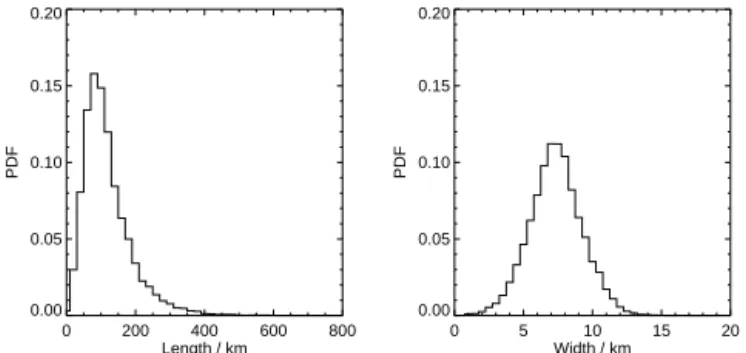
Figure 5.Probability density function of the effective length and
width of the contrails studied.
and night lead to stronger SW forcing through the RRUMS warm bright surface flux overestimation. Statistical analysis of the irradiance of the surrounding pixels such as taking the mean irradiance and the values within one standard deviation without any further assumption on the background behaviour also lead to errors. In this case, the contribution of contrail pixels not detected as such by ACTA biased the background forcing calculations. Different distances to the contrail pixels and/or pixel irradiance of previous images were also unsuc-cessfully considered.
When exclusively using satellite imagery for the assess-ment of the contrail RF, the impossibility of directly retriev-ing the background contribution arises. The high variability of scenes – inherent to the problem we are trying to solve – does not allow for a simple straightforward solution. We find that our one-pixel approach and background assumption with a daytime and nighttime discrimination proved to be the best choice.
Energy forcing, EF, measures the amount of energy intro-duced into the Earth–atmosphere system during the lifetime of the contrail that forms along the flight path (Schumann et al., 2011, 2012a). It is an assessment of the climate impact by each contrail-producing flight in terms of the amount of energy per flight distance. EF can be calculated from our data set through Eq. (2), where RF is the radiative forcing,W is the contrail width and the integral runs from the moment of contrail formation (in our case, time of first observation in the satellite image) until dissipation. The EF is computed in units of energy per unit length.
EF=
Z
lifetime
RF(t, s)·W (t, s)dt (2)
A typical value for a contrail whose lifetime is 10 000 s, has a 1 km width and produces a net RF of 10 W m−2 is
100 GJ km−1 (Schumann et al., 2012a). However, the
vari-ability of the EF is very large; it can reach several thou-sand GJ km−1warming or cooling for single route segments
because of weather-dependent RF values and because of dif-ferent contrail lifetimes (Matthes et al., 2012).
0 5 10 15 20
Lifetime / h 1
10 100 1000
Nr. of contrails
Figure 6.Lifetimes of the contrails studied. Dashed line:e-folding
time 3 h. Dotted line:e-folding time 1 h.
3 Results
The data set consists of 25 179 contrail events issued from the 2375 contrails detected by the CDA on Terra/MODIS and tracked by ACTA on MSG/SEVIRI (Rapid Scan Ser-vice). The following information has been retrieved for each contrail and contrail event: location, length, width, radiative forcing (RF), energy forcing (EF), optical thickness (τ) and contrail top altitude.
3.1 Location
Figure 7.Probability density function of the optical thickness of the tracked contrails. The dashed line represents the probability density function of the gamma distribution (see text).
3.2 Length and width
The characteristic length and width of each contrail event is shown in Fig. 5. Contrail length is computed as the dis-tance between the two most distant pixels of the scene. The average length, 130 km (standard deviation, 72 km), is con-sistent with the mean path length of ice supersaturated re-gions in the upper troposphere/lower stratosphere (UTLS) region of 150 km (Gierens and Spichtinger, 2000). Iwabuchi et al. (2012) retrieved a considerably longer average contrail length of 264 km (standard deviation 294) for contrails over the Northern Hemisphere using MODIS. However, the PDF of their contrails has a mode at 50–100 km, as do the contrails in our data set.
The contrail width is computed as the total contrail area covered by the contrail pixels divided by the length. Hence, in certain cases, this effective width may lead to a value narrower than the pixel width itself. The average width ob-tained here is 7.8 km (standard deviation, 2.0 km). It is possi-ble to compare our findings with the study by Duda et al. (2013) where three different masks were implemented to examine contrail coverage. The widths they derived ranged from 3.75 km (most restrictive mask, exclusively linear con-trails) to 5.23 km (some contrail cirrus included). Our result show larger widths not only because the pixel size is larger (SEVIRI vs. MODIS), but also because more contrail cir-rus clouds are considered. Assuming an initial width of 60 m and a spreading rate of 50 m min−1, our average width is
reached slightly after 2.5 h. The spreading rate observed by Duda et al. (2004) in the case study over the Great Lakes, 2.7 km h−1, applied to our case would mean that the 7.8 km
average width is reached after 2.8 h. Please note that the find-ings described in this paper apply to this subset of contrails.
3.3 Lifetime
The most important result that can be obtained with the help of ACTA is the contrail lifetime. Until now, it was possible to characterise linear contrails but little was known about their temporal evolution, with the exception of case studies such as the ones mentioned earlier. Figure 6 shows the distribu-tion of the contrail lifetimes, along with thee-folding times corresponding to 1 (dashed) and 3 h (dotted). The average lifetime of the complete data set is 54.6 min. This value in-cludes the large number of contrails that are not tracked past their initial stages due to the difficult scene characteristics.
Excluding the contrails that, due to scene (or ACTA) lim-itations, cannot be tracked in more than one scene, the aver-age lifetime is 70.5 min. Thee-folding times lines show that a typical value for the contrails that can be tracked lies in the 2 h range.
3.4 Optical thickness and cloud height
The combination of ACTA and COCS provides information on the optical thickness, τ, and the altitude of the tracked contrails. Figure 7 shows the PDF ofτ values of the tracked contrails. The meanτ in our data set is 0.34 with a median value of 0.24. Although the minimum reliableτ issued from COCS is 0.1, 17 % of all contrail pixels had a COCSτ below 0.1. Only 2 % of the pixels have aτ >1. The PDF behaviour is similar to the Iwabuchi et al. (2012) findings, whereτ was retrieved directly from CALIOP data even though they take into account only linear contrails. The average τ they re-trieved is 0.19. For the sake of comparison with future works, the probability density function of a fitted gamma distribu-tion defined as follows (Eq. 3) is also shown.
f (τ )=τ
γ−1e−τ/µ
µγŴ(γ ) (3)
Ŵis the gamma function, and the shape,γ, and scale,µ, pa-rameters in our case are 1.5 and 0.151, respectively. Bedka et al. (2013), using a modified CDA on Aqua/MODIS, re-trieved an averageτof linear contrails of 0.216. Minnis et al. (2013) closely analysed 11 contrail outbreaks using Terra and Aqua MODIS data and derived τ values of contrail cirrus ranging from 0.32 to 0.43 andτvalues of linear contrails be-tween 0.13 and 0.17. The in situ measurements ofτtaken by Voigt et al. (2011) are also consistent with our findings. Fur-ther methods of deriving optical thickness show smaller aver-age values: the model simulations by (Kaercher et al., 2010) yield mean values typically around 0.1 due to the amount of sub-visible contrails considered.
0.0 0.2 0.4 0.6 0.8 1.0 1.2 τ
0.0 0.1 0.2 0.3 0.4 0.5 0.6
0 2 4 6 8 10
τ x width / km 0.0
0.1 0.2 0.3 0.4
6 8 10 12 14 16 18 Height / km
0.00 0.05 0.10 0.15 0.20 0.25
Figure 8.Histograms of the optical depth,τ (left), the product ofτ and width (centre) and the height above sea level (right) for different
contrail ages. Solid line: younger than 30 min; dashed: 3 to 5 h; dotted: longer than 8 h.
Day, water
-20 0 20 40 60 80 100 RF LW / (W/m2) 0
200 400 600
Nr. of contrails
Day, land
-20 0 20 40 60 80 100 RF LW / (W/m2) 0
50 100 150 200 250
Nr. of contrails
Night, water
-20 0 20 40 60 80 100 RF LW / (W/m2) 0
50 100 150 200 250
Nr. of contrails
Night, land
-20 0 20 40 60 80 100 RF LW / (W/m2) 0
20 40 60 80 100
Nr. of contrails
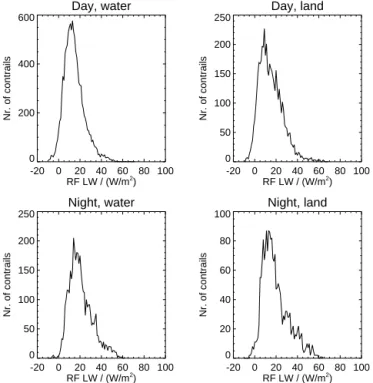
Figure 9.Frequency of occurrence of LW radiative forcing for the
tracked contrails.
young (linear) contrails shows the expected behaviour: linear contrails are mainly optically thin. With time (dashed line), contrails allowed to grow under favourable atmospheric con-ditions adopt a less steep distribution curve. Most of the old-est contrails under study (dotted line) have a very lowτ. A secondary maximum in the distribution is caused by contrails within clusters or growing into pre-existing cirrus clouds. In those cases,τ is strongly influenced by the surroundings and no general conclusions can be drawn. The main observation, the optical thickness decrease with age, is expected and has been shown in numerical simulations such as Unterstrasser and K. Gierens (2010): the longer a contrail lives, the more it is likely to spread, and in the long term it will be optically thinner.
Day, water
-150 -100 -50 0 50 100 RF SW / (W/m2) 0
50 100 150 200 250 300
Nr. of contrails
Day, land
-150 -100 -50 0 50 100 RF SW / (W/m2) 0
50 100 150
Nr. of contrails
Figure 10. Frequency of occurrence of daytime SW RF for the
tracked contrails. Nighttime SW RF (not shown) is 0.
To stress this result we show the product of optical thick-ness and width in Fig. 8 (centre) for the same three cate-gories. It can be seen that, on average, the longer a contrail lives, this product becomes lower in spite of the increasing width.
The last graph on the right in Fig. 8 shows the relationship between altitude and contrail age. The altitude is consistent with expected values: mean value 11.7 km, with 0.9 km stan-dard deviation. Similar values are shown by Iwabuchi et al. (2012): 10.9 km with a standard deviation of 1 km. The tem-poral evolution of the altitude does not show any conclusive results on the fall rates. The vertical resolution provided by COCS is insufficient to resolve fall speeds. The top altitude retrieval of the COCS algorithm presents a standard devia-tion of 750 m whereas the observadevia-tions of contrail fall rates lie in the 0.045 m s−1range (Duda et al., 2004).
3.5 Radiative forcing and energy forcing
over--1.0 -0.5 0.0 0.5 1.0 cos(SZA)
0.000 0.005 0.010 0.015 0.020
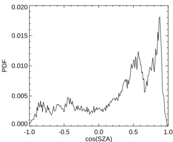
Figure 11.Probability density function of the cosine of solar zenith
angle corresponding to the contrails in the data set.
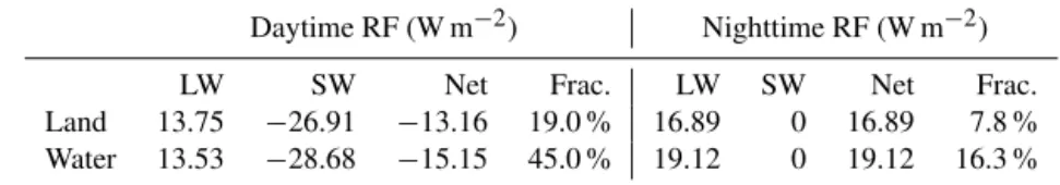
pass time and does not reproduce the actual traffic pattern. Moreover, the criterion for background assessment at day-time is different than the nightday-time criterion, so showing a mean value from the data set would be misleading. Instead, the analysis focuses on two different backgrounds (land/sea) under two different conditions (day/night). The median value is chosen instead of the mean in order to use a parameter that is more representative of the distribution and less sensitive to outliers. It can be seen that the net daytime forcing is the bal-ance between two large quantities of different signs where the SW contribution outweighs the LW leading to a net ra-diative cooling. At nighttime there is no reflected solar radi-ation, which causes contrails to have a net radiative warm-ing effect. Please note that followwarm-ing contrails have been ex-cluded from the results: those extending over both land and water backgrounds and those under extreme solar zenith an-gles (dusk/dawn).
The variability of the LW forcing is large, as seen on the frequency distribution plots in Fig. 9. The median value here derived for the LW RF ranges between 13 and 19 W m−2
de-pending on the time of the day and the background. Previ-ous works show similar forcings, such as in Palikonda et al. (2005) (12 to 27 W m−2, from MODIS/AVHRR data).
How-ever, direct comparison with previous works must be car-ried out carefully because RF varies greatly depending on the surroundings and on the time of the day. Model-based stud-ies on the LW such as Meerkoetter et al. (1999) and Stuber and Forster (2007) consider that the mean LW forcing easily reaches 40 or 50 W m−2over a cloud-free continental
mid-latitude summer atmosphere. More recent studies involving contrails detected by the MODIS instrument and modelled backgrounds range between 11 and 18 W m−2(Spangenberg
et al., 2013).
-1.0 -0.5 0.0 0.5 1.0
cos(SZA) -60
-40 -20 0 20 40 60
RF / W/m
2
Figure 12.Radiative forcing (blue: LW, red: SW) vs. cosine of the
solar zenith angle (SZA) corresponding to the contrails in the data set.
The distribution of the SW RF also presents large vari-ability (see Fig. 10). The median SW RF forcing be-tween−26 and−28 W m−2found here is slightly stronger
than expected. The reasons are twofold: overestimations by the RRUMS RSR algorithm over warm bright surfaces (Vázquez-Navarro et al., 2013) and the nature of our input data set. Shortwave RF depends on the solar zenith angle. Our contrails are found shortly before noon, which leads to higher SW RF values (see Figs. 11 and 12). The RF distribu-tion peaks around−20 W m−2and quickly decreases.
The low fraction of negative RF LW values (2.6 %) and positive RF SW values (2 %) present in the RF distribution plots evidences the difficulty of choosing the right back-ground pixels.
The behaviour of the RF with respect to the optical thick-ness is shown in Fig. 13 for both the LW (blue) and the SW (red) ranges. The darker colours indicate a higher number of occurrences. Despite the great variability of the data set, it can be clearly seen that for higherτ values both forcings increase. When τ approaches 0, the forcings tend to zero. This is also shown by the results of a parameterised analyti-cal model described in Schumann et al. (2012b).
The energy forcing is shown in Table 2. The large amount of energy inserted in (or removed from) the at-mosphere through the presence of a contrail until it dissi-pates can be observed. The observed energy forcing exceed-ing 500 GJ km−1 shows that a few big contrails contribute
Table 1.Radiative day- and nighttime forcing of the tracked contrails (median values). In percent, the fraction of contrails in each case.
Daytime RF (W m−2) Nighttime RF (W m−2)
LW SW Net Frac. LW SW Net Frac.
Land 13.75 −26.91 −13.16 19.0 % 16.89 0 16.89 7.8 %
Water 13.53 −28.68 −15.15 45.0 % 19.12 0 19.12 16.3 %
Table 2.Day- and nighttime energy forcing. In percent, the fraction of contrails in each case.
Daytime EF (GJ km−1) Nighttime EF (GJ km−1)
LW SW Net Frac. LW SW Net Frac.
Land 267.87 −610.02 −342.15 18.7 % 269.83 0 269.83 11.3 %
Water 290.30 −875.23 −584.93 48.6 % 403.04 0 403.04 21.3 %
0.0 0.2 0.4 0.6 0.8 1.0
τ
-60 -40 -20 0 20 40 60
LW RF / W/m
2
0.0 0.2 0.4 0.6 0.8 1.0
τ
-60 -40 -20 0 20 40 60
SW RF / W/m
2
Figure 13.Radiative Forcing vs.τ. Red: SW; blue: LW
4 Summary and Conclusions
We have been able to track in time successfully and for the first time over 2300 contrails corresponding to over 25 000 events. This has been done combining the CDA detection (Mannstein et al., 1999) and the ACTA tracking (Vázquez-Navarro et al., 2010) algorithms. The obtained data set com-prises short- and long-lived contrails in linear and non-linear stages, resembling nature. The lack of similarity with the air traffic pattern is mainly due to two reasons: the fact that the tracked contrails only issue from Terra/MODIS overpasses and the known limitations in the detection efficiency of CDA. There is known bias towards wider and thicker contrails. Contrail clusters are present in the data set, but may be un-derrepresented.
Nevertheless, the data set constitutes a representative se-lection of contrails under different formation conditions and with different properties from satellite images and – thanks to the automatic tracking – the selection includes for the first time clouds that would otherwise be considered natural. Some of the tracked contrails have properties differing from those reported for linear contrails in the past, in particular we found many optically thick and geometrically wide contrails. This stresses the importance of considering both linear
con-trails and contrail cirrus together when studying the radiative impact of air-traffic-induced cloudiness.
Several contrail properties have been derived, either di-rectly by using ACTA (width, length, lifetime) or by combin-ing it with other algorithms such as COCS (optical thickness and contrail top altitude) or RRUMS (radiative forcing and energy forcing). The combination with further algorithms to retrieve ice water content or particle size could provide valu-able information on the contrail aging process. Information on the contrail temperature is also necessary for further stud-ies.
The findings constitute a valuable data set in which several physical properties of (satellite observed) contrails during their lifetime are analysed. An average contrail/contrail cir-rus in the data set has an effective width of 8 km and a length of 130 km. This length is compatible with the extension of the ice supersaturated layers (Gierens and Spichtinger, 2000). The top altitude lies in the expected range: 11.7 km. The meanτ is 0.34.
Comparing with the recent study from Iwabuchi et al. (2012), it can be seen that our data set is formed by shorter contrails (130 km vs. 260 km) that are optically thicker (0.34 vs. 0.19). The main difference between both data sets is the type of contrail under study and the areas under considera-tion. Our optical thickness retrieval has a lower boundary of 0.1, and in their data set 34 % of contrails haveτ below 0.1. The recent analysis of Bedka et al. (2013) gave aτ value of 0.2, with 21 % below 0.1. The study of contrail outbreaks by Minnis et al. (2013) show optical thicknesses for contrail cir-rus ranging from 0.32 to 0.43, consistent with our findings.
con-trast with the background) and to a sub-pixel width. Several case studies for instruments with a spatial resolution simi-lar to SEVIRI (for example Duda et al., 2004, using GOES imagery) have pointed out that this missing time is close to 1 h. This extra hour is consistent with the fact that the aver-age lifetime of the tracked contrails is around 1 h (plus the additional initial period not visible from the satellite plat-form) and the average width is reached after around 2.5 h. Our findings are also in agreement with Graf et al. (2012), who observed maximum cirrus contrail cover over the North Atlantic between 2.1 and 4.1 h after passage of air traffic.
The radiative forcing derived is in agreement with previ-ous works. In order to compute the contrail radiative forcing, different assumptions on the shortwave and long-wave out-going flux density have been tested and discussed. As a con-sequence, no net value is shown but contrails have been clas-sified in four categories combining day/night conditions and land/ocean backgrounds. A similar classification of the op-tical thickness and height presents similar values in all four categories and is therefore not shown. RF LW median val-ues for the different situations range from 13 to 19 W m−2
and RF SW is around−27 W m−2. There are differences
be-tween day- and nighttime and also bebe-tween land and water backgrounds. All RF distributions show a main peak and a long tail. This stresses their large variability of nature and the need to carefully consider the correct contrail-free state of the atmosphere. An additional analysis of the relationship between the forcing and τ shows, as expected, that the RF is low when the optical thickness approaches 0 but gains im-portance with increasing τ. A better characterisation of the distribution of the RF values is crucial to model approaches. Due to the nature of the analysis carried out, it is not possible to derive a representative estimate for the net RF value. The different criteria for day- and nighttime background pixel se-lection prevent from a direct RF SW + RF LW comparison.
Unlike the energy forcing that directly gives informa-tion about the average effect of contrails in the atmosphere throughout their lifetime, the radiative forcing is not related to the lifetime of contrails. However, estimates of the global contrail radiative forcing are linked to the contrail cover-age, which is inherently related to contrail lifetime. Tracking methods such as ACTA, be they on their own or in combi-nation with other algorithms, provide very valuable informa-tion about not only contrail physical properties but also their evolution. The results can help reduce the large uncertainties still existing on the effect of aviation-induced cloudiness in climate.
Acknowledgements. This work contributes to the DLR project
WeCARE. The authors would like to thank Ulrich Schumann, Kaspar Graf and Luca Bugliaro for their comments and remarks. We thank Bernhard Mayer for his assistance with libRadtran for RRUMS. This paper is dedicated to the memory of our colleague and mentor Hermann Mannstein.
The article processing charges for this open-access publication were covered by a Research
Centre of the Helmholtz Association.
Edited by: S. Buehler
References
Atlas, D., Wang, Z., and Duda, D. P.: Contrails to cirrus: morphol-ogy, microphysics, and radiative properties, J. Appl. Meteorol., 45, 5–19, 2006.
Bakan, S., Betancor, M., Gayler, V., and Grassl, H.: Contrail fre-quency over Europe from NOAA-satellite images, Ann. Geo-phys., 12, 962–968, 1994,
http://www.ann-geophys.net/12/962/1994/.
Bedka, S. T., Minnis, P., Duda, D. P., Chee, T. L., and Palikonda, R.: Properties of linear contrails in the Northern Hemisphere derived from 2006 Aqua MODIS observations, Geophys. Res. Lett., 40, 772–777, doi:10.1029/2012GL054363, 2013.
Burkhardt, U. and Kaercher, B.: Global radiative forcing from contrail cirrus, Nature Climate Change, 1, 54–58, doi:10.1038/nclimate1068, 2011.
Duda, D. P., Minnis, P., Nguyen, L., and Palikonda, R.: A case study of the development of contrail clusters over the Great Lakes, J. Atmos. Sci., 61, 1132–1146, 2004.
Duda, D. P., Minnis, P., Khlopenkov, K., Chee, T. L., and Boeke, R.: Estimation of 2006 Northern Hemisphere contrail cover-age using MODIS data, Geophys. Res. Lett., 40, 612–617, doi:10.1002/grl.50097, 2013.
Gierens, K. and Spichtinger, P.: On the size distribution of ice-supersaturated regions in the upper troposphere and lowermost stratosphere, in: Ann. Geophys., 18, 499–504, Springer, 2000. Graf, K., Schumann, U., Mannstein, H., and Mayer, B.: Aviation
induced diurnal North Atlantic cirrus cover cycle, Geophys. Res. Lett., 39, L16804, doi:10.1029/2012GL052590, 2012.
Harries, J. E., Russell, J. E., Hanafin, J. A., Brindley, H., Futyan, J., Rufus, J., Kellock, S., Matthews, G., Wrigley, R., Last, A., Mueller, J., Mossavati, R., Ashmall, J., Sawyer, E., Parker, D., Caldwell, M., Allan, P. M., Smith, A., Bates, M. J., Coan, B., Stewart, B. C., Lepine, D. R., Cornwall, L. A., Corney, D. R., Ricketts, M. J., Drummond, D., Smart, D., Cutler, R., Dewitte, S., Clerbaux, N., Gonzalez, L., Ipe, A., Bertrand, C., Joukoff, A., Crommelynck, D., Nelms, N., Llewellyn-Johnes, D. T., Butcher, G., Smith, G. L., Szewczyk, Z. P., Mlynczak, P. E., Slingo, A., Allan, R. P., and Ringer., M. A.: The Geostationary Earth Radia-tion Budget Project, B. Am. Meteorol. Soc., 86, 945–960, 2005. Iwabuchi, H., Yang, P., Liou, K. N., and Minnis, P.: Phys-ical and optPhys-ical properties of persistent contrails: Clima-tology and interpretation, J. Geophys. Res., 117, D06215, doi:10.1029/2011JD017020, 2012.
Kaercher, B., Burkhardt, U., Ponater, M., and Fromming, C.: Im-portance of representing optical depth variability for estimates of global line-shaped contrail radiative forcing, P. Natl. Acad. Sci. USA, 107, 19181–19184, 2010.
Kox, S., Bugliaro, L., and Ostler, A.: Retrieval of cirrus cloud opti-cal thickness and top altitude from geostationary remote sensing, Atmos. Meas. Tech., 7, 3233–3246, doi:10.5194/amt-7-3233-2014, 2014.
Lee, D. S., Fahey, D. W., Forster, P. M., Newton, P. J., Wit, R. C. N., Lim, L. L., Owen, B., and Sausen, R.: Aviation and global climate change in the 21st century, Atmos. Environ., 43, 3520– 3537, doi:10.1016/j.atmosenv.2009.04.024, 2009.
Lee, T. F.: Jet contrail identification using the AVHRR infrared split window, J. Appl. Meteorol., 28, 993–995, 1989.
Loeb, N. G., Kato, S., Loukachine, K., and Manalo-Smith, N.: An-gular Distribution Models for Top-Of-Atmosphere radiative flux estimation from the Clouds and the Earth’s Radiant Energy Sys-tem Instrument on the Terra satellite. Part I: Methodology, J. At-mos. Ocean. Tech., 22, 338–351, 2005.
Mannstein, H. and Schumann, U.: Aircraft induced contrail cir-rus over Europe, Meteorol. Z., 14, 549–554, doi:10.1127/0941-2948/2005/0058, 2005.
Mannstein, H., Meyer, R., and Wendling, P.: Operational Detection of Contrails from NOAA-AVHRR-Data, Int. J. Remote Sens., 20, 1641–1660, 1999.
Matthes, S., Schumann, U., Grewe, V., Frömming, C., Dahlmann, K., Koch, A., and Mannstein, H.: Climate optimized air transport, in: Atmospheric Physics, 727–746, Springer, 2012.
Meerkoetter, R., Schumann, U., Doelling, D. R., Minnis, P., Na-jakima, T., and Tsushima, Y.: Radiative forcing by contrails, Ann. Geophys., 17, 1080–1094, 1999,
http://www.ann-geophys.net/17/1080/1999/.
Meyer, R., Mannstein, H., Meerkoetter, R., Schumann, U., and Wendling, P.: Regional radiative forcing by line-shaped con-trails derived from satellite data, J. Geophys. Res., 107, D10, doi:10.1029/2001JD00426, 2002.
Meyer, R., Buell, R., Leiter, C., Mannstein, H., Marquart, S., Oki, T., and Wendling, P.: Contrail observations over Southern and Eastern Asia in NOAA/AVHRR data and comparisons to con-trail simulations in a GCM, Int. J. Remote Sens., 28, 2049–2069, 2007.
Minnis, P., Ayers, J. K., Palikonda, R., and Phan, D.: Contrails, Cir-rus Trends, and Climate, J. Climate, 17, 1671–1685, 2004. Minnis, P., Palikonda, R., Walter, B. J., Ayers, J. K., and Mannstein,
H.: Contrail properties over the eastern North Pacific from AVHRR data, Meteor. Z., 14, 515–523, 2005.
Minnis, P., Bedka, S. T., Duda, D. P., Bedka, K. M., Chee, T., Ayers, J. K., Palikonda, R., Spangenberg, D. A., Khlopenkov, K. V., and Boeke, R.: Linear contrail and contrail cirrus properties deter-mined from satellite data, Geophys. Res. Lett., 40, 3220–3226, 2013.
Palikonda, R., Minnis, P., Duda, D. P., and Mannstein, H.: Contrail coverage derived from 2001 AVHRR data over the continental United States of America and surrounding areas, Meteor. Z., 14, 515–523, 2005.
Schmetz, J., Pili, P., Tjemkes, S., Just, D., Kermann, J., Rota, S., and Ratierk, A.: An introduction to Meteosat Second Generation (MSG), B. Am. Meteorol. Soc., 83, 977–992, 2002.
Schumann, U. and Graf, K.: Aviation-induced cirrus and radiation changes at diurnal timescales, J. Geophys. Res., 118, 2404–2421, 2013.
Schumann, U., Graf, K., and Mannstein, H.: Potential to reduce the climate impact of aviation by flight level changes, in: 3rd AIAA Atmospheric and Space Environments Conference, AIAA paper 2011-3376, doi:10.2514/6.2011-3376, 2011.
Schumann, U., Graf, K., Mannstein, H., and Mayer, B.: Con-trails: Visible aviation induced climate impact, in: Atmospheric Physics, 239–257, Springer, 2012a.
Schumann, U., Mayer, B., Graf, K., and Mannstein, H.: A paramet-ric radiative forcing model for contrail cirrus, J. Appl. Meteor., 51, 1391–1406, 2012b.
Spangenberg, D. A., Minnis, P., Bedka, S. T., Palikonda, R., Duda, D. P., and Rose, F. G.: Contrail radiative forcing over the North-ern Hemisphere from 2006 Aqua MODIS data, J. Geophys. Res., 40, 595–600, doi:10.1002/grl.50168, 2013.
Spichtinger, P., Gierens, K., and Read, W.: The global distribution of ice-supersaturated regions as seen by the Microwave Limb Sounder, Q. J. R. Meteoroloc. Soc., 129, 3391–3410, 2003. Stocker, T. F., Qin, D., Plattner, G.-K., Tignor, M., Allen, S. K.,
Boschung, J., Nauels, A., Xia, Y., Bex, V., and Midgley, P. M.: Climate change 2013: The physical science basis, Intergovern-mental Panel on Climate Change, Working Group I Contribution to the IPCC Fifth Assessment Report (AR5)(Cambridge Univ Press, New York), 2013.
Stuber, N. and Forster, P.: The impact of diurnal variations of air traffic on contrail radiative forcing, Atmos. Chem. Phys., 7, 3153–3162, doi:10.5194/acp-7-3153-2007, 2007.
Unterstrasser, S. and Gierens, K.: Numerical simulations of contrail-to-cirrus transition – Part 1: An extensive parametric study, Atmos. Chem. Phys., 10, 2017–2036, doi:10.5194/acp-10-2017-2010, 2010.
Vázquez-Navarro, M., Mannstein, H., and Mayer, B.: An automatic contrail tracking algorithm, Atmos. Meas. Tech., 3, 1089–1101, doi:10.5194/amt-3-1089-2010, 2010.
Vázquez-Navarro, M., Mayer, B., and Mannstein, H.: A fast method for the retrieval of integrated longwave and shortwave top-of-atmosphere upwelling irradiances from MSG/SEVIRI (RRUMS), Atmos. Meas. Tech., 6, 2627–2640, doi:10.5194/amt-6-2627-2013, 2013.