Consumption-based macroeconomic models of asset pricing theory

UDC: 3.33 ISSN: 0013-3264

* U n i v e r s i t y o f B e l g r a d e , R e p u b l i c o f S e r b i a , E - m a i l : m a r i j a _ d j o r d j e v i c @ e k o f . b g . a c . r s

JEL CLASSIFICATION:

E 2 1 , G 1 2

ABSTRACT:

_{he family of}

consumption-based asset pricing models yields a

stochas-tic discount factor proportional to the

mar-ginal rate of intertemporal substitution of

consumption. In examining the empirical

performance of this class of models, several

puzzles are discovered. In this literature

review we present the canonical model, the

corresponding empirical tests, and

difer-ent extensions to this model that propose a

resolution of these puzzles.

KEY WORDS:

_{equity premium puzzle,}

stochastic discount factor, marginal rate of

intertemporal substitution, risk-free rate

puzzle, risk premium, volatility

DOI:10.2298/EKA1611007D

Marija Đorđević*

1. INTRODUCTION

Asset pricing theory follows two main streams. On the one hand there is the

Equilibrium Pricing approach in which agents maximize their objective

functions given their budget constraints, and after markets are cleared the

equilibrium prices emerge. The primitives of this type of models are the joint

distribution of the assets’ payoffs and the agents’ preferences. Since both of these

are not easily visible in financial markets, the advantage of the second approach,

the Arbitrage Pricing Theory, is that it does not require any knowledge of the

preferences of the agents. This approach is based on the possibility of replicating

the payoff of one asset by creating a portfolio of other assets that have already

been priced. It follows that the price of such an asset should be equal to the price

of the replicating portfolio.

Equilibrium pricing comprises many different models that postulate different

preferences of agents. For example, the Capital Asset Pricing Model assumes

that agents have preferences defined over risk and return so that the agents are

the mean-variance optimizers. In this paper we are going to focus on the family

of models in which agents have preferences over consumption and/or their

wealth. Robert Lucas introduced a particular theoretical framework with a

one-good, pure exchange economy with continuum of consumers that are identical

in terms of their preferences and endowments (Lucas 1978), but the model can

be extended to the economy that satisfies conditions which allow the existence

of a representative agent. The agents decide how much to consume and how

much to save, so that the pricing formula comes out as a result of their

optimization. In this type of models, consumption is the key endogenous

variable in the economy and the calibration requires looking at the

macroeconomic variables.

evolution of asset pricing literature inside this particular theoretical framework,

and describe the puzzles that emerge from it.

The rest of the paper is organized as follows. The next section studies the

baseline Lucas (1978) model of joint consumption and investment choice in a

pure exchange economy and examines the equilibrium pricing equations.

Section 3 presents the applications of the model, defines the most important

asset pricing puzzles that arise from the consumption asset-pricing framework,

and briefly describes the theoretical directions towards solving the puzzles.

Section 4 concludes.

2. THE MODEL

The economy is populated by a continuum of homogeneous agents, but we can

as well relax this assumption by allowing the agent heterogeneity under the

conditions specified in Rubinstein (1974), which make aggregation into a

representative agent possible. We consider a pure exchange economy, with one

homogeneous good that serves as a numeraire.

Let

(Ω,

࣠

,P) denote the probability space. There are n productive units that

produce the good, such that at time t the productive unit i produces output yi,t.

Output vector at time t is given by yt = (y1,t,...,yn,t). The state variable yt is adapted

to the filtration {Ft} t=0,1,..,∞. Production is exogenous and stochastic and it is

assumed that the output vector process is a Markov chain with a time-invariant

transition-conditional probability distribution function G

ǣԹ

ൈ Թ

՜ Թ

:

(1)

Assuming that

ݕ

has a stationary distribution, the unconditional distribution is

given by:

߮ሺݕԢሻ ൌ ׬ ܩሺݕ

_{ǡ ݕሻ݀߮ሺݕሻ}

_{. (2)}

what share of ownership of each productive unit to acquire. Buying a share of

the productive unit today entitles the agent to the same share of the output of

that productive unit in the next time period. Output is perishable, which means

that it cannot be stored for consumption in later periods, which puts a boundary

on the current consumption:

. (3)

The representative agent’s preferences are described by the utility function

����

� �

, which is bounded, continuous, at least twice differentiable,

increasing, and strictly concave with U (0) = 0. He wishes to maximize the

expected value of his utility function:

(4)

By specifying the utility function in this way, we impose the time-separability of

the consumer’s preferences. The time preference is manifested only through the

impatience factor β, and the utility derived from the consumption at period

t

does not depend on the consumption from any time period other than

t

_{. Also,}

with preferences defined as above, we do not have the dependence of utility of

consumption on the particular state of the nature realization. This is the

property of the state-independence of utility function.

Let

be the vector of the agent’s beginning-of-period share

holdings at time t. If

�

is the prevailing price of one share of productive unit at

time

t

_{, his budget constraint becomes:}

�

����

���

�� � �

���

����

���

.

(5)

2.2. Equilibrium

Before we give a formal definition of the equilibrium in this economy, we

explain how the rational expectation equilibrium is established. One of the

elements of equilibrium characterization is the equilibrium price, which is

stochastic, given that it is a function of the state variable

�

. The quantity

���

�

stands for the price of the production unit

i

_{when the economy is in the state}

�

_.

By knowing the conditional probabilities of the economy changing from one

state to another, we can fully specify the dynamic stochastic behaviour of the

equilibrium price.

At time

t

, the agent has two choice variables,

�

and

�

. In making decisions

he is taking into account how prices change over time as a function of the state

of the economy. Equilibrium decision rules are

�

� � ����

� �

� �

�

and

����

� � �����

� ��

� ��

�

. These decision rules define how much the agent optimally

consumes (invests in productive unit shares) at period

t,

_{given the state of the}

economy, the size of the ownership of production units at the beginning of the

period, and the prevailing price. Given these decision rules, the market clearing

conditions yield the equilibrium price function. In the Rational Expectation

Equilibrium framework, the resulting price coincides with the price that the

consumer conjectured when he was solving his optimization problem.

The formal definition of the equilibrium is based on the dynamic programming

principle, where the representative agent’s objective function is restated in a

recursive form by writing the Bellman equation.

Definition.

_{(Lucas 1978). An equilibrium is a continuous function}

���� ∶

���

_{� ��}

_{and a continuous bounded function}

_{���� ������}

_{� ��}

_{� �}

_such

that:

(6)

such that

for

, where

� �

is a vector with all the elements exceeding one and for

each

�

,

is attained by

� � ∑

�

and

, where stands for the

vector of ones.

The first part of the statement refers to the representative agent’s optimal wealth

allocation given the price behaviour. There is also a condition which does not

allow negative consumption and the one which keeps the share positions finite

given that the price may take a zero value. The last part refers to the market

clearing conditions.

The non-negativity constraint on consumption can be omitted by assuming that

Inada conditions hold. Apart from the concavity and monotonicity properties of

the utility function that are already assumed, Inada conditions require that:





.

Let us consider first the maximization part of the problem. Let

�

stand for the

agent’s wealth at time

t,

_{which comes from the market value of the share}

ownership at time

t

and the dividend

�

that is claimed by the agent. It is given

by:

�

� ��

� �

��

�� � �

(7)

The time-separability of preferences allows the dynamic programming

approach and using the Bellman equation method. Since the state variable

�

summarizes the investor’s information set

�

,

we can use the notation

� ��

��

�

for the value function instead of

� ��

��

�

.

(8)

such that

Differentiating the Lagrangian function yields the first order conditions:

�� ���

�

������

���

� �

� �

(9)

��

��

� �

� �

� �

� ���

� � �

We write only the price as an explicit function of the state, even though the

consumption

c

, the share positions

z

and the shadow prices

λ

are also

functions of the state, because the investor makes his optimal decisions

contingent on the state of the economy. Since

W

=

z

·

(

p

(

y

) +

y

), the

partial derivative of the wealth in the next period with respect to the share

position the investor buys today is equal to:

�����

�����

� ���

� � �

(10)

Notice that in order to make

W

an explicit argument of the value function

J,

we substitute

c

=

W

− z

· p

(y

) from the constraint into the utility function

part of the objective

J

. From there it follows that

���

�

������

���

and it

also holds for the partials from the next period. Since value function

J

represents the total discounted utility, given that the investor made the

optimal consumption and investment decisions, this condition requires that

the marginal total utility of current wealth equals the marginal current

utility of consumption. The marginal utility of one unit of consumption

good spent today must be the same as the marginal value of one unit of

consumption good saved and spent some time in the future. The investor

has to be indifferent between purchasing the tree and selling the tree and

using the proceedings for the current consumption.

(11)

Mathematically, it is an Euler equation. The economic interpretation of this

equation is that the market price of an asset today is equal to the expected

value of the asset’s payoff tomorrow, adjusted by the ratio of marginal

utilities of consumption tomorrow and today. When marginal utility of

consumption tomorrow is low, it means that the consumption is high and

that the state’s payoff will be assigned lower weight in the pricing equation.

It is the opposite for the states with low consumption, where marginal utility

of the additional dividend is more valuable.

The increase in expected output increases the attractiveness of holding the

share of the asset, which pushes the price of the asset up. However, higher

expected output immediately means higher expected consumption, because

the consumption good is not storable and the agent consumes the entire

output in each state. If the expected consumption is high the marginal utility

is low, which has a negative effect on the asset price. What the resulting

effect of these two is depends on the particular shape of the utility function.

In this model the consumption good cannot be stored, so the equilibrium

price of the asset is adjusted to the point at which the investor consumes the

entire dividend in each period, which implies that we can substitute

ܿ

for

ݕ

as the argument of the marginal utility function in the equation (11).

The alternative way of expressing the Euler equation is to introduce pricing

kernel or stochastic discount factor that measures the willingness of the

investor to shift consumption between two dates and is equal to:

It is defined as a product of the marginal rate of intertemporal substitution

and the subjective discount factor. Substituting it into the pricing equation

(11) and expressing it in terms of the expected value

_yields:

���

� � ���

��

� �� ⋅ ����

� � �

���

� ��

(13)

The economic interpretation of this equation is that the price of the asset is

the expected value of the discounted value of future payoffs, with the

distinction that the payoffs are transformed into ‘utils’ by using the

stochastic discount factor.

The utility function is strictly increasing and the subjective discount factor is

strictly positive, which ensures that the stochastic discount factor is strictly

positive in each state of the world. This is an important property of the

stochastic discount factor, because it prevents the presence of arbitrage

opportunities in the economy. No arbitrage condition is stronger than the

requirement that the Law of One Price (LOOP) holds. We do not need the

stochastic discount factor to be positive in order for the financial markets to

obey LOOP, but only to have a linear pricing mechanism, which is the

condition equivalent to the mere existence of the stochastic discount factor.

For detailed proof of equivalence between LOOP and the linear pricing

mechanism on the one hand and the no arbitrage condition and strictly

positive stochastic discount factor on the other, see Cochrane (2005) or

Duffie (2001).

We can also express the pricing formula in terms of returns on assets. If we define

the gross return on holding the risky asset between periods

��

and

� � �

as:

�

�

(14)

then the pricing formula is given by:

� � �

��

��

� �� ⋅ �

�

(15)

1 _{In the rest of the text, the expected value conditional on the information from the state}

Now we turn to the Consumption Capital Asset Pricing Model derivation. We

are going to relax the assumption of the non-existence of the consumption good

storage technology. With this assumption, the optimal investor’s behaviour is to

consume the entire output. In that way the marginal rate of substitution and the

stochastic discount factor are both determined by the exogenous fluctuations in

the aggregate output. With the possibility of saving the output for future

periods, the investor’s consumption does not coincide with the aggregate output

in each state over the entire investment horizon. Consumption

�

is replaced in

equation (12) and the stochastic discount factor’s distribution is derived from

the distribution of the investor’s consumption.

First, we analyse the implications for the riskless asset, the one which has certain

constant payoff in every state of the world. That means that

�

is a constant

and can be taken out of the expectation operator in equation (15). That gives us

the expression for the riskless return in this economy:

�

�

���������������

(16)

The riskless gross return is just the reciprocal of the expected value of the

stochastic discount factor.

We now go back to the risky asset by using the Euler equation expressed in

terms of the gross returns as in the equation (15), and use the product rule to

obtain:

Ε

��

� � �

� �

������

� ���

��

� �

�

(17)

valuable to the investor. An asset that covaries positively with consumption is

poorly appreciated compared to the one that covaries negatively. This model

already provides the intuition that what matters is not the ‘individual’ but the

‘common’ risk in pricing the assets.

2.3. Asset Prices Without Bubbles

In order to prevent the possibility of creating a pricing bubble, the investor’s

maximization problem must satisfy the following transversality condition:

(18)

In order to see why this condition is important, we perform recursions on the

asset pricing equation (13), relying on the law of iterated expectations, which

yields:

(19)

If the transversality condition (18) holds, we have that the price of the asset is

equal to the expected value of the discounted dividend stream, but with the time

varying and stochastic discount factors.

(20)

assumption about the investor’s risk preferences, such as risk neutrality, the

Euler equation can collapse to the equilibrium price of the risky asset being

equal to the expected discounted value of the asset’s dividend stream with

constant discount factor. The risk-neutral investor is endowed with a linear

utility function, which implies that the marginal utility is constant and the

marginal rate of substitution is equal to one. The covariance term in (17) is

equal to zero and the implied pricing formula is:

(21)

In the next section we introduce more realistic assumptions regarding the

investor’s preferences and discuss the implications of the CCAPM application.

3. APPLICATION OF THE LUCAS MODEL

In this section we present Mehra and Prescott’s work on testing the Lucas model

using U.S. data on aggregate consumption, stock market returns, and returns on

government bonds. They show that this class of models cannot generate an

average annual equity premium of more than 6% without assuming an

unrealistically high value of the risk-aversion parameter. Prior to their work,

Hansen and Singleton (1982, 1983) used both the Generalized Method of

Moments with instrumental variables and the Maximum Likelihood Estimation

method on a canonical form of consumption-based model. They tested the

model on a time series of US monthly data on consumption growth and asset

returns, to find that the consumption-based pricing model is rejected. We

choose to present the Mehra and Prescott approach in greater detail, as they

introduce additional structure into the Lucas model and, in so doing, produce a

very simple test of the model’s empirical performance.

Beside the equity premium puzzle, we also present the risk-free rate puzzle

identified within this framework, and another test of the model validity which

requires much less of the model structure.

3.1. Equity Premium Puzzle

one productive unit. They make a slight variation in the model by changing

several assumptions. First, they observe that the U.S. per capita consumption

level exhibited a large increase over the period 1889-1978 that does not allow

assuming stationarity of the consumption process, as Lucas did. Instead of

assuming that the total output, with productivity exogenously given, follows the

Markov process, they assume that the growth rate of the aggregate output is a

Markov process. Second, they discretize the setup in terms of states. In each

period of time there is a finite number of states, described by a grid of values

that the dividend growth rate can take. In addition, they put structure on the

investor’s preferences by assuming the power utility function. For the sake of

consistency, we do not follow the paper closely and preserve the assumption of a

continuous-state economy. The results remain the same.

The economy is described as a pure exchange one, with one consumption good

produced by only one productive unit, i.e., there is only one Lucas tree in the

economy. Only one share of equity of the productive unit is traded, which

implies that the return on that asset is, at the same time, the return on the

market. Uncertainty in the economy is described by the probability space

��� �� ��

. The output produced by the productive unit

�

, which represents the

dividend received from the ownership over the productive unit, is exogenous

and stochastic with the growth rate being conditionally normally distributed

with mean µ

and variance σ

given the information available up to time t. We

define the growth rate as:

��� �

� ��

(22)

The investor has the power utility function:

(23)

them into the Euler equation for asset returns produces the following pricing

equation:

(24)

First we derive the implications for the risk-free rate between periods

t

_and

t+1

_.

Since

ܴ

is not random but a constant, it follows that the gross risk-free

return is equal to:

(25)

Since the representative investor consumes the entire output, the consumption

growth is conditionally normally distributed identically as the output growth,

and it follows that:

(26)

Let

ݎ

be the net risk-free return equal to

݈ܴ݊

. By taking the natural

logarithm of the inverse of the expression above we obtain:

(27)

Let us look at the comparative statics of expression (27):

•

The higher the impatience factor

ߠ

the higher the risk-free rate, because the

investor prefers to consume early; which is manifested in him reducing his

savings, thus having the risk-free rate increasing in the equilibrium.

•

When the consumer has a concave utility function, he wants to smooth his

consumption growth rate

the more he borrows today against future

consumption, and the equilibrium risk-free rate goes up.

•

High consumption growth volatility

�

makes the future consumption

more uncertain, which leads to the investor saving more, for precautionary

motives. As a consequence, in the equilibrium the risk-free return drops.

•

The risk aversion parameter γ magnifies the effect of change in the expected

growth rate of consumption and the consumption growth volatility. The

more risk-averse the investor, the more he tends to smooth the

consumption over time, but whether he borrows or saves more today

depends on the particular values of parameters

and

�

.

Now, let us turn to the risky asset with the gross return being a random variable

�

. It is assumed that

�

� � ���

is normally distributed, conditional on

the information from time

t

_{, with the mean}

�

���

��

_{and the variance}

���

����

�

. We start with the Euler equation by expressing the consumption

growth and the return

�

in exponential terms:

(28)

Calculating the expectation, taking the natural logarithm of both sides and

combining it with the expression for the risk-free rate yields:

(29)

In order to simplify the expression above we use the following two

approximations:

Ε

��

� � �

�

�����������

� � � Ε

��

� �

�

���

��

�

(30)

and

�

� � � �

(31)

(32)

In terms of the Sharpe ratio (equity premium per unit of risk), the pricing

formula becomes:

(33)

If we look at the equations (32) and (33), we see that the price of the risk is

governed by:

•

The risk aversion parameter γ, so that the higher the willingness of the

investor to smooth the consumption the higher the risk premium required.

•

The higher the correlation between the risky asset payoff and the

consumption growth the higher the discount at which the risky asset is

traded. If the economy is in a bad state, meaning that consumption growth

is small, the asset which pays off a lot in such a state is expensive compared

to the one that pays off a lot in a good state and the equity premium is small.

•

The higher the consumption volatility

�

�����

�

, the higher the price of

the risk, since holding the risky asset makes the consumption even more

unbalanced.

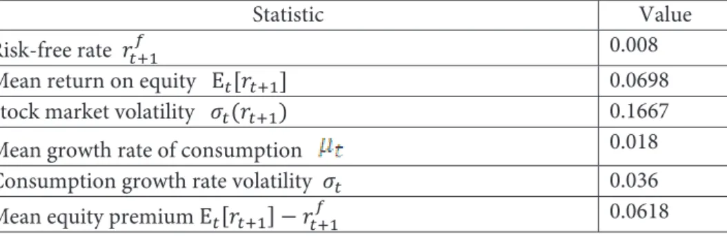
Table 1.

_{Mehra and Prescott (1985) U.S. Economy Sample Statistics (1889–1978)}

Statistic Value

Risk-free rate

�

0.008

Mean return on equity

���

0.0698

Stock market volatility

�

��

�

0.1667

Mean growth rate of consumption

0.018

Consumption growth rate volatility

�

0.036

Mean equity premium

Ε

��

0.0618

and Prescott (1985). Plugging these values into the expression for the equity

premium (32) and assuming that the correlation coefficient between

consumption growth and market return is equal to one (which ceteris paribus

gives the maximum equity premium) yields:

(34)

We need an excessively large relative-risk-aversion coefficient γ of at least 10.3

in order to rationalize the equity premium of 6.18 as evidenced on the stock

market. A number of studies reported in Mehra and Prescott (1985) found that

the risk aversion coefficient takes a value between one and two. The value that is

typically used in the literature is three. This discrepancy between the model

predictions and the stock market evidence is called the equity premium puzzle.

The equity premium puzzle is a puzzle of a quantitative nature. The models

described above are correct in predicting that the risky assets should on average

yield higher returns than bonds because of the higher risk attached. However,

they fail to predict the order of magnitude of the difference in returns,

compared to that which has been historically documented.

3.2. Risk-free Rate Puzzle

Philippe Weil (1989) invented the term ‘risk-free rate puzzle’ in an attempt to

resolve the equity premium puzzle by leaving the time-additive expected utility

framework and introducing the generalized non-expected utility specification,

which allows breaking the link between intertemporal elasticity of substitution

and risk aversion parameter, which are both functions of the curvature of the

utility function, and in the time-additive framework represent the inverse of

each other. Separating the risk aversion from the intertemporal substitution

explains the equity premium but risk-free rate puzzle emerges, because the

parameters that fit the equity premium yield the risk-free rate far higher than

the 0.8% observed in reality. In this paper we will expose the problem of the

risk-free rate puzzle in the framework of the Lucas model, i.e., we are going to

stay within the theoretical domain of the expected utility. If we plug the values

from Table 1 into the equilibrium expression for the risk-free rate as given in

equation (27), and if we take the parameter

ߜ

to be equal to 0.01005 so that the

The risk-aversion parameter that is used to rationalize the historical equity

premium is higher than 10. If we plug this value into the equation above we

obtain a risk-free rate equal to 12.52%, which is far above 0.8%, the risk-free rate

that characterized the US economy over the period 1889-1978.

3.3. Hansen-Jagannathan Bounds

In their completely non-parametric approach, which uses the minimum

structure possible, Hansen and Jagannathan (1991) find the admissible region

for the expected value and standard deviation of the stochastic discount factor.

In order to derive the lower bound of the volatility of the stochastic discount

factor, the only requirement is that the Law of One Price holds in financial

markets, which means that the stochastic discount factor exists as well as the

absence of arbitrage opportunities, which requires that the stochastic discount

factor is positive. For this purpose, we do not even need markets to be complete.

For the sake of simplicity, they focus on the unconditional version of the Euler

equation and use the risk-free return as a varying parameter, which is equal to

the inverse of the mean stochastic discount factor, in order to trace out the

lower bound of the volatility of SDF. Conditioning down pricing equations

creates a problem for empirical financial economists, since in reality it is

observed that the conditional moments of return and SDF distributions vary

over time because investors acquire new information. However, for the sake of

consistency we will present their result using the equations with conditional

moments.

Hansen and Jagannathan start from the general pricing equation (15), apply it to

the risk-free and the risky asset, and take the difference between the two to get:

Ε

��

��

� �

�� � �

(35)

By the product rule, the left hand side can be rewritten as

Ε

��

� ⋅

as a function of the correlation coefficient and after some simple algebraic

manipulation it follows that:

(36)

Since the absolute value of the correlation coefficient is bounded to be below or

equal to one, we get the lower bound for the volatility of the stochastic discount

factor:

�

�

�

�_����⋅�_����

(37)

This expression states that the lower bound for the stochastic discount factor

has to be at least equal to the Sharpe ratio of the stock market divided by the

gross risk-free rate. This bound serves as a test for any proposed asset pricing

model.

If we go back to the Mehra and Prescott’s stock market statistics in Table 1, we

can test the consumption-based asset pricing model derived under the

additional assumptions in Section 3. We get that:

�

�

1.06�8 � 1.008

_{0.1667 ⋅ 1.008 � 0.�677.}

Since the stochastic discount factor’s volatility in the consumption-based asset

pricing model is equal to the product of the volatility of the consumption

growth rate that is equal to 0.036 and the relative risk aversion coefficient

, it

requires the RRA coefficient to have a value of at least 10. As before, since this is

an unrealistically high coefficient value the consumption-based model did not

perform well.

3.4. Model Extensions

different specification of the utility function and introducing agent

heterogeneity into the model.

The models presented in this paper use the standard preference representation

characterized by time-separability, which implies that the coefficients of

elasticity of intertemporal substitution and the relative risk aversion are the

reciprocals of each other. Epstein and Zin (1989) introduced the class of

functions that describe the recursive preferences. The most important

characteristic is that the link between the two abovementioned coefficients is

broken and the risk-free rate puzzle can be mitigated, because one can achieve

higher expected market return by increasing the RRA coefficient, for the

purpose of solving the equity premium puzzle, without implying an

unrealistically high risk-free rate as a consequence.

An alternative class of models keeps the assumption of time-separability of

preferences, but assumes that the agent’s utility depends on a certain subsistence

level of consumption that serves as a benchmark. If the actual consumption level

drops below the subsistence level, it yields negative utility to the agent. This

stream of the literature was pioneered by Sundaresan (1989), Constantinides

(1990), and Abel (1990). The further advancement was made by Campbell and

Cochrane (1999). The basic idea is that the agents have formed a certain level of

habit which results in the effective risk aversion of a larger scale for the agent,

thus helping in the consumption-based model fitting the historical value of the

equity premium.

Models with heterogeneous agents (Mankiw 1986, Constantinides et al. 1996)

typically assume that the agents have individual income shocks that limit the

possibility of risk-sharing. With increasing cross-sectional volatility of

consumption in states where the asset returns are low, the assets’ risk premium

increases beyond the level yielded in the model with a representative agent.

Krueger and Lustig (2009) show that in an economy with a continuum of agents

the risk premium is not affected by the absence of an insurance market if the

aggregate shocks are distributed independently from the individual shocks, and

if the consumption growth is independently distributed over time.

component in return and consumption growth processes (Bansal et al. 2004), or

in the direction of studying the effect of different market frictions on the market

risk premium. For the latter, see He et al. (2005).

4. CONCLUSION

The consumption-based general equilibrium class of models provides a pricing

formula with very sharp intuition. The assets are priced in such a way that

buying an asset at a certain price incurs consequent marginal loss in utility from

current consumption equal to the discounted expected gain in utility of

consuming the asset’s payoff in the future. Even though this class of model is

correct in explaining the sign and the direction of the effects of one financial

variable on another, it fails in predicting the magnitude of the average return on

the stock market or the level and variation of interest rates. In terms of the

power of predicting the variables of interest, these models can be improved by

an alternative specification of agent’s preferences or by alternative assumptions

of different economic processes. The two most commonly used approaches are

to change the assumptions regarding the agent’s utility functions and to assume

the heterogeneity among agents.

REFERENCES

Abel, A. (1990). Asset Prices under Habit Formation and Catching Up with the Joneses. he

American Economic Review, Vol. 80, No. 2, pp. 38 – 42.

Bansal, R., Yaron A. (2004). Risks for the Long Run: A Potential Resolution of Asset Prizing

Puzzles. he Journal of Finance, Vol. 59, No. 4, pp. 1481–1509.

Breeden, D., T. (1979). An Intertemporal Asset Pricing Model with Stochastic Consumption and

Investment Opportunities. Journal of Financial Economics, Vol. 7, No. 3, pp. 265 – 296.

Campbell Y. J., Cochrane J. H. (1999). By Force of Habit: A Consumption-Based Explanation of

Aggregate Stock Market Behavior. he Journal of Political Economy, Vol. 107, No. 2, pp. 205 – 251.

Cochrane, J. H. (2005). Asset Pricing. Revised ed., Princeton University Press, New Jersey.

Constantinides, G. M. (1990). Habit Formation: A Resolution of the Equity Premium Puzzle. he

Constantinides, G. M., Duie D. (1996). Asset Pricing with Heterogeneous Agents. he Journal of Political Economy, Vol. 104, No. 2, pp. 219 – 240.

Duie, D. (2001). Dynamic Asset Pricing heory. 3rd ed. Princeton University Press, New Jersey.

Dumas, B., Luciano E.. Continuous-time Finance (Financial heory: from asset pricing to equilibria). Manuscript.

Epstein L. G., Zin S. E. (1989). Substitution, Risk Aversion, and the Temporal Behavior of

Consumption and Asset Returns: A heoretical Framework. Econometrica, Vol. 57, No. 4, pp.

937 – 969.

Hansen, L. P., Jagannathan R. (1991). Implications of Security Market Data for Models of Dynamic

Economies. he Journal of Political Economy, Vol. 99, No. 2, pp. 225 – 262.

Hansen, L. P., Singleton K. J. (1982). Generalized Instrumental Variables Estimation of Nonlinear

Rational Expectations Models. Econometrica, Vol. 50, No. 5, pp. 1269 – 1286.

Hansen, L. P., Singleton K. J. (1983). Stochastic Consumption, Risk Aversion, and the Temporal

Behavior of Asset Returns. he Journal of Political Economy, Vol. 91, No. 2, pp. 249 – 265.

He H., Modest D. M. (1995). Market Frictions and Consumption-Based Asset Pricing. he Journal

of Political Economy, Vol. 103, No. 1, pp. 94-117.

Krueger D., Lustig H. (2009). When is market incompleteness irrelevant for the price of aggregate

risk (and when is it not)? Journal of Economic heory, Vol. 145, No. 1, pp. 1 – 41.

Lucas, R. E. (1978). Asset Prices in an Exchange Economy. Econometrica, Vol. 46, No. 6, pp. 1429

– 1445.

Mankiw, N. G. (1986). he Equity Premium and the Concentration of Aggregate Shocks. Journal

of Financial Economics, Vol. 17, No. 1, pp. 211 – 219.

Mehra, R., Prescott E. C. (1985). he Equity Premium: A Puzzle. Journal of Monetary Economics,

Vol. 15, pp. 145 – 161.

Mehra, R. (2003). he Equity Premium: Why is it a Puzzle? NBER Working Paper No. 9512.

Rubinstein, M. (1974). An Aggregation heorem for Security Markets. he Journal of Financial

Economics, Vol. 1, No. 3, pp. 225-244.

Sundaresan, S. M. (1989). Intertemporally Dependent Preferences and the Volatility of

Consumption and Wealth. he Review of Financial Studies, Vol. 2, No.1, pp. 73 – 89.

Weil, P. (1989). he Equity Premium Puzzle and the Risk-Free Rate Puzzle. Journal of Monetary

Economics Vol. 24, No. 3, pp. 401 – 421.