www.nat-hazards-earth-syst-sci.net/16/2529/2016/ doi:10.5194/nhess-16-2529-2016
© Author(s) 2016. CC Attribution 3.0 License.
Analyzing the sensitivity of a flood risk assessment
model towards its input data
Hanne Glas1, Greet Deruyter1, Philippe De Maeyer2, Arpita Mandal3, and Sherene James-Williamson3 1Department of Civil Engineering, Ghent University, Ghent, 9000, Belgium
2Department of Geography, Ghent University, Ghent, 9000, Belgium
3Department of Geography and Geology, University of the West Indies, Mona Campus, Jamaica
Correspondence to:Hanne Glas ([email protected])
Received: 14 July 2016 – Published in Nat. Hazards Earth Syst. Sci. Discuss.: 19 August 2016 Revised: 9 November 2016 – Accepted: 10 November 2016 – Published: 30 November 2016
Abstract.The Small Island Developing States are character-ized by an unstable economy and low-lying, densely popu-lated cities, resulting in a high vulnerability to natural haz-ards. Flooding affects more people than any other hazard. To limit the consequences of these hazards, adequate risk assess-ments are indispensable. Satisfactory input data for these as-sessments are hard to acquire, especially in developing coun-tries. Therefore, in this study, a methodology was developed and evaluated to test the sensitivity of a flood model towards its input data in order to determine a minimum set of in-dispensable data. In a first step, a flood damage assessment model was created for the case study of Annotto Bay, Ja-maica. This model generates a damage map for the region based on the flood extent map of the 2001 inundations caused by Tropical Storm Michelle. Three damages were taken into account: building, road and crop damage. Twelve scenarios were generated, each with a different combination of input data, testing one of the three damage calculations for its sen-sitivity. One main conclusion was that population density, in combination with an average number of people per house-hold, is a good parameter in determining the building damage when exact building locations are unknown. Furthermore, the importance of roads for an accurate visual result was demon-strated.
1 Introduction
Natural hazards have a great economic impact on coun-tries worldwide. The losses as a result of earthquakes, cy-clones, landslides, flooding and tsunamis are estimated at up
to USD 300 billion per year (UNISDR, 2015). Natural haz-ards cause not only economic but also human losses. Be-tween 1975 and 2008, over 2.2 million people died due to natural hazards worldwide (ISDR, 2009). Floods affect more people worldwide than any other hazard (UNISDR, 2015). Not only low-income countries suffer from severe inunda-tions.
Low-lying, densely populated areas with unstable economies have little protection against natural hazards (UNESCO, 2014). Many of these areas can be found in the SIDS (Small Island Developing States), which are located in the regions of Latin America, the Caribbean, East Asia and the Pacific, and are expected to lose 20 times more of their capital stock in disasters each year than Europe and central Asia (UNISDR, 2015). In Jamaica, for example, economic damage due to flooding was estimated at USD 1.5 billion over a period of 4 years (ODPEM, 2013b).
Figure 1.Situation map Annotto Bay, Jamaica (Glas et al., 2015).
In many developed countries, a risk-based flood tool has been developed, for example the HIS-SSM model for the Netherlands (Kok et al., 2005), the LATIS model for Flan-ders, Belgium (Vanneuville et al., 2005), the HAZUS-MH Flood Model for the USA (FEMA, 2009) and the FLEMO model for Germany (Apel et al., 2009). The use of such risk assessment models has, however, been limited due to ques-tions about the uncertainty and reliability of the results (Merz et al., 2004). Since these methodologies are built on input data that each have their own accuracy and uncertainty, the output of the methodology has an uncertainty that is very difficult to quantify (Yu et al., 2013). Furthermore, an in-crease of the input data accuracy doe not automatically im-ply a decrease of the output’s uncertainty (Apel et al., 2009). Nonetheless, the existing models are being optimized and are used as decision tool in urban planning projects as is the case in Flanders, Belgium (Deckers et al., 2010).
In developing countries, the limited data availability forces researchers to find other types of input data for flood dam-age and risk assessments. Kumar and Acharya (2016), for example, have performed a flood risk assessment in Kash-mir Valley, India, using satellite imagery as input. Kwak et al. (2015) created a rice crop damage map for the Cambo-dian floodplain using satellite imagery combined with a dig-ital elevation model and land use data. Other studies have attempted to provide adequate damage and risk results by us-ing vector data, for example the risk assessment for Annotto Bay, performed by ODPEM (2013a).
Since the necessary input data are hard to find in devel-oping countries, a thorough assessment of the data needed should be done. What are the minimum data requirements to build a reliable model? What is the sensibility of the model to the different datasets? These are the questions that need to be answered whilst keeping in mind that a certain degree of uncertainty is inherent to the methodology.
This paper investigates the different types of data used in a flood risk assessment for Annotto Bay, Jamaica, and their in-fluence on the overall result by performing a sensitivity anal-ysis on the risk assessment model with different combina-tions of input data. The output of every combination is tested on its accuracy based on the estimated total material loss and affected area and the geographic positions of high- and low-risk areas, compared to the benchmark output that uses all available data.
1.1 Sensitivity analysis
Data and methodology uncertainties are inherent to every risk assessment model (Carrington and Bolger, 1998). Since they can influence decision-making, these uncertainties have been quantified in several previous studies (Yu et al., 2013; Apel et al., 2004, 2008; Weichel et al., 2007). More and more exact data, however, do not always translate in a decrease of the uncertainty, since the influence on the final result differs for each input dataset (Apel et al., 2008).
ques-tionable accuracy (Glas et al., 2015). It is therefore impor-tant to define the importance and influence of every input dataset. With a sensitivity analysis, the influence of all input data on the overall result, and the result’s degree of detail, is determined. When the sensitivity of a model towards its input is known, the minimum required data and the level of detail required to get an accurate result can be deduced. Al-though uncertainty analyses are frequently performed in the literature, sensitivity analyses to determine the necessity of the input data are rare. Nonetheless, this information is use-ful in setting up an uncertainty analysis. The impact of an input dataset on the final result can serve as an indication of the impact of the uncertainty of this dataset on the overall result and its uncertainty.
In this study, the input of a flood risk assessment per-formed for Annotto Bay, Jamaica (Glas et al., 2015), was used as case study for the sensitivity analysis, because in 2012 a lot of accurate data were collected for this town in the framework of another research program (ODPEM, 2013a). Since hydraulic and rainfall data are scarce in this region, and return periods of floods are unknown, this quantitative risk assessment focuses on material damage due to inunda-tions caused by the Tropical Storm Michelle in 2001 (WRA, 2002).
1.2 Study area
Annotto Bay is a small coastal town in the northeast of Ja-maica. The town is vulnerable to several natural hazards, of which storm surges and riverine flooding are the most se-vere (ODPEM, 2013a). This is due to the high-risk loca-tion of the community. Not only is the town situated close to the coastline, but it is also enclosed by the Blue Moun-tains. This topography, together with the presence of four rivers traversing Annotto Bay, causes the rapid flooding of the community whenever perpetuation occurs in the moun-tains (WRA, 2002). Since the highest point of the town is only 3 m above mean sea level, Annotto Bay suffers severely from storm surges as well. There are about 5500 inhabitants in the area, living mainly in concrete and wooden buildings (Statistical Institute of Jamaica, 2012). The land use in the study area and the locations of the rivers, roads and buildings are shown in Fig. 1.
All damage calculations made in this study were based on the flood map of the inundations on both 28 and 29 Octo-ber 2001, caused by Tropical Storm Michelle. The city of Annotto Bay was largely flooded for 2 days (Fig. 2). Houses, infrastructure and crops were damaged, however, since the flow velocity was less than 0.3 m s−1, there was only little severe structural damage (ODPEM, 2013a).
Figure 2.Flood extent of 2001 inundations caused by Tropical Storm Michelle in Annotto Bay, Jamaica (Glas et al., 2015).
2 Methods and results
In this chapter, the methods and results of the sensitivity anal-ysis are discussed. In a first step, a benchmark flood risk model was determined. This model was created using all available data and was based on the Flemish LATIS method-ology (Deckers et al., 2010) and on a risk assessment per-formed by ODPEM (2013a). In the benchmark risk assess-ment, geographic information was combined with the re-placement values of the elements at risk and with the damage factors. Replacement values represent the cost to rebuild an element when it is totally destroyed, while the damage fac-tors are an estimate of the degree of destruction based on the flood level, in feet, at the location of the element at risk. Hence, the damage factor will be a number between 0 and 1, with 0 being no damage at all and 1 being complete destruc-tion. The three types of elements at risk that suffered most damage according to ODPEM (2013a) were buildings, crops and roads. Due to limited information on other types and the impact of the flooding on these elements at risk, only the damage costs for buildings, crops and roads were calculated by multiplication of the replacement value by the damage factor to generate a damage map, indicating the total damage cost per square meter for the study area. The input data of this model are listed in Table 1.
sen-Figure 3. Calculation of the spatial difference (SD) of three center pixels with SD={number of neighboring pixels with different value}/{number of neighboring pixels}.
Table 1.Data used in the Annotto Bay flood risk assessment (Glas et al., 2015).
Data Type Source
Land use Polygon NLA (2001) and an update based on DigitalGlobe
satellite imagery (2010)
Roads Polyline ODPEM (2013a)
Buildings Point ODPEM (2013a)
Population density Polygon Statistical Institute of Jamaica (2012)
Average crops values Table FAOSTAT (2014)
Average building values Table ODPEM (2013a)
Critical buildings Point ODPEM (2013a)
2001 flood extent Polygon ODPEM (2001)
Damage functions Table Dutta et al. (2003)
sitivity, crop damage sensitivity and data type sensitivity. In each section, the methods are discussed first, followed by the results.
For each scenario, four elements were compared: the spa-tial difference, the visual output, the total damage cost and the total damaged area. To test the first element, all dam-age maps were converted into raster maps with a resolution of 5 m. Then, the value of every pixel was compared to the values of its neighbors. The spatial difference is defined in Eq. (1) as the probability that a pixel has a different value than its neighbor:
SD=
Pn
1
Psd
Ps
n , (1)
where SD is the spatial difference,Ps the number of neigh-boring pixels, Psd the number of neighboring pixels with a different value andnthe total number of pixels. The concept of spatial difference is also demonstrated in Fig. 3. The value of the spatial difference is thus a tool to describe the level of detail of a damage map. Since the resulting damages were as-signed to classes in the final maps, this level of detail would be difficult to deduct from only the visual mode of represen-tation. Together with the total damage cost, which is the sum of the calculated building, road and crop damages and the to-tal damaged area, the visual result and the spatial difference
determine the influence of each type of data on the overall result.
All scenarios were modeled in ArcGIS 10.2 using Python. The methodology of the risk assessment was automated through a script written in the ArcPy module. Although small differences exist between the scenarios, caused by the use of different or less input data, the overall methodology remains the same.
2.1 Benchmark map 2.1.1 Method
Table 2.Overview of investigated scenarios in the sensitivity analysis.
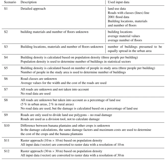
Scenario Description Used input data
S1 Detailed approach land use data
Roads with classes (lines) line 2001 flood data
Building locations, materials and number of floors
S2 building materials and number of floors unknown building locations
average material values average number of floors
S3 Building locations, materials and number of floors unknown number of buildings presumed to be
equally spread in the urban area
S4 Building density is calculated based on population density (three people per building) Population density is used to determine number of buildings in statistical sectors
S5 Building density is calculated based on number of people in study area (three people per building) Number of people in the study area is used to determine number of buildings
S6 Road classes are unknown
Average values for the width and the cost of the roads are used
S7 All roads are unknown and not taken into account
No road data are used
S8 All roads are unknown but taken into account as a percentage of land use (5 % in urban areas, 2 % in rural areas)
No road data are used, but the damage is calculated based on a percentage of land use
S9 Roads are only used to divide land use polygons – no road damage
Roads are used as a division tool, not to calculate damage
S10 Difference between banana plantains and other crops is unknown
In the damage calculations, the same damage factors and maximum costs are used to determine the cost of the crops and the banana plantains
S11 Raster approach (10 m×10 m) based on population density
All input data (vector) are converted to raster data with a resolution of 10 m
S12 Raster approach (30 m×30 m) based on population density
All input data (vector) are converted to raster data with a resolution of 30 m
The Japanese damage functions could be transferred to Ja-maica due to the similarities in geography and building engi-neering procedures. Most Japanese and Jamaican buildings are constructed in a similar manner with solid concrete or wooden walls. The distinction between these two building types is made in the damage functions as well as in the build-ing database of Annotto Bay. The calculated real damages were then summed up per land use polygon, in order to gen-erate a clear view of the building damage.
The damage to roads was calculated using the road net-work dataset (ODPEM, 2013a). This dataset divides the roads into four classes, each with their own properties, for example the width of the road. The line dataset was con-verted into polygons, based on the different widths. Using an average maximum road damage, calculated by Collier et al. (2013) for developing countries, and combining this with
damage factors from the Flemish LATIS flood risk assess-ment tool (Deckers et al., 2010), the real damage was then calculated for all roads.
dam-Table 3.Overview of the input data used per scenario.
S1 S2 S3 S4 S5 S6 S7 S8 S9 S10 S11 S12
Building locations X X X X X X X X X
Number of floors X X X X X X X X
Building material X X X X X X X X
Average building values X X X X X X X X X X X X
Critical buildings X X X X X X X X
Number of buildings X
Population density X
Number of people X
Roads X X X X X X X X X X
Road classes X X X X X X X X
Average road values X X X X X X X X X X
Land use data X X X X X X X X X X X X
Banana plants – crops X X X X X X X X X X X
Average crop values X X X X X X X X X X X X
2001 flood extent X X X X X X X X X X X X
Damage functions X X X X X X X X X X X X
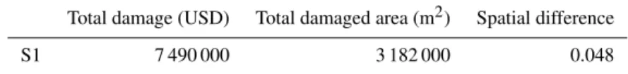
Table 4.Calculated total damage, total damaged area and spatial difference for S1.
Total damage (USD) Total damaged area (m2) Spatial difference
S1 7 490 000 3 182 000 0.048
age value was based on information from FAOSTAT (2014) and was multiplied with this damage factor to determine the crop damage cost. Since the damage factor for the banana plantains was 1, their real damage value was equal to the maximum damage value.
Since there is only very limited information on the exact consequences of the 2001 flood, the benchmark model could not be validated. However, the small amount of information that was available could serve as an indication. The number of affected houses, for example, was 749 (ODPEM, 2013a), while the benchmark model calculated this at 799. The over-estimation can be explained by the generalization done by the model, that does not take into account the fact that some houses will resist better than others and will thus have no damage. There were no comparable data for road and crop damage.
The lack of validation increased the uncertainty of the model. However, this research did not take into account the uncertainties of the input data or the model, since the aim of this research was to investigate the sensitivity of the model towards its input data. Hence, to identify the influence of each type of input data, S1 was an acceptable benchmark. 2.1.2 Results
The benchmark damage map visualizes the output of the flood risk assessment model for Annotto Bay, as shown in Fig. 4. Table 4 contains the three numeric elements on which the comparison of the scenarios is based: the total damage,
Figure 4.Scenario 1 (S1): benchmark damage map of Annotto Bay, using all available input data.
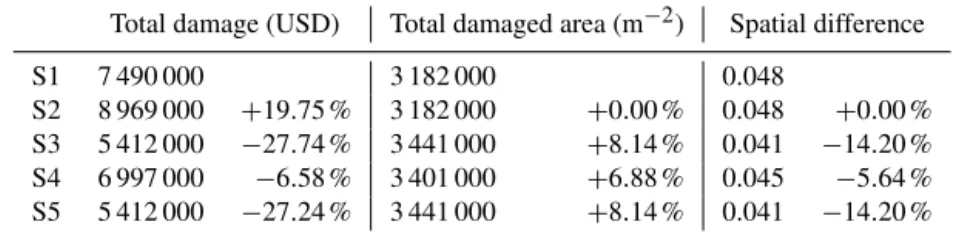
Table 5.Calculated total damage, total damaged area and spatial difference for S2, S3, S4 and S5 in comparison to S1.
Total damage (USD) Total damaged area (m−2) Spatial difference
S1 7 490 000 3 182 000 0.048
S2 8 969 000 +19.75 % 3 182 000 +0.00 % 0.048 +0.00 %
S3 5 412 000 −27.74 % 3 441 000 +8.14 % 0.041 −14.20 %
S4 6 997 000 −6.58 % 3 401 000 +6.88 % 0.045 −5.64 %
S5 5 412 000 −27.24 % 3 441 000 +8.14 % 0.041 −14.20 %
Table 6.Calculated total damage, total damaged area and spatial difference for S6, S7, S8 and S9 in comparison to S1.
Total damage (USD) Total damaged area (m2) Spatial difference
S1 7 490 000 3 182 000 0.048
S6 7 496 000 +0.08 % 3 180 000 −0.06 % 0.048 +0.00 %
S7 7 459 000 −0.41 % 3 171 000 −0.35 % 0.016 −66.18 %
S8 7 490 000 +0.00 % 4 347 000 +36.61 % 0.018 −63.47 %
S9 7 459 000 −0.41 % 3 159 000 −0.72 % 0.022 −54.91 %
2.2 Building damage sensitivity 2.2.1 Methods
In the next four scenarios, the sensitivity of the flood risk model towards the data used to calculate building damage was investigated. In S2, the information concerning materi-als and the number of floors was removed and replaced by average values for all buildings in Annotto Bay. In S3, the location of the buildings was also eliminated, leaving only the number of buildings in the total study area as informa-tion. In this scenario, after testing the available data in and around the study area, including the exact building locations and the land use data, 90 % of the buildings was presumed to be in urban areas and the other 10 % in rural areas. In S4 and S5, population information was used to determine the build-ing damage, based on the average number of three people per building (WRA, 2002). In S4, the population density per sta-tistical sector was used to calculate the number of buildings. In S5, however, only the total number of people in the study area was known. Here, the same assumption was made as in S3 about the division of buildings between rural and urban areas.
2.2.2 Results
Figure 5 shows the visual result of the four scenarios, while Table 5 shows the calculated damage, the damaged area and the spatial difference in comparison to the benchmark results of S1. Visually, no big changes can be observed in the indi-cation of the high-risk areas. The slightly lower spatial dif-ference in S3 and S5 does indicate a decrease in the level of detail. While S2 gives the result that is most similar to the result of S1, the table clearly shows an important differ-ence of 19.75 % in the calculation of the total damage cost.
This percentage rises to 20.88 % when only taking into ac-count the building damage. Although the visual result of S4 is less detailed than the benchmark, the spatial difference of 0.045 indicates a similar level of detail as in S1. Moreover, this scenario gives the best result towards the calculation of the total damage. The calculated building damage of S4 is USD 6.59 million, which is 6.96 % lower than the calculated building damage in S1.
2.3 Road damage sensitivity 2.3.1 Methods
Scenarios 6, 7, 8 and 9 were used to assess the sensitivity of the risk assessment towards the road data. In S6, the road classes were presumed to be unknown, giving all roads the same average width. S7 did not take the roads into account. In S8, the location of the roads was eliminated and, therefore, they were calculated as a percentage of the land use. After analyzing the available data in and around the study area, the percentages were set at 5 % roads in urban areas and 2 % in rural areas. S9 only used the road network to divide the land use polygons, but it did not take them into account in the damage calculations.
2.3.2 Results
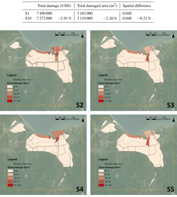
Table 7.Calculated total damage, total damaged area and spatial difference for S10 in comparison to S1.
Total damage (USD) Total damaged area (m2) Spatial difference
S1 7 490 000 3 182 000 0.048
S10 7 272 000 −2.91 % 3 110 000 −2.26 % 0.048 −0.21 %
Figure 5.Damage maps for Annotto Bay for S2, S3, S4 and S5. Top left: (S2) building materials and number of floors unknown; top right: (S3) building locations, materials and number of floors unknown; bottom left: (S4) building density is calculated based on population density; bottom right: (S5) building density is calculated based on number of people in study area.
There is a significant difference in damaged area between S1 and S8. Since the threshold value for road damage is 0 feet and the road damage is spread over the entire study area in S8, all flooded areas have damage. Moreover, visually, S8 shows a different, less accurate, result than the other scenar-ios, as shown in Fig. 6. The scenario has a low spatial dif-ference of 0.018. The total road damage cost of USD 32 000, however, is only 5.88 % lower than the damage cost in S1.
Although S7 clearly has a better visual result than S8, in-dicating the areas without any damage more accurately, the spatial difference of this scenario is lower. Due to a larger
Figure 6.Damage maps for Annotto Bay for S6, S7, S8 and S9. Top left: (S6) road classes are unknown; top right: (S7) all roads are unknown and not taken into account; bottom left: (S8) all roads are unknown but taken into account as a percentage of land use; bottom right: (S9) roads are only used to divide land use polygons – no road damage.
2.4 Crop damage sensitivity 2.4.1 Methods
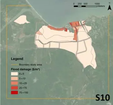
S10 tested the sensitivity of the model by assuming the dif-ference between banana plantains and other crops was un-known. An average maximum damage value was calculated from the values for banana plants and other crops, grown in Jamaica. The damage factor used was also an average, but only of the damage factors of other crops, since the damage factor for banana plants was 100 % for every water depth due to the duration of the flood.
2.4.2 Results
Since the real damage value of the crops is rather small in comparison to building damage values, S10 only has a small effect on the result. Therefore, the visual view of the map is almost identical to the benchmark damage map. This can be seen in Fig. 7. Furthermore, Table 7 demonstrates that the calculated total damage and damaged area differ only little from the values that were generated by the model used for S1. However, the crop damage cost of USD 154 000 in S10 is 58.60 % lower than the crop damage cost of USD 372 000 in S1.
2.5 Data type sensitivity 2.5.1 Methods
Table 8.Calculated total damage, total damaged area and spatial difference for S11 and S12 in comparison to S1.
Total damage (USD) Total damaged area (m2) Spatial difference
S1 7 490 000 3 182 000 0.048
S4 6 997 000 −6.58 % 3 401 000 +6.88 % 0.045 −5.64 %
S11 9 692 000 +29.40 % 3 807 000 +19.64 % 0.047 −1.67 %
S12 8 425 000 +12.48 % 3 613 000 +13.54 % 0.032 −33.61 %
Figure 7.Damage map for Annotto Bay for S10. (Difference be-tween banana plantains and other crops is unknown.)
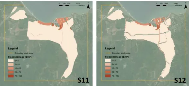
all input data were vector data. In areas with little data avail-able, however, a lot of information will have to be gath-ered from satellite imagery. Therefore, all input data in S11 and S12 were converted to raster data with a resolution of 10 m×10 m for S11 and 30 m×30 m for S12 to simulate satellite data. The former resolution was chosen since several commercial high-resolution satellite systems, e.g., SPOT, provide images with a world coverage with this resolution. The Landsat program uses the latter resolution and provides free images through an online service. The calculations for the building damage were based on population data, in the same way as in S4.
2.5.2 Results
Although the two damage maps, as shown in Fig. 8, visu-ally do not differ a lot from the maps of S1 and S4, Table 8 shows that the total damage cost is substantially higher than the cost in S1 and S4. All three separate damage costs show a large overestimation compared to S1 and S4. The road dam-age cost, especially, is 27 times larger in S11 and even 78 times larger in S12 than in S1. This is due to the fact that
road damage is calculated per pixel, and the pixels in both scenarios have a resolution larger than the width of the roads. Hence, the area assigned to roads is overestimated.
The total damaged area is also slightly larger due to the conversion of the polygon flood map to a raster map. Since the input of the scenarios was raster data, every pixel has been calculated separately. Therefore, the level of detail, and thus the spatial difference, is higher than in S7, S8 and S9. When comparing the results of S11 and S12, it can be stated that the spatial difference shows a growing decrease of accu-racy as the resolution of the raster data increases. Moreover, the visual result is less detailed and gaps arise in the final map.
3 Discussion
In all scenarios, more than 90 % of the total flood damage consists of building damages. Consequently, scenarios that test the models sensibility for building data show the largest deviations in the total damage. Figure 9 shows the deviation for every scenario from the total cost of S1.
When looking at the scenarios focussing on building dam-age, S4 has the best result, with a deviation of 6.58 % in re-lation to the result of S1. This scenario has calculated the damage cost based on population density per statistical sec-tor. In the case study of Annotto Bay, the benchmark study made use of the exact GPS locations of all buildings in the region. In many other areas in the SIDS, this detailed infor-mation is not available. Population data, however, exist for most regions free of charge. Since the model gives a good result, visually as well as in the total damage cost, this sce-nario must definitely be investigated further. The importance of an accurate average number of people per household was proven by running the same model with an average of two and an average of four people per household instead of the average of three, as given by WRA (2002). When testing the former, the total damage cost of USD 4.83 million is 35.55 % lower than S1, while the latter gives a resulting cost that is 21.75 % higher than the resulting damage cost of S1.
Figure 8.Damage maps for Annotto Bay for S11 and S12. Left: (S11) raster approach (10×10) based on population density. Right: (S12) raster approach (30×30) based on population density.
Figure 9.Deviation of total damage of all scenarios in relation to S1 (=0).
the land use is not a good simplification. Since buildings have a threshold value to be marked as “inundated” of 1,5 feet, but roads are marked immediately as flooded, the total damaged area in S8 is a big overestimation of the reality. This is af-firmed by the visual result, showing a lot of damaged area with a low cost per square meter.
Although S7 scores very well for the total damage as well as for the total damaged area, the result is a lot less accurate than the benchmark map. This becomes clear when looking at Fig. 11, which visualizes the deviation of the spatial dif-ference of all scenarios in relation to S1. In this figure, three scenarios that test the influence of road data have the high-est deviation and thus show significantly less detail in their damage map. Although the roads are negligible for the to-tal damage and the damaged area, they are, nonetheless, an indispensable part in creating a visually accurate map.
Visually, as well as in total damage and damaged area, the difference between crops and banana plantains has a small
effect on the results, as shown in Fig. 11. It must be stated that this is the case for this case study of Annotto Bay, where building damage is the major type of damage. When looking into other regions, where agriculture has a more important role, the difference between crops can be a lot more signifi-cant for the results. This has to be further investigated.
Figure 10.Deviation of total damaged area of all scenarios in relation to S1 (=0).
Figure 11.Deviation of spatial difference of all scenarios in relation to S1 (=0).
4 Conclusions
In industrialized countries, several risk-based flood tools were developed to predict and estimate the damages caused by inundations. Although a lot of detailed data are fed as input for these models, a certain degree of uncertainty is in-herent and can never be fully eliminated. However, such tools are constantly being optimized and are adopted for urban and rural planning in order to prevent damages from future inun-dations caused for instance by climate change or high de-grees of urbanization.
In developing countries the detailed data needed by these models are not available. Therefore, to determine whether the methodology used in the developed countries can be trans-ferred to developing countries, it is necessary know what the sensibility of the models is towards the input data.
For this research, a risk-based model inspired by the Flem-ish LATIS was used for the case study of Annotto Bay. The
results show that it is indeed possible to reduce the level of detail substantially, without adding significantly to the model uncertainties.
Since the 2001 flood especially hit the urban areas of An-notto Bay, the building data were the most significant type of data in this study. The scenario that uses the population density and the average number of people per household to calculate the number of buildings as a simplification for the exact location of the buildings produced the best results. The deviation of the total damage cost was only 7 % in compar-ison to the benchmark. As the population data are globally availability, in many cases for free, this is an important find-ing that can be transferred for case studies in other areas. It must be stated, however, that an accurate number of people per household is indispensable in this scenario.
dataset helps to divide the land use and determine the build-ing damage more precisely. In this light, the possibility of using remote sensing images to create road datasets must be investigated, since many available datasets do not include all roads. When using satellite imagery, the road classes can-not be taken into account, but this has been proven to have little impact on the result. Furthermore, a complete dataset can definitely help in defining building damage, since ev-ery building must have access to a road and will thus most likely be located close to this road. Combining this informa-tion with populainforma-tion data should be investigated further.
No conclusions could be made from the sensitivity analy-sis towards crop data, because, in this case study, the impact was too small. The results showed little difference between the benchmark scenario, where crops and banana plantains were treated separately, and the scenario where an average cost was used. To further investigate the impact of crop data, a more rural area should be investigated. However, it can al-ready be concluded that the difference between crops and ba-nana plantains can be eliminated in study areas where urban areas are most affected by flooding.
Finally, the data type plays an important role in the accu-racy of the final result of a risk assessment. Using raster data, from satellite imagery for example, causes an overestimation of the total damage and the damaged area due to the res-olution, which causes loss of information detail. Therefore, satellite imagery should always be vectorized before using it as input data in the risk methodology. In further research, more types of raster data with different resolutions should be tested, as well as combinations of raster and vector data.
This sensitivity analysis of the Annotto Bay flood model is a first and important step in determining which data are indispensable and which data can be adapted, replaced or ig-nored in a risk assessment. Although the road damage has a small impact on the overall damage cost, this data type is indispensable for an accurate visual result. Furthermore, it is shown that population density data, in combination with an average number of people in a household, are an adequate replacement of the exact housing locations as input data for building damage. Nonetheless, more research should be done in other regions to validate the results of the sensitivity anal-ysis and to investigate the impact to the damage types in dif-ferent situations.
5 Data availability
Most of the necessary input data for this research were gathered by ODPEM for the multi-hazard risk assessment performed in 2013 (ODPEM, 2013a). These data are not freely available and were only provided in the context of this research. Other input data can be found in Table 1, as well as the references to the data sources. The output damage map shapefiles for all scenarios can be consulted online (Glas et al., 2016).
Edited by: V. Kotroni
Reviewed by: two anonymous referees
References
Apel, H., Thieken, A. H., Merz, B., and Blöschl, G.: Flood risk assessment and associated uncertainty, Nat. Hazards Earth Syst. Sci., 4, 295–308, doi:10.5194/nhess-4-295-2004, 2004. Apel, H., Merz, B., and Thieken, A. H.: Quantification of
uncer-tainties in flood risk assessments, Int. J. River Basin Manage., 6, 149–162, doi:10.1080/15715124.2008.9635344, 2008.
Apel, H., Aronica, G. T., Kreibich, H., and Thiecken, A. H.: Flood risk analyses – How detailed do we need to be?, Nat Hazards, 49, 79–98, doi:10.1007/s11069-008-9277-8, 2009.
Carrington, C. D. and Bolger, M. P.: Uncertainty and
Risk Assessment, Hum. Ecol. Risk Assess., 4, 253–257, doi:10.1080/10807039891284325, 1998.
Collier, P., Kirchberger, M., and Söderbom, M.: The Cost of Road Infrastructure in Developing Countries, Oxford, Centre for the Study of African Economies, Department of Economics, 2013. Deckers, P., Kellens, W., Reyns, J., Vanneuville, W., and De Maeyer,
P.: A GIS for Flood Risk Management, in: Flanders, Geospatial Techniques in Urban Hazard and Disaster Analysis, chapt. 4, 51– 69, doi:10.1007/978-90-481-2238-7_4, 2010.
Dutta, D., Herath, S., and Musiake, K.: A mathematical model for flood loss estimation, J. Hydrol., 277, 24–49, doi:10.1016/S0022-1694(03)00084-2, 2003.
FAOSTAT: Food and Agriculture Organization of the United Na-tions: Statistics Division, Retrieved 21 January 2015 from foas-tat3.fao.org/download/Q/*/E:foastat3.fao.org/download/Q/*/E, 2014.
FEMA: HAZUS-MH MR4 Flood Model Technical Manual. Wash-ington DC: Federal Emergency Management Agency, Migitation Division, 2009.
Gall, M., Borden, K. A., Emrich, C. T., and Cutter, S. L.: The un-sustainable trend of natural hazard losses in the United States, Sustainability, 3, 2157–2181, doi:10.3390/su3112157, 2011. Glas, H., Jonckheere, M., De Maeyer, P., and Deruyter, G.: A
GIS-based flood risk tool for Jamaica: The first step towards a multi-hazard risk assessment in the Caribbean, 15th International Mul-tidisciplinary scientific geoconference SGEM 2015 Conference Proceedings, Albena, Bulgaria, STEF92 Technology Ltd, 2, 643– 650, doi:10.5593/SGEM2015/B22/S11.080, 2015.
Glas, H., Deruyter, G., De Maeyer, P., Mandal, A., and James-Williamson, S.: Analyzing the sensitivity of a flood risk assess-ment model towards its input data, Twelve Damage Scenarios, doi:10.5281/zenodo.182726, 2016.
Institute for Water Resources (IWR): Value to the nation: Flood risk management, Washington DC, USA, US Army Corps of Engi-neers, 2009.
ISDR: Global Assessment Report on Disaster Risk Reduction, Geneva, Switzerland, United Nations, 2009.
Kumar, R. and Acharya, P.: Flood hazard and risk assessment of 2014 floods in Kashmir Valley: a space-based multisensor ap-proach, Nat. Hazards, 84, 437–464, doi:10.1007/s11069-016-2428-4, 2016.
Kwak, Y., Shrestha, B. B., Yorozuya, A., and Sawano, H.: Rapid Damage Assessment of Rice Crop After Large-Scale Flood in the Cambodian Floodplain Using Tempo-ral Spatial Data, IEEE J. Sel. Top Appl., 8, 3700–3709, doi:10.1109/JSTAR.2015.2440439, 2015.
Merz, B., Kreibich, H., Thieken, A., and Schmidtke, R.: Assessment of economic flood damage, Nat. Hazards Earth Syst. Sci., 10, 153–163, doi:10.5194/nhess-10-1697-2010, 2004.
NLA: Landuse Jamaica. Kingston, Jamaica: The National Land Agency of Jamaica (NLA), 2001.
ODPEM: Damage Assessment Report, Kingston, Jamaica, Office of Disaster Preparedness and Emergency Management, 2001. ODPEM: Multi Hazard Risk Assessment Annotto Bay, St. Mary.
Kingston, ODPEM, 2013a.
ODPEM: National progress report on the implementation of the Hyogo Framework for Action (2011–2013), Kingston, Jamaica, Office of Disaster Preparedness and Emergency Management (ODPEM), 2013b.
Rajamannan, A. H.: Flood Protection for banana and plantain plants, Patent Application Publication, US20040242418 A1, 2004.
Statistical Institute of Jamaica: Census of population and housing 2011 Jamaica – General Report Volume I, Kingston, Jamaica, Statistical Institute of Jamaica, 2012.
UNESCO: Changing Small Island Developing States: A space per-spective on environmental change in the Caribbean, 2014. UNISDR: Making Development Sustainable: The Future of
Dis-aster Risk Management, Global Assessment Report on DisDis-aster Risk Reduction, Geneva, Switzerland, United Nations Office for Disaster Risk Reduction (UNISDR), 2015.
Vanneuville, W., Maeghe, K., De Maeyer, P., and Mostaert, F. : Spa-tial Calculation of flood damage assessment and risk ranking, AGILE 2005 8th Conference on Geographic Information Sci-ence, 549–556, 2005.
Weichel, T., Pappenberger, F., and Schulz, K.: Sensitivity and un-certainty in flood inundation modelling – concept of an analysis framework, Adv. Geosci., 11, 31–36, doi:10.5194/adgeo-11-31-2007, 2007.
WRA: Rapid Impact Assessment of Communities in Portland and St. Mary Affected by the October and November 2001 Flood Rains, Kingston, Water Resources Authority [WRA], 2002. Yu, J. J., Qin, X. S., and Larsen, O.: Joint Monte Carlo and