Improvisation Based on Imitating Human Players by
a Robotic Acoustic Musical Device
Kubilay K. Aydın, Aydan M. Erkmen, and Ismet Erkmen
Abstract – A new improvisation algorithm based on parameter estimation process for the imitation control of a robotic acoustic musical device “ROMI”, is presented in this paper. The musical state representation we have developed for controlling ROMI is a feature extractor for learning to imitate human players in a duet. ROMI’s intelligent control architecture also has the ability to provide player identification and performance training. In this paper we introduce the robotic device ROMI together with its control architecture, the musical state representation and focus on parameter estimation for imitation of duo players by ROMI. ROMI is aimed at jointly playing two instruments that belong to two different classes and improvises while assisting others in an orchestral performance.
Index Terms – State Representation, Improvisation, Musical Representation, Imitation, Control
I. INTRODUCTION
The objective in our work is to develop a robotic acoustic musical device that will be jointly playing at least two instruments while assisting others in an orchestral performance and also learn to imitate other players using the same instruments. This intelligence in imitation also provides player identification and performance training. In this study we introduce the robotic device together with its control architecture and focus on our musical state representation and automatic parameter estimation.
Building an all new acoustic musical instrument which plays itself by learning from human players and being capable of improvisation is the main focus of our research. In our work, instead of observing teachers who are experts in one acoustic musical instrument playing, we propose to observe groups of teachers playing instruments from two different musical groups namely strings and percussion.
Imitation of playing musical instruments and reproduction of acoustic music has been investigated in the well defined musical domain of jazz [1,2,3]. Research that focus on the presence of a single model which is always detectable in the scene and which is always performing the task that the observer is programmed to learn [4,5] has been made. Musical imitation have been handled in many studies, being facilitated through the use of computer generated music [6,7,8]. Various new electric musical instruments, including a wearable one and a PDA based one have been proposed [9,10,11]. A fixed-function mapping based imitation supporting system has also been proposed [12]. In our work, we concentrate upon imitating by ROMI to reproduce acoustic melodies from human teachers playing two types of instruments. In the next section, ROMI will be introduced together with its control architecture. In the third section, we will summarize our musical state representation that is used for controlling ROMI. The imitation process will be demonstrated by an example in the same section as well. Our proposed parameter estimation process will be presented and discussed in the fourth section. Section five concludes the paper.
II. DESIGN OF ROMI
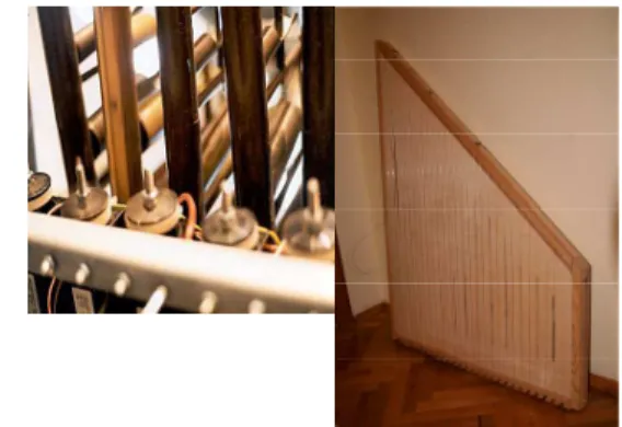
Two acoustic musical instruments from two different domains have been selected: Clavichord and Tubular bells in building ROMI where its main components are shown in Figure 1. ROMI utilizes a 2 octave string section with “note A” frequencies of 110 and 220 Hz and a tubular bells section having a 1 octave percussion with “note A” frequency of 55 Hz. The sound of the tubular bells section is not chromatic since the sound production properties of the copper tubes being used are very sensitive to temperature changes. Sound is generated by solenoids hitting the copper tubes and the harp strings as shown in Figure 1a. The string sections loudness is low compared to the tubes, so we utilize an amplifier for the string sections sound as shown in Figure 1b.
Sample sound recordings have been collected from two musicians playing a piano. These recordings are then utilized for the development of the imitation algorithms after they are converted to MIDI format by a commercial software. We developed a software converter which converts these MIDI representations, which are even incomprehensible to the human eye, into recognizable note sequences by ROMI enabling it to gain insight to the musical notes being played.
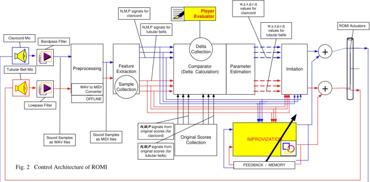
The control architecture of ROMI is given in Figure 2. Here two sets of musical signals are separately processed, one for the clavichord and the other process for tubular bells. The processing of these signals is never mixed in any of the application blocks. In learning mode, the human teachers play the respective musical instrument in an acoustically noise free environment. These sound samples are recorded by a microphone and further isolated from possible background noise by the application of a low pass filter for the tubular bells and a band pass filter for the clavichord and stored as a sound signal in WAV format. Then a commercial software is used to extract the musical notes in the sound signal, the result is an industrial standard file called MIDI where music is represented as note ON and OFF note commands. This process is shown in Figure 2 as “WAV to MIDI Conversion”. The MIDI file is then processed by our “Feature Extraction” stage and all recorded samples are stored in a “Sample Collection”. The feature extraction process converts the MIDI files into our “Musical State Representation” (MSR) that is
introduced in the next section. From this point, on all musical data is represented as three number streams N, M and P.
Original musical recordings representing models to be used for player identification and parameter estimation, are also converted into MSR and is stored in the “Original Scores Collection”. All data at these stages: the sample being processed, the Samples Collection being learned by ROMI in previous sessions and the Original Scores Collection are converted into our MSR format. The sample being processed is compared with the corresponding original score at the “Comparator” and a “Delta” vector is calculated as the distance of the sample from the original score. All delta vectors are stored in the “Delta Collection”, therefore the system not only stores the MSR for each sample but also stores the delta vector for each sample as well. This information is utilized by the “Parameter Estimation” process to estimate the six imitation parameters w, y, x, p, r, q. We are currently working on adding two applications to our system; Improvization and Player Evaluation. However, this paper pertains with the imitation stage where the outline of how imitation is achieved is explained in the next section. Sound is reproduced by ROMI and the reproduced sound is fedback to the system via microphones and control is achieved by minimizing the difference between the musical information stored in the MSR with the music generated.
III. MUSICAL STATE REPRESENTATION
In the “Musical State Representation” (MSR) that we have developed as a feature extractor for controlling ROMI, time (t) is slotted into 1/64th note duration. The maximum musical part length is set to 1 minute in our application for simplicity. This gives 1920 slots of time for each musical part (these numbers are based on the fact that the control algorithms are set for 120bpm). At the moment our MSR can work with a maximum of 256 different musical parts. Each musical part has a “Sample Collection” of maximum 128 samples performed by human teachers. MSR for each distinct sample “j” for a given musical part “g” (MPg) are stored at the “Feature Extraction” processes’ “Sample Collection” as shown in Figure 2. Our reason to chose a collection mode instead of a learning mode, where each new sample updates a
single consolidated data structure, is to keep all available variations alive for use in improvisation.
Each monophonic voice is represented by two number streams “N” and “M”, where the number values are whole numbers
between -127 and 128. “0” value for N and M and “-1”,”1”,
“-127” values for M streams have special meanings. Stream N
records the relative pitch difference between consecutive notes. Stream M records the relative loudness difference
between consecutive notes. The stream itself is a record of the duration of all notes. When there is a change in the current note, at least one of the two number streams register this event in the array structure by recording a non zero number. The number streams N and M consists of “0” values as long as
there is no change in the current note. Each number in these streams are equivalent to a 1/64th note duration. Note that for most people a 1/64th note is incomprehensibly short.
Silence is considered as a note with starting loudness value of -127. When silence ends the M stream resumes from the last
note loudness value attained before the silence.
If a note has the same note value as the previous note then the
N stream will record a “0” but the M stream will record the
loudness change value of “1” if loudness remains the same. Starting note value and velocity (loudness) is recorded for each musical part. ROMI’s cognition system is mostly focused upon duration, loudness and pitch difference taken in this order of importance.
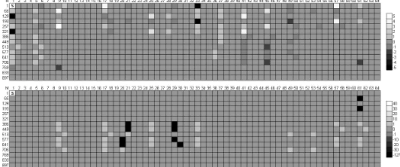
The following figures present a visualization of our MSR. Here the opening part of Lugwig von Beethoven`s Ecossais has been used as the sample. Figure 3, shows how the original recording is represented based on our MSR notation. Note that, the data is in fact a one dimensional array of whole numbers. To aid in visualization, this array has been continued from one line below for each 64 consecutive array elements. The numbers in the first row and column represent this arrangement. The first note is a special character which stores the information of its value and velocity. After the first note, all information is stored as the difference between two consecutive notes. As long as there are no note changes streams N and M consists of “0” values and are shown by mid
level gray tone in Figure3 & 4. As shown by the legend to the right of the figures.
+
Imitation
IMPROVIZATION
Feature Extraction Preprocessing
Clavicord Mic
Bandpass Filter
WAV to MIDI Converter Tubular Bell Mic
Lowpass Filter
Player Evaluator
ROMI Actuators
+
OFFLINE
FEEDBACK / MEMORY Comparator
(Delta Calculation)
Parameter Estimation Delta
Collection
Sound Samples as WAV files
Sound Samples as MIDI files
N,M,P signals for clavicord
N,M,P signals for tubular bells
N,M,P signals from original scores (for
clavicord) Sample
Collection
Original Scores Collection
N,M,P signals from original scores (for tubular bells)
w,y,x,p,r,q values for clavicord
w,y,x,p,r,q values for tubular bells
Lighter tones of gray indicate a positive change in N and M
streams; and darker tones of gray indicate a negative change. Therefore, every move from the mid level gray tone indicates a note change. Note that the changes in M streams has a larger
scale. Pure black array elements represent a “silence” in M
streams.
Figure 4, shows the MSR for one of the performances of the same musical part that ROMI “heard” by identifying one of our human teachers playing it on a piano. It is possible to “see” the difference with the original score where the “heard” recording from human teacher has small deviations from the original score.
Figure 5, shows the difference (Delta Vector) between the original score and the heard sample played on a piano by one human teacher. In the representation of the Delta Vector the value zero is shown with pure white color since the absolute value of the difference is of importance. In this figure all non zero array elements represent a note being played by the human teacher either with a wrong value or at the wrong time with respect to the original score. The number of non zero (non white) elements and their intensity is a measure of how good the performance of the human teacher was “heard”. This information can be used for parameter estimation and player evaluation as will be presented in the next section.
Number stream “P” is an event indicator similar to a token
state change in a Petri Net, where P values can assume any
rational number. The event indicator P number stream is
important in our improvisation algorithms. The addition of the event indicator P to the MSR has eased the detection of tempo
in musical parts. Using the MSR made of N, M and P streams,
ROMI imitates a musical piece based on the following algorithm. This algorithm uses six user defined parameters named as “w, y, x, p, r, q” which affect the reproduction quality of the imitated musical part.
1. Play all notes where Nij(t) has identical value with at least “w” percent of all j iterations, within a time window of p slots, with average value of all available non zero Mij(t) values
2. Play all notes, not already played by step 1, where Mij(t) has a loudness value in at least “y” percent of all j iterations, within a time window of r slots, with average value of all available Nij(t) values
3. Play all notes, not already played by step 1 or 2, where Pj(t) is not “0” for “x” percent of all available j iterations, within a time window of q slots, with average value of all available Nij(t) values and with average value of all available Mij(t) values
4. If Pj(t) lengths are different, select longest available length as music piece length with gradually decreased loudness, starting the decrease with the shortest available length
The imitation parameters and their effect to imitation performance are explained next:
w: This parameter is the main note generator. It uses the note change information, which is stored in the N streams. When a
sufficient number, “w” percent of all samples, have the same note change value within a time window of “p” slots, the imitation process executes a note change (plays a note) on ROMI. The effects of this parameter on imitation performance is discussed in the next section.
y: This parameter is the secondary note generator. It uses loudness change information, which is stored in the M streams
in the same mechanism as explained for “w”. A new time window parameter “r” had been defined other than “p” in order to gain more control on imitation performance.
x: This parameter is used for generating notes that are in the original score but were not produced by the note generators explained above. This parameter is used to track the changes in N and M streams and generate a note where there has been
sufficient changes in N and M streams to hint the existence of
a note. A new time window parameter “q” had been defined other than “p” and “r” in order to gain more control on imitation performance.
p: Due to slight tempo variations or less than perfect teacher performances, some notes are sounded about 1/64th of a note before or after they are in the original score. This parameter controls the width of a time window to group such note values together. The control unit places the note at the time slot where majority of the N values are situated. When there is a
draw, the first such slot is chosen.
r: Same as “p” but used for loudness variations. q: Same as “p” but used for event changes.
IV. PARAMETER ESTIMATION
Our proposed parameter estimation process incorporates an “Original Scores Collection” where each distinct musical part is in the form of our MSR. Therefore, each musical part has
Fig. 5 Delta in N & M Number Streams Between the Original Score and the Played Sample in MSR
N, M and P number streams in this collection. This original
recording is considered as the “nominal” MSR for a given musical part and the distance “Delta” for each recorded sample by human teachers can be evaluated.
If identity of each human teacher is known a priori for each sample, so it is possible to track the performances of each human musician if not this process becomes that of player identification.
Original score information for each musical part enables our proposed system to measure the “quality” of each imitated sample j, for a musical part that exists in the Original Scores Collection, the “nominal” sample, is assumed to have the highest “quality” if imitation mode is used but not during improvisation mode. The difference between the MSR of the nominal sample and the MSR of any given sample j yields difference “Delta Vector” for each recorded sample j. All delta vectors for known musical parts are stored in a separate “Delta Collection”.
The imitation process uses the six user defined parameters. Three of these parameters, w, y, x, define an averaging factor to be used in note reproduction by the imitation process of ROMI. The other three, p, r, q, define a time window in which this averaging function will be used. Changing these parameters effect the output quality.
The idea used to calculate Delta, can be used in a similar approach to estimate these user defined parameters controlling the imitation process. For each recorded sample set, collected from the same musician for a given part, modifying the w, y, x, p, r, q parameters to find a minimum for the associated Delta is possible. This is the output of the 3rd line in the algorithm above. Delta is not calculated for each separate sample but it is calculated for all the available samples by the same human teacher playing the same musical part.
At the end of test runs, the parameter estimation step showed us that there is no unique value set for minimizing the delta for these parameters but a range of parameter values has to be generated for very close Delta values. The test runs also showed that choices for p, q, r parameters are limited, since their value is in fact connected to the time granularity, or resolution, of the MSR. The w, y, x parameters can attain larger ranges. Due to the structure of the imitation process these parameters are not independent. The choice for one effects the plausible values for the others. For the test runs of the parameter estimation process, six samples for piano part Ecossais from Ludwig von Beethoven has been recorded by ROMI from two different human teachers.
The effects of different values for the imitation parameters are shown in the following figures. Each graph in these figures have been generated using the imitated piano parts musical reproduction, being compared with the original score. Some imitation parameters are set to fixed values to show the effects of changing others. Deltak values have been used for one of
the human teachers, total number of samples processed is six. Figures 6 and 7 show how Deltak values are effected by
changes in the main note generator parameters “y” and “w”. Parameters “y” and “w” effect the imitation performance in a similar way. Values below 20 for either parameter generate many notes that are not in the original score, resulting in high Deltak values. If either one of these parameters is kept around
70-90 the imitation performance is of acceptable quality. Note that, due to the nature of the calculation for Deltak values, it is
not possible to zero out the Deltak values.
x=55, p=3, r=3, q=4, j=1 to 6, k=1
100 120 140 160 180 200 220 240 260 280 300
10 20 30 40 50 60 70 80 90 100
y values
D
e
lt
a
k
w=10 w=20 w=30 w=40 w=50 w=60 w=70 w=80 w=90 w=100
x=55, p=3, r=3, q=4, j=1 to 6, k=1
100 120 140 160 180 200 220 240 260 280 300
10 20 30 40 50 60 70 80 90 100
w values
D
e
lt
a
k
y=10 y=20 y=30 y=40 y=50 y=60 y=70 y=80 y=90 y=100
The range of Deltak values are effected by the number of
samples processed with larger number of samples resulting in higher Deltak values. However this does not change the shape
of the given graphs with the local minimum still being achieved around 70-90 for these parameters. Values above 95 for either parameter generate less notes than the original score resulting in higher Deltak values.
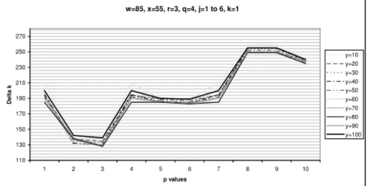
w=85, p=3, r=3, q=4, j=1 to 6, k=1
110 120 130 140 150 160 170 180
10 20 30 40 50 60 70 80 90 100
y values
D
elt
a k
x=10 x=20 x=30 x=40 x=50 x=60 x=70 x=80 x=90 x=100
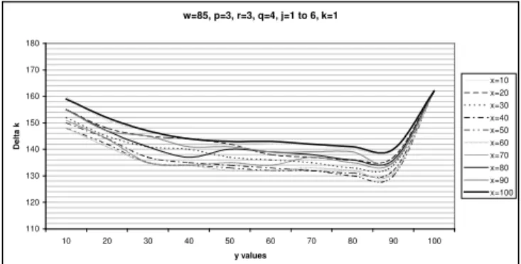
Figure 8 shows the effects of parameter “x” on imitation performance. This parameter has less impact on imitation performance compared to “w” and “y” parameters. This is understandable since the imitation algorithm generates notes based on N, M and P streams in this order. This results in
most of the notes already being produced by the N and M
streams with P stream having fewer opportunity to generate a
note and effect the imitation performance. For values below 25 this parameter generates notes that are not in the original score. For values above 95 it generates less notes than the original score. Figure 9 shows the effects of parameter “p”. Graphs for parameter “r” have the same shape and effect the imitation performance in a similar way as explained here for parameter “p”.
Fig. 6 Deltak for Varying y Values with 10 Different w Values
This parameter is used by the first note generator using N
streams and has the greatest impact on note production. The value 1 will produce less notes than the original score. Values 2 and 3 are optimal. Values above 3 produce more notes than the original score by combining two consecutive notes into one, increasing Deltak. The second jump in Deltak at “p” value
8 is due to the fact that more notes that is not in the original score are produced for every note shorter or equal to a quarter note within the time window defined by “p”. Even bigger jumps in Deltak should be expected for values 12 and 16 for
this parameter.
w=85, x=55, r=3, q=4, j=1 to 6, k=1
110 130 150 170 190 210 230 250 270
1 2 3 4 5 6 7 8 9 10
p values
D
elt
a k
y=10 y=20 y=30 y=40 y=50 y=60 y=70 y=80 y=90 y=100
V. IMPROVISATION BY RELAXATION OF IMITATION
PARAMETERS
In our studies we have seen that it is possible to use Improvisation by Relaxation of Imitation Parameters (IRIP) as a low level improvisation tool; whose parameters are defined within time intervals controlled by a higher level improvisation algorithm. This is an interesting subject that we are currently investigating. The initial results are presented in this section.
The values of imitation parameters that minimize Deltak
produce an output very similar to the original score, or the median of the samples. Improvisation can be achieve with limited success, by relaxation of the imitation parameters that result in non-minimum Deltak. Most of the imitation
parameters give higher Deltak if used below or above certain
values. However our tests showed that the values that produce less notes than the original score are less suitable for improvisation.
If imitation parameters are further relaxed the system tends to drift too much out of the original scores note frequency range. The resultant improvisation is more exiting due to higher variations but the overall musical part becomes fuzzy. We propose to use a partial application for the improvisation if the imitation parameters are further relaxed. For example, a mask as shown in Figure 10, can be applied. In this mask the white slots represent where the original score will be played back by the imitation algorithm and the black slots represent where the imitation parameters are very relaxed. For example the “black” slots set at y=50, w=50, x=50, p=2, r=2, q=3; and imitation parameters for the “white” slots set at y=85, w=85, x=55, p=3, r=3, q=4.
There can be many other choices for defining such a mask. For example, there can be masks with not only two sets of imitation parameter values (one for imitation and one for improvisation) but with more sets of varying values. Such an approach will add even more variations into the musical part. But then the obvious question is what controls the selection of such masks? The answer maybe “a higher level of improvisation algorithm”. There are some ground rules that we have discovered during test runs. These rules can be outlined as:
1. Short periods of IRIP does sound like a wrong note has been played. Therefore we suggest that the minimum duration for an IRIP part must be at least 1 seconds. 2. Long periods of IRIP tend to drift out of the scale of the
musical piece being played. This is due to our MSR. The most common result of the IRIP is the addition of the same note at a very close time interval of the original note. Since MSR is a difference representation, this addition of new notes in improvisation drift the note sequences out of the scale of the musical piece. This results the rest of the musical piece being played at a different pitch. To limit this effect, our proposition is that these intervals should not be larger than 2 seconds. And at certain intervals the musical piece should be returned to one absolute note value.
3. The starting time of an IRIP should be snapped to a grid of 1/8th note durations. This helps to ensure that the IRIP has the same tempo as the musical piece.
4. The duration of an IRIP should be multiples of 1/8th note durations. This helps to ensure that the IRIP has the same tempo as the musical piece.
5. If more than one IRIP is going to played in a musical piece. We advice to put imitation parts between IRIP parts, that are at least the same length of the last IRIP being played. This gives the listener the necessary clues at what the modal of the musical piece is.
The example in Figure 11 helps to visualize these ground rules. In this mask the white slots represent where the original score will be played back by the imitation algorithm and the black slots represent where the imitation parameters are very relaxed. The gray slots are where we recommend the start of an IRIP should be snapped to.
VI. CONCLUSION
Our studies for a higher level improvisation algorithm has two areas of investigation. One is to develop an improvisation algorithm based on n-grams including velocity information. The second one is to develop a patching algorithm which will analyze the current imitation and the generated improvisation and decide where to patch the improvisation. In this way our work will have a new approach to improvisation. Our current idea of how this patching could be implemented is to analyze the imitation and improvisation as a signal and match the
Fig. 9 Deltak for Varying p Values with 10 Different y Values
Fig. 10 Mask for Improvisation Intervals, Black Slots Represent Where Imitation Parameters are Very Relaxed
slopes of imitation and improvisation signals at the entry and exit points of the improvisation.
We experimented with our MSR to increase its performance in fast notes. The idea was to increase the time granularity of the system by defining a smaller time window; for example each time slot is a 1/128th note. However, if granularity of the discrete time model is increased, in order to pinpoint notes, the system shows a strong tendency to produce extra notes that were not intended. To limit this tendency p, r, q values can be increased, which effectively reduces the system to one with lower granularity.
Using the Delta Vector in Figure 5 is like ROMI listening to the “sound” of the Delta Vector for each wrong note. This leads to the possibility of user profiling by ROMI. In fact the data is readily available in the MSR of each sample to assess many aspects of the musician playing the musical part. Gathering this information was not a planned initial goal of this study. However, this is an important result that led to a valuable profiling by product.
REFERENCES
[1] K.K. Aydın, A. Erkmen, `Musical State Representation for Imitating Human Players by a Robotic Acoustic Musical Device`, IEEE International Conference on Mechatronics, 2011, to be published.
[2] R. Rafael, A. Hazan, E. Maestre and X. Serra. ‘A genetic rule-based model of expressive performance for jazz saxophone’, Computer Music Journal, Volume 32, Issue 1, p. 38-50, 2008.
[3] E. Cambouropoulos, T. Crawford and C. Iliopoulos, ‘Pattern Processing in Melodic Sequences: Challenges, Caveats &Prospects ’. Proceedings from the AISB ’99 Symposium on Musical Creativity , Edinburgh, Scotland,pp.42 –47, 1999.
[4] P. Gaussier, S. Moga, J. P. Banquet and M. Quoy. From perception-action loops to imitation processes: A bottom-up approach of learning by imitation. Applied Artificial Intelligence Journal, Special Issue on Socially Intelligent Agents. 12(7 8), pp. 701 729, 1998.
[5] Y. Kuniyoshi, M. Inaba and H. Inoue. Learning by watching: Extracting reusable task knowledge from visual observation of human performance. IEEE Transactions on Robotics and Automation, vol. 10, no. 6, pages 799 822, 1994.
[6] M. Goto, I. Hidaka, H. Matsumoto, Y. Kuroda, Y. Muraoka: A jam session system for interplay among all players. In: Proc. ICMC. Pp.346–349, 1996.
[7] Y. Aono, H. Katayose, S. Inokuchi: An improvisational accompaniment system observing performer’s musical gesture. In: Proc. ICMC. pp.106–107, 1995.
[8] M. Goto, R. Neyama: Open RemoteGIG: An open-to-the public distributed session system overcoming network latency. IPSJ Journal 43, pp.299–309, 2002.
[9] K. Nishimoto, et al.: Networked wearable musical instruments will bring a new musical culture. In: Proc. ISWC. pp.55–62, 2001. [10]T. Terada, M. Tsukamoto, S. Nishio: A portable electric bass using
two PDAs. In: Proc. IWEC. Kluwer Academic Publishers pp.286– 293, 2002.
[11]A. Yatsui, H. Katayose: An accommodating piano which augments intention of inexperienced players. In: Entertainment Computing: Technologies and Applications, pp.249–256, 2002.
[12]Gillic, K. Tang and R. Keller, ‘Learning Jazz Grammars’. Proceedings of the SMC 2009 - 6th Sound and Music Computing Conference, pp.125 –130, 2009.
Author Information
The authors are with Electrical and Electronics Engineering Department, Middle East Technical University, Ankara, Turkey