Analysis of 3D time-dependent acoustic problems via a generic BE substructuring algorithm based on iterative solvers

Analysis of 3D time-dependent acoustic problems via a generic BE

substructuring algorithm based on iterative solvers

F.C. Arau´jo*, D.R. Alberto, C. Dors

Department of Civil Engineering/UFOP, CEP 35400-000 Ouro Preto-MG, Brazil

Received 20 May 2002; revised 25 November 2002; accepted 27 November 2002

Abstract

In this paper, a generic BE/BE coupling algorithm based on iterative solvers is applied to solve 3D time-dependent acoustic problems. As regards the treatment of the time-dependence, a direct time-marching scheme is considered. Several types of boundary elements and cells are available in the code for the spatial description of the involved variables. Concerning the BE/BE coupling technique, its chief idea is to completely avoid storing and manipulating the zero blocks appearing in the coupled system by the use of iterative solvers. The global system matrix is not explicitly assembled; instead the algebraic subsystems (associated with the substructures of the model) are manipulated as they were independent of each other. An insight into the coupling strategy and the used iterative solver (Jacobi-preconditioned bi-conjugate gradient method) is given. Analyses of sound barriers are carried out for verifying the performance of the respective computational code modules.

q_{2003 Elsevier Ltd. All rights reserved.}

Keywords:3D Acoustics; Transient analyses; BE/BE coupling algorithms; Iterative schemes

1. Introduction

Sound waves take place when pressure disturbances propagate through a compressible fluid. Their investi-gation is necessary in a great many technical problems as, e.g. in the noise reduction near highways and in airports, prediction of sound fields in auditoria, noise control in industrial installations, design of vehicles, and several other situations associated with the comfort of human beings [1].

Important works concerning transient analyses in 2D acoustics by boundary element models were presented by Mansur and Brebbia [2,3] and Mansur [4]. After these first works, Dohner et al. [5], Meise [6], Antes [7], and Arau´jo et al. [8] published more advanced works related to 3D BE acoustic analyses in the time-domain. More recently, Antes and Baaran[9] applied the direct BEM to

analyze 3D noise radiation caused by independently moving surfaces. In this case, a time-domain BE formulation is indeed necessary. To describe the convective effects associated with the moving boundaries, they used the approach proposed by Gennaretti and Morino [10].

In this paper, the coupling strategy previously presented by Arau´jo et al. [11], which proved to be efficient for non-homogeneous frequency-dependent pro-blems, is applied to solve general 3D transient acoustic problems. As a boundary element formulation is involved, the procedure is quite suitable for analyzing exterior domain problems (infinite domains). On the other hand, the substructuring option (BE/BE coupling) is necessary for modeling thin elements, as, e.g. sound barriers, by means of direct standard BEM formulations.

To treat two-dimensional time-harmonic acoustic problems defined in unbounded different media, Cremers et al. [12] developed a special multi-domain BEM, in which infinite boundary elements are used to model boundaries and interfaces of infinite extent. Though not

0955-7997/03/$ - see front matterq2003 Elsevier Ltd. All rights reserved. doi:10.1016/S0955-7997(03)00021-3

www.elsevier.com/locate/enganabound

1 _{Tel.:þ55-21-2562-7196.}

* Corresponding author. Tel.:þ55-31-3559-1547; fax:þ 55-31-3559-1548.

necessary [13], this approach describes open domains more correctly. Other characteristic of the formulation presented by Cremers et al. [12] is that as a consequence of the chain assembly of the subdomains, i.e. subdomainj is coupled only with subdomains j2_{1 and} jþ1; the global non-symmetric matrix is banded. It is unfortunately not always possible to work with chain subdomain models, and, as a matter of fact, for modeling more general regions with use of substructures, more compli-cated sparse matrices are obtained as well. Optimized algorithms as, for instance, skyline and frontal ones are then necessary for solving efficiently the coupled system [14]. In this paper, the general and ideally optimized BE/ BE algorithm proposed in Ref. [11] is applied to solve time-domain acoustic problems.

As in the case of the design of sound barriers both thin elements and open domains are present, the algorithm proposed in this paper may be a very promising one. There are nowadays boundary element formulations based on the hypersingular integral equation, the so-called dual boundary element method, that has been successfully applied to simulate non-thickness bodies, as for instance sound barriers [15 – 18]. As a Cauchy principal value and a Hadamard finite part are present in the traction integral equation, special algorithms for their efficient evaluation [19,20] must be taken into account. An advantage of dual boundary element formulations is that no additional interfaces for modeling non-thickness barriers are necessary; this improves the precision of the results.

As regards the modeling of open domain with flat ground, efficient boundary element formulations based on the use of half-space Green’s functions[16,21,22]may also be derived; in this way one avoids discretizing the ground. In Ref.[23], Green’s functions that simulate the presence of tall buildings in the vicinity of sound barriers are also presented.

However, even in the cases above, in which dual BE formulations or Green’s functions for flat half-spaces are used, BE/BE coupling strategies may be inevitable; for instance, when non-homogeneous regions or large models have to be analyzed. In the latter case, substructuring techniques may be very useful for carrying out parallelized analyses.

In effect, substructuring strategies constitute a very important and general technique in computer mechanics, not exclusively restricted to BE formulations, but that considerably extend their range of applications. In previous works [14,24,25], either non-condensed or condensed strategies based on the use of direct solvers are reported.

To analyze real engineering problems, usually large, efficient procedures that reduce the storage area to a minimum and also be fast, must be idealized. In effect, these two topics are addressed in this paper, then iterative solvers make it possible to reduce the storage

area to a minimum, as the null coefficients of the sparse coupled system are not stored, and moreover may be much faster than the direct ones for large systems. Indeed, in the 90s, the iterative methods gained more and more acceptance in real-life industrial applications. Important recent books covering the use of iterative solvers in engineering were published by Axelsson [26], Hack-busch [27], and Saad [28]. In the particular case of BE systems of equations, successful applications of iterative methods have already been done by Mansur et al. [29], Barra et al.[30], Prasad et al. [31], Hribersek and Skerget [32], Leung and Walker [33], Skerget et al.

[34], and Valente and Pina [35]. In these works, Krylov

subspace methods that apply to general unsymmetric systems of equations are considered; mainly precondi-tioned versions of the BiCG, the GMRES, and hybrid BiCG methods, obtained by combining BiCG methods with other Krylov iterative methods [36], were incorpor-ated into BE algorithms. In this paper, the Jacobi-preconditioned BiCG is the only solver used in the BE/ BE coupling strategy.

As for linear transient analyses the system matrix remains unchanged during the whole analysis time, one may think that a LU-based direct solver should be the most attractive alternative. In fact, the matrix decompo-sition for a really large problem is a very hard computational task, so that iterative methods, even for linear transient problems, may be an interesting option. In this paper, one adopts as initial guess for calculating the current system solution that one of the last time step.

The analysis of sound barriers is considered for verifying the performance of the respective computer code modules. Important parameters for estimating the efficiency of the algorithms, as required CPU times, number of iterations, memory used, and response accuracy are discussed in the results of the paper.

2. Time-dependent boundary integral formulation

Small-amplitude sound waves are described by means of the linearized wave equation

u;ii2 1 c2

u;tt¼2gðx;tÞ; ð1Þ

where uðx;tÞ can be either the velocity potential or the acoustic pressure, and gðx;tÞ is a general volume source of acoustic energy [1,8]. Eq. (1) is to be solved under certain boundary conditions (prescribed acoustic pressure, velocity or acoustic impedance), and also under known initial values.

By using a general weighted residual statement[4]or by using Laplace transforms[8], Eq. (1), defined in a regionV

general boundary integral equation

cðjÞuðj;tÞ þð

G

ðt

0

pp_{ðx;t;j;tÞuðx;tÞdtdGðxÞ}

¼ð

G

ðt

0

up_{ðx;t;j;tÞpðx;tÞdtdGðxÞ}

þð

V

ðt

0

up_{ðx;t;j;tÞgðx;tÞdtdVðxÞ}

þc22ð

V

{v0ðxÞupðx;t;j;0Þ

þu0ðxÞu_pðx;t;j;0Þ}dVðxÞ; ð2Þ

whereup_andpp_{are, respectively, the fundamental solution}

and flux, given by

up_{ðx;t;j;0Þ ¼} 1

4prd t2 r c

; ð3Þ

ppðx;t;j;0Þ ¼2 1

4pr2 d t2 r c

þ r

c

_ d t2 r

c

_›r

›n; ð4Þ

and the integral free termcðjÞis calculated by

cðjÞ ¼1þlim

1!0 ð

G1

st_pp_{ðx;jÞdGðxÞ; ð5Þ}

st_pp_{ðx;jÞ representing the fundamental flux inG for}

time-independent potential problems. In Eq. (5),_G

1is a spherical

surface centered atj;introduced for evaluating the improper integrals[8], and cðjÞ corresponds exactly to the relation-ship

cðjÞ ¼ Fi

4p; ð6Þ

whereFiis the inner solid angle atj(Fig. 1).

Moreover, it should be noticed that the singular boundary integral in Eq. (2) associated withpp_{ðx;t;j;tÞexists only in}

the sense of the Cauchy principal value. In Arau´jo et al.[8],

a detailed derivation of the above boundary integral equation is provided.

In this paper, the description of the acoustic problem based on the excess acoustic pressure will be considered. One advantage of such a formulation is that the variables involved have physical meaning (pressures and particle velocities). Thus, as in the boundary integral formulation the function pðx;tÞ corresponds to normal derivatives of the acoustic pressure, this function does not directly represent the particle velocities. An additional transformation is needed to associate the normal derivative atx;pðx;tÞ;with the respective particle velocity. Namely, the following relationship, derived from the Euler’s equation[1], must be considered

pðx;tÞ ¼2r₀›vnðx;tÞ

›_t ; ð7Þ

where r₀ is the equilibrium density of the fluid, and vn denotes the velocity component of its particles normal to the boundaryGatðx;tÞ:

3. The time-dependent algebraic system

To derive the system of algebraic equations, the collocation method is used with respect to the space and time domains. Boundary elements are employed to approximate the boundary geometry and values, and integration cells, for evaluating the contributions of time-dependent volume sources and initial conditions. The approximation of the field variables along the time is carried out with usual time interpolation functions (Fig. 2). Thus, Eq. (2) can be transformed into a time-dependent system of algebraic equations, whose solution supplies the boundary unknowns u andp at the current time. Different types of boundary elements and integration cells are available in the computer code; namely, quadrangular and triangular, linear and quadratic boundary elements, and parallelepipedic linear and quadratic cells have already been implemented. Concerning the discretization of time-domain, a formulation that takes into account interpolation functions of a generic order (constant, linear, quadratic, etc.)

is provided below; yet the case of constant and linear time interpolation functions will be particularly emphasized.

To obtain the time-discretized version of Eq. (2), the initial conditions will be temporarily neglected, then they are actually not important for deriving the time-marching scheme. Thus, by generically approximatinguðx;tÞ;pðx;tÞ

andgðx;tÞwithin themth time step by

uðmÞðx;tÞ ¼ X

na

a¼1

Lð_amÞðtÞuaðmÞðxÞ; ð8Þ

pðmÞðx;tÞ ¼ X

nb

b¼1

M_bðmÞðtÞpbðmÞðxÞ; ð9Þ

gðmÞ_{ðx;tÞ ¼}X nz

z¼1

N_zðmÞðtÞgzðmÞ_{ðxÞ; ð} 10Þ

the following equation is found

cðjÞuðj;tnÞ þ Xn

m¼1 Xna

a¼1 ð

G

ðaÞ

Pnmðx;jÞuaðmÞðxÞdGðxÞ

¼ X

n

m¼1 Xnb

b¼1 ð

G

ðbÞ

Unmðx;jÞpbðmÞðxÞdGðxÞ

þX

n

m¼1 Xnz

z¼1 ð

V

ðzÞ

Unmðx;jÞgzðmÞðxÞdVðxÞ ð11Þ

with

ðaÞ

Pnmðx;jÞ ¼ð

tm

tm21

pp_ðx;t

n;j;tÞL ðmÞ

a ðtÞdt; ð12Þ

ðbÞ_Unm_{ðx;jÞ ¼}ðtm

tm21

up_ðx;t

n;j;tÞM ðmÞ

b ðtÞdt; ð13Þ

ðzÞ

Unmðx;jÞ ¼ð

tm

tm21

up_ðx;t

n;j;tÞN ðmÞ

z ðtÞdt: ð14Þ

In Eqs. (8) – (14), n indicates the current time point, n is the current time step, na; nb and nz are the number of

(time) points used for the time interpolation of uðx;tÞ;

pðx;tÞ and gðx;tÞ; respectively, uaðmÞ_{ðxÞ; p}bðmÞ_{ðxÞ and}

gzðmÞ_{ðxÞ denote the values of the respective functions at} the time points a; b and z of the mth time step, Lð_amÞðtÞ;

M_bðmÞðtÞ and N_zðmÞðtÞ are the adopted time interpolation functions, and the time integration limits in Eqs. (12) – (14) are given by

tm¼

mDt; ifm,n;

mDt; ifm¼n;

(

ð15Þ

where

m¼

m; ifna#2;

ðn2_{1Þ þ} ða21Þ ðna21Þ

; ifna$3; 8

> <

> :

ð16Þ

with a¼2;…na; na¼maxðna;nbÞ: Note that the

par-ameter a indicates the local order of the discrete time tn;

necessary to make possible the evaluation of the problem response at all time points of the current time step.

After considering the time translation property of the acoustic fundamental solution [8], the time-integrated kernels ðaÞPnm; ðbÞUnm; and ðzÞ_Unm

in Eqs. (12) – (14) can be reduced to integrations along the first time step only. Thus, at each time step, one has to calculate only the following time integrations

ðaÞ_PðnÞ_ðx;

jÞ ¼ð

m1Dt

0

pp_ðx;t

ðnÞ;j;tÞLaðtÞdt; ð17Þ

ðbÞ

UðnÞðx;jÞ ¼ð

m1Dt

0

up_ðx;t

ðnÞ;j;tÞMbðtÞdt; ð18Þ

ðzÞ

UðnÞðx;jÞ ¼ð

m1Dt

0

up_ðx;t

ðnÞ;j;tÞNzðtÞdt ð19Þ

with

m₁¼

1; ifna#2;

ða21Þ ðna21Þ

; ifna$3; 8

> <

> :

ð20Þ

a¼2;…;na; na¼maxðna;nbÞ: The time integrations in

Eqs. (17) – (19) are very simple and can be easily calculated in closed form. In Ref.[8], the results of the integrals in Eqs. (17) – (19) are furnished.

The above expressions are generic and may be used to obtain the system of algebraic equations associated with transient acoustic problems. Here, these expressions are however, particularized to the following time interpola-tions funcinterpola-tions: the potentials are linearly interpolated (na¼2 in Eq. (7)), the fluxes, constant- or linearly

(nb¼1 or nb¼2; respectively, in Eq. (8)), and the

volume sources, constantly interpolated (nz¼1 in Eq.

(9)). In this way, after the spatial discretization of the time-discretized boundary integral equation (11), one obtains

{Cþð2ÞHð1Þ}uðnÞ¼ð2ÞGð1ÞpðnÞþrðnÞ; ð21Þ

where

rðnÞ¼ð1ÞGðnÞpð0Þþ X

n21

m¼ni

{ð1ÞGðn2mÞþð2ÞGðn2mþ1Þ}pðmÞ

2 X

n21

m¼ni

{ð1ÞHðn2mÞþð2ÞHðn2mþ1Þ}uðmÞ

þ X

n21

m¼ni

Gðn2mþ1ÞgðmÞ ð22Þ

with

ni¼maxð1;n2nmaxþ1Þ; nmax¼ r_max

cDt þ2: ð23Þ

existence interval of the fundamental kernels given by

ðn2_1ÞcDt,r,ncDt [8].

In case of existing initial values to be considered, their contributions will be stored in an additional vector on the right-hand side of the system of Eq. (21), which will be dependent on only of the current time step. This vector will be determined in the most general cases with the use of integration cells.

4. The time-dependent BE/BE coupling

In order to develop the generic substructuring algor-ithm, the system of Eq. (21) is written for each subregion of the coupled system. The following systems are available

HkuðnÞ;k¼GkpðnÞ;kþrðnÞ;k; k¼1;ns; ð24Þ

where ns is the number of subregions of the model. By organizing the system of Eq. (24), so that one obtains on its left-hand side the unknown boundary values and the unknown interface potentials, and on its right-hand side the known boundary values and the unknown interface normal fluxes, it results:

Akb Hki

h i xð_bnÞ;k

uð_inÞ;k

8 < : 9 = ;

¼ Bk_b Gki

h i yð_bnÞ;k

pð_inÞ;k

8 < : 9 = ;

þrðnÞ;k; ð25Þ

where

Akb¼ HkbðuÞ 2G k bðpÞ

h i

; xð_bnÞ;k¼ u

ðnÞ;k b

pð_bnÞ;k

8 < : 9 = ;

; ð26aÞ

B_bk ¼ 2HkbðuÞ GkbðpÞ

h i

; yð_bnÞ;k¼ uð_bnÞ;k

pð_bnÞ;k

8 < : 9 = ;

: ð26bÞ

The subscripts above are defined as follows: bðuÞ defines the boundary part of the kth subregion with unknown potentials, bðpÞ that one with unknown fluxes, and i that one corresponding to the interface surfaces.bðuÞandbðpÞ

define, respectively, the boundary part with prescribed potential and normal flux.

As corresponding to the interface nodes of a given subregion k; both potentials and normal fluxes are unknowns, an additional number of equations will be necessary for making it possible to calculate all its unknown boundary values (including naturally its inter-face values). These equations are actually available in the equations of the other subdomains, so that if one assembles together the subsystems corresponding to all the substructures of the problem, a unique global system of equations with enough equations for determining the response of the problem in each subregion is obtained. In

explicit form, this system is given by

A1b 0 · · · 0 C11 C12 · · · C1s

0 A2b · · · 0 C21 C22 · · · C2s

. . . _. . . _. . . _. . . _. . . _. . . _. . . _. . .

0 0 · · · Ansb Cns1 Cns2 · · · Cnss 2 6 6 6 6 6 6 6 6 6 4 3 7 7 7 7 7 7 7 7 7 5

xð_bnÞ;1

xð_bnÞ;2

. . .

xð_bnÞ;ns

xð₁nÞ

xð₂nÞ

. . .

xðsnÞ 8 > > > > > > > > > > > > > > > > > > > > > > < > > > > > > > > > > > > > > > > > > > > > > : 9 > > > > > > > > > > > > > > > > > > > > > > = > > > > > > > > > > > > > > > > > > > > > > ; ¼ B1_b

B2_b

._. .

Bns_b~

2 6 6 6 6 6 6 6 6 6 4 3 7 7 7 7 7 7 7 7 7 5

yð_bnÞ;1

yð_bnÞ;2

. . .

yð_bnÞ;ns

8 > > > > > > > > < > > > > > > > > : 9 > > > > > > > > = > > > > > > > > ; þ rð_bnÞ;1

rð_bnÞ;2

. . .

rð_bnÞ;ns

8 > > > > > > > > < > > > > > > > > : 9 > > > > > > > > = > > > > > > > > ;

; ð27Þ

where n is the current time step, s is the number of interfaces, Ck

i denotes the coupling submatrix associated with the interface Gi and the kth subregion (containing terms of Hk_i and Gk_i), and x_iðnÞ;k and yðnÞ;k are the vectors containing the unknown and prescribed values at the nth time point, respectively. It should be noticed that the system (27) represents the most general form of a coupled system. Indeed, for most of the problems, some of the coupling matrices Cki are null; particularly when the subdomains are coupled in a chain way, like for instance finite element models for beams, the coupled system (27) reduces to a banded form [12]. In the algorithm proposed in this paper, the system (27) is actually not assembled; instead one works directly with the subsystems (25), as they were uncoupled. The use of iterative methods makes it possible to solve the system of Eq. (27) in an implicit way. To see how to do this, we first give the general expressions of the bi-conjugate gradient algorithm (BiCG method) [11].

Iterative formula:

xnþ1¼xnþlnpn: ð28Þ

Search directions:

pn¼ r

0

; ifn¼0;

rnþanpn

21_;

ifn$₁;

(

ð29Þ

p_pn

¼

p_r0 _¼r0_{; ifn¼0;}

p_rn

þanpp n21

; ifn$₁:

(

Residuals:

rn¼rn212ln21Ap n21_;

p_rn

¼p_rn21_2l

n21ATppn

21_:

ð31Þ

Parameters:

ln21¼

p_rn21;T_rn21

p_pn21;T_Apn21; an¼

p_rn;T_rn

p_rn21;T_rn21: ð32Þ

Two points are observed in the above iterative formulae: (1) the only operations necessary are multiplications matrix – vector and vector – vector; (2) the system matrix is not transformed during its resolution (as usual in iterative procedures). So, a special solution procedure can be developed to solve the system (27) in which the correspond-ing coupled system is not explicitly assembled. In effect, a loop over the number of all subregions is carried out and the contribution of each subregion, independently of each other, is taken into account in the operation considered (matrix – vector or vector – vector). Naturally, in suitable points of the solution algorithm (solver) the data of each subdomain are updated, so as to satisfy the coupling and, if necessary, also the flux continuity conditions at the interface nodes. At the

end, the final operation results of the current iteration are obtained by gathering the corresponding partial ones.

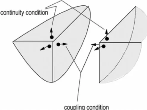
At nodes pertaining to interfaces between subregions i andj;i.e. ifx[Gij;the coupling conditions are given by

uiðx;tÞ ¼ujðx;tÞ

piðx;tÞ ¼2pjðx;tÞ

; ifniðxÞ ¼2njðxÞ;

(

ð33Þ

and the continuity ones, by

uiðx;tÞ ¼ujðx;tÞ

piðx;tÞ ¼pjðx;tÞ

; ifniðxÞ ¼njðxÞ:

(

ð34Þ

In Fig. 3, pairs of interface nodes are shown in which the

coupling and continuity conditions should be considered. In the computer code, a research is carried out in order to identify the interfaces (through their nodes) and then to introduce automatically the coupling and, if necessary, continuity conditions.

The interfaces between the subregions are defined by sets of coupled nodes, which are in turn defined based on the following criterion: coupled nodes pertain to two different domains, have the same co-ordinates, and opposite unit normal outward vectors. Associated with coupled nodes that have not the same geometrical position as those of other interfaces, that is, fornon-common interface nodes(Fig. 4), the respective number of equations is always enough, without any additional consideration on the interface variables, to calculate the potential and normal flux at them. In this case one will obtain, for each node, two equations for determining one potential and one flux. In case ofcommon interface nodes(Fig. 4), that is, if the coupled node is common to two or more interfaces, some additional considerations on the interface variables must be introduced in order to reduce the number of the corresponding unknowns; namely, flux continuity conditions must be taken into account (see Eq. (34) andFig. 3).

Fig. 3. Coupling and continuity conditions.

5. Applications

In order to observe the performance of the algorithm, the sound pressure distribution caused by an acoustic energy source, in the absence and presence of an infinite non-thickness barrier of heighth_b¼4:0 m;is analyzed (Fig. 5). The acoustic waves are radiated by a pulsating surface located at heighth_s¼1:5 m;and at distanced¼5:0 m from the barrier. The temporal variation of the normal component of the particle velocity is given by following pulses:

5.1. Sinusoidal pulse

In this case, the particle velocities are given by

vnðx;tÞ ¼v0sinðvtÞ: ð35Þ

The corresponding normal fluxes are

pðx;tÞ ¼2r₀v₀vcosðvtÞ: ð36Þ

For the analysis one considered v₀¼5:00 m=s and an excitation frequency corresponding to the octave-band center frequencyf ¼63 Hz:

5.2. Ricker’s pulse

Here, the speed of the particles and corresponding flux are expressed by (Fig. 6)

vnðx;tÞ ¼v0ð122t2Þe

2t2

; ð37Þ

Fig. 5. Infinite sound barrier.

Fig. 6. Ricker’s pulse.

pðx;tÞ ¼2r0v0

t0

ð4t32₆tÞe2t2; ð38Þ

where t¼ ðt2t_s=t₀Þ; t represents the time, t_s is the time point corresponding to the pulse amplitude, and pt₀; the dominant wavelet period[23]. A velocity amplitude ofv₀¼

5:00 m=s; and a dominant period of pt₀ ¼ ð1=63Þs were considered.

The source was tridimensionally simulated as a sphere of radius a¼0:05 m: As the dimensions of the source are much smaller than the length of the acoustic wave generated

ðl¼5:397 mÞ;the details of the pulsating surface will not indeed affect the sound being radiated.

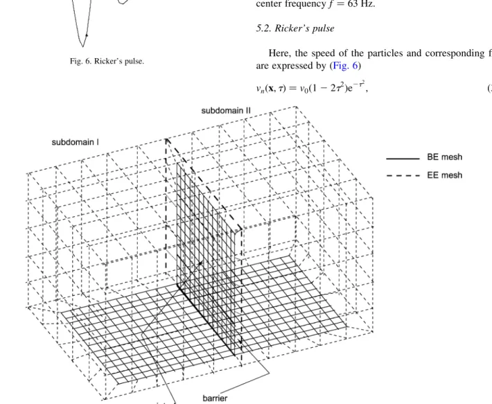
The boundary element mesh (Fig. 7) is generated so that the element sides be approximately 1=4 of the wavelength. Eight-noded (parabolic) boundary elements are adopted, and two subregions are considered to model the barrier. Additionally a mesh of enclosing elements is

used to make it possible to implicitly evaluate the principal values in the open subdomains. The BE mesh for subregion I has 1060 nodes and 320 elements, and for subregion II, 962 nodes and 288 elements. The respective EE meshes (of enclosing elements) for both

subdomains have 421 nodes and 130 elements. The source (spherical shell of radius a¼0:05 m) is modeled with 32 boundary elements; it is located in the subregion 1 and is not visible in Fig. 7. The physical constants of the considered medium (air) are:

c¼340:00 m=s ðsound speedÞ;

r0 ¼1:21 kg=m3 ðequilibrium densityÞ:

The adopted time step, Dt; is determined by observing the wave period T and the b coefficient, the latter being defined through

b¼ cDt

d ; ð39Þ

where d is the minimal diagonal of all elements of the BE mesh. The following criterion is adopted to choose the time step: it should not be too long compared with the wave period T; and the corresponding b coefficient, not so different from the unity. For the analyses here,

Dt¼1:5_£1023_{s was chosen, which corresponds} approximately to one-tenth of the wave period and to a

b¼0:27:

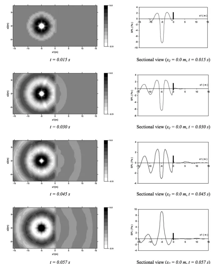
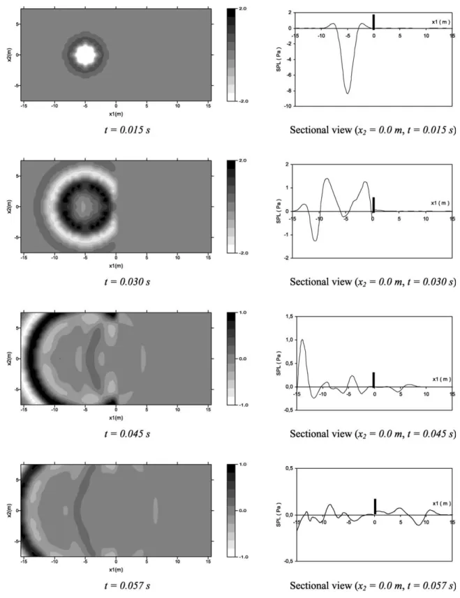
The results in terms of sound pressure level (SPL) are shown, for certain time points, in Figs. 8 and 9 for the sinusoidal pulse and the Ricker’s pulse, respectively. The sequence of snapshots in these figures displays the acoustic wave propagation in the presence of the barrier. The snapshots obtained in the absence of the barrier are not displayed.

The response in terms of insertion loss (IL) for both pulses is shown inFig. 10. The receiver points, at which the IL is calculated, are located behind the barrier at height h_r ¼1:5 m above the ground (Fig. 5), and the following

expression is used to evaluate the insertion loss (in dB)

ILðdBÞ ¼220logub

u_f ; ð40Þ

whereub anduf are the acoustic pressures in the presence and absence of the barrier, respectively.

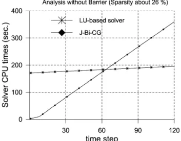
For the analyses carried out in this paper, the BE/BE coupling strategy based on the Jacobi-preconditioned biconjugate gradient solver was used[11]. To give an idea of the performance of this coupling strategy, the CPU times attained in the analysis are plotted against the sequence of time steps (Figs. 11 and 12). The direct solver considered for comparison is based on the non-symmetric LU decompo-sition and is non-optimized as regards the treatment of the matrix sparsity, which for the analyses here corresponds to approximately 26 and 32%, without and with barrier, respectively.

Fig. 10. Insertion loss curve.

Fig. 11. CPU time curve (without barrier).

The iterative scheme was stopped whenever krnþ1_k# tol; rnþ1 is the norm of the residual vector at the current iteration and tol¼1025_{;the adopted tolerance.}

The computer used for carrying out the analyses had an AMD ATHLON processor with 1.2 GHz and 768 Mbytes random access memory. The code was developed in FORTRAN and ran in a LINUX environment.

6. Conclusions

With the aid of the graphics inFigs. 8 and 9, which show the response in terms of SPL for both pulses considered, in the presence of an infinite barrier, the effectiveness attained by the barrier in reducing the noise in the acoustic shadow area ðx₁.₀:00 mÞ is visualized. Details of the time evolution of the wave propagation phenomenon, including superposition of incident and scattered waves, can also be observed.

More information on the barrier effectiveness can be taken from the insertion loss curves given inFig. 10. As one can see, the barrier is more effective for those points closer to it. The position of the receivers at which maximum efficiency is found can also be directly determined from the IL curves for both pulses.

The information related to the computational effec-tiveness of the algorithm is presented in Figs. 11 and 12, which show the CPU time values against the time steps. As expected, for the first time steps, the coupling strategy based on the iterative solver is much more effective than the LU-based one because the J-Bi-CG scheme is much faster than the LU-based solver. However, as a time-dependent linear problem is treated, the latter coupling algorithm begins to be more effective than the former when the number of time steps increases (after the 60th time step, see Figs. 11 and 12). Despite this (expected) fact, it should be noticed that the coupling strategy presented in this paper, which works directly with the subsystems and does not assemble the global matrix, may be a very interesting analysis tool for large industrial applications, mainly 3D ones. In such cases a LU decomposition may be a very hard computational task.

The frequency of the acoustic source studied is actually low; for higher frequencies the meshes must be suitably refined. Thus, the numerical effort for carrying out the time-domain analysis may increase considerably. Nevertheless, the strategy is general, and may be applied to any complex time-dependent problems described by the acoustic theory considered in his paper. Furthermore, the strategy is very suitable for developing parallelized computer codes. On the other hand, for non-linear time-dependent problems, the presented strategy is, for sure, quite convenient.

References

[1] Kinsler LE, Frey AR, Coppens AB, Sanders JV, Fundamentals of acoustics, New York: Wiley; 1982.

[2] Mansur WJ, Brebbia CA. Numerical implementation of the boundary element method for two-dimensional transient scalar wave propa-gation problems. Appl Math Modelling 1982;6:299 – 306.

[3] Mansur WJ, Brebbia CA. Formulation of the boundary element method for transient problems governed by the scalar wave equation. Appl Math Modelling 1982;6:307 – 11.

[4] Mansur WJ. A time-stepping technique to solve wave propagation problems using the boundary element method. PhD Thesis. South-ampton University, SouthSouth-ampton, England; 1983

[5] Dohner JL, Shoureski R, Bernhard RJ. Transient analysis of three dimensional wave propagation using the boundary element method. Int J Numer Meth Engng 1987;24:621 – 34.

[6] Meise T. BEM calculation of scalar wave propagation in 3-D frequency and time domain (in German). PhD Thesis. Fakulta¨t fu¨r Bauingenieurwesen, Ruhr-Universita¨t, Bochum, Germany; 1990 [7] Antes H. Applications in environmental noise. In: Ciskowiski RD,

Brebbia CA, editors. Boundary element methods in acoustics. New York: Computational Mechanics Publications; 1991. p. 225– 60. [8] Arau´jo FC, Mansur WJ, Carrer JAM. Time-domain three dimensional

analysis. In: Wu TW, editor. Boundary element acoustics. Funda-mentals and computer codes. London: Computational Mechanics Publications; 2000. p. 159– 216.

[9] Antes H, Baaran J. Noise radiation from moving surfaces. Engng Anal Bound Elem 2001;25:725– 40.

[10] Gennaretti M, Morino L. A boundary element method for the potential, compressible aerodynamics bodies in arbitrary motion. Aeronaut J R Aeronaut Soc 1992.

[11] Arau´jo FC, Martins CJ, Mansur WJ. An efficient BE iterative-solver-based sub-structuring algorithm for 3D time-harmonic problems in elastodynamics. Engng Anal Bound Elem 2001;25:795 – 803. [12] Cremers L, Fyfe KR, Sas P. A variable order infinite element for

multi-domain boundary element modeling of acoustic radiation and scattering. Appl Acoust 2000;59:185 – 220.

[13] Banerjee PK. The boundary element methods in engineering. London: McGraw-Hill; 1994.

[14] Bialecki RA, Merkel M, Mews H, Kuhn G. In- and out-of-core BEM equation solver with parallel and non-linear options. Int J Numer Meth Engng 1996;39:4215– 42.

[15] Krishnasamy G, Rizzo FJ, Liu Y. Boundary integral equations for thin bodies. Int J Numer Meth Engng 1994;37:107 – 21.

[16] de Lacerda LA, Wrobel LC, Mansur WJ. A dual boundary element formulation for sound propagation around barriers over an impedance plane. J Sound Vib 1997;202(2):235– 47.

[17] de Lacerda LA, Wrobel LC, Power H, Mansur WJ. A novel boundary integral formulation for three-dimensional analysis of thin acoustic barriers over an impedance plane. J Acoust Soc Am 1998;104(2):671 – 9. [18] de Lacerda LA, Wrobel LC, Power H, Silva JJR, Mansur WJ. Analysis of thin acoustic barriers using slender-body theory. Boundary elements in acoustics. Advances and applications, 1st ed. Southampton: Computational Mechanics Publications; 2000. [19] Rosen D, Cormack DE. The continuation approach for singular and

near singular integration. Engng Anal Bound Elem 1994;13:99 – 113. [20] Mantic V. On computing boundary limiting values of boundary integrals with strongly singular and hypersingular kernels in 3D BEM for elastostatics. Engng Anal Bound Elem 1994;13:115– 34. [21] Kawai T, Hidaka T, Nakajima T. Sound propagation above an

impedance boundary. J Sound Vib 1982;83:125– 38.

[22] Chandler-Wilde SN, Hothersall DC. Sound propagation above an inhomogeneous impedance plane. J Sound Vib 1985;98:475 – 91. [23] Godinho L, Anto´nio J, Tadeu A. Sound propagation around rigid

[24] Rigby RH, Alliabadi MH. Out-of-core solver for large, multi-zone boundary element matrices. Int J Numer Meth Engng 1995;38: 1507– 33.

[25] Ganguly S, Layton JB, Balakrishna C, Kane JH. A fully symmetric multi-zone Galerkin boundary element method. Int J Numer Meth Engng 1999;44:991 – 1009.

[26] Axelsson O. Iterative solution methods. New York: Cambridge University Press; 1994.

[27] Hackbusch W. Iterative solution of large linear systems of equations. New York: Springer; 1994.

[28] Saad Y. Iterative methods for sparse linear systems. New York: PWS Publishing; 1996.

[29] Mansur WJ, Arau´jo FC, Malaghini JEB. Solution of BEM systems of equations via iterative techniques. Int J Numer Meth Engng 1992;33: 1823– 41.

[30] Barra LPS, Coutinho ALGA, Telles JCF, Mansur WJ. Multi-level hierarchical pre-conditioners for boundary element systems. Engng Anal Bound Elem 1993;12:103– 9.

[31] Prasad KG, Kane JH, Keyes DE, Balakrishna C. Preconditioned Krylov solvers for BEA. Int J Numer Meth Engng 1994;37: 1651 – 72.

[32] Hribersek M, Skerget L. Iterative methods in solving Navier – Stokes equations by the boundary element method. Int J Numer Meth Engng 1996;39:115– 39.

[33] Leung CY, Walker SP. Iterative solution of large three-dimensional BEM elastostatic analyses using the GMRES technique. Int J Numer Meth Engng 1997;40:2227– 36.

[34] Skerget L, Hribersek M, Kuhn G. Computational fluid dynamics by boundary domain integral method. Int J Numer Meth Engng 1999;46: 1291 – 311.

[35] Valente FP, Pina HL. Iterative techniques for 3-D boundary element method systems of equations. Engng Anal Bound Elem 2001;25: 423 – 9.