Two-dimensional numerical investigations on the termination of bilinear flow in fractures

(1)

SED

5, 391–425, 2013

Two-dimensional numerical investigations

A. E. Ortiz R. et al.

Title Page

Abstract Introduction

Conclusions References

Tables Figures

◭ ◮

Back Close

Full Screen / Esc

Printer-friendly Version Interactive Discussion

Discussion

P

a

per

|

Dis

cussion

P

a

per

|

Discussion

P

a

per

|

Discussio

n

P

a

per

|

Solid Earth Discuss., 5, 391–425, 2013 www.solid-earth-discuss.net/5/391/2013/ doi:10.5194/sed-5-391-2013

Geoscientiic Geoscientiic

Open Access

Solid Earth

Discussions

This discussion paper is/has been under review for the journal Solid Earth (SE). Please refer to the corresponding final paper in SE if available.

Two-dimensional numerical investigations

on the termination of bilinear flow in

fractures

A. E. Ortiz R.1,*, R. Jung2, and J. Renner1 1

Institute for Geology, Mineralogy, and Geophysics, Ruhr-Universit ¨at Bochum, 44780 Bochum, Germany

2

JUNG-GEOTHERM, Gottfried-Buhr-Weg 19, 30916 Isernhagen, Germany

*

now at: Leibniz Institute for Applied Geophysics, 30655 Hanover, Germany

Received: 24 March 2013 – Accepted: 3 April 2013 – Published: 15 April 2013 Correspondence to: J. Renner (joerg.renner@rub.de)

(2)

SED

5, 391–425, 2013

Title Page

Tables Figures

◭ ◮

Back Close

Full Screen / Esc

Discussion

P

a

per

|

Dis

cussion

P

a

per

|

Discussion

P

a

per

|

Discussio

n

P

a

per

Abstract

Bilinear flow occurs when fluid is drained from a permeable matrix by producing it through an enclosed fracture of finite conductivity intersecting a well along its axis. The terminology reflects the combination of two approximately linear flow regimes, one in the matrix with flow essentially perpendicular to the fracture and one along the fracture

5

itself associated with the non-negligible pressure drop in it. We investigated the charac-teristics, in particular the termination, of bilinear flow by numerical modeling allowing an examination of the entire flow field without prescribing the flow geometry in the matrix. Fracture storage capacity was neglected relying on previous findings that bilinear flow is associated with a quasi-steady flow in the fracture. Numerical results were

general-10

ized by dimensionless presentation. Definition of a dimensionless time that other than in previous approaches does not use geometrical parameters of the fracture permitted identifying the dimensionless well pressure for the infinitely long fracture as the master curve for type curves of all fractures with finite length from the beginning of bilinear flow up to fully developed radial flow. In log-log-scale the master curve’s logarithmic

15

derivative initially follows a 1/4-slope-straight line (characteristic for bilinear flow) and gradually bends into a horizontal line (characteristic for radial flow) for long times. Dur-ing the bilinear flow period, isobars normalized to well pressure propagate with fourth and second root of time in fracture and matrix, respectively. The width-to-length ratio of the pressure field increases proportional to the fourth root of time during the bilinear

pe-20

riod and starts to deviate from this relation close to the deviation of well pressure and its derivative from their fourth-root-of-time relations. At this time, isobars are already significantly inclined with respect to the fracture. The type curves of finite fractures all deviate counterclockwise from the master curve instead of clockwise or counterclock-wise from the 1/4-slope-straight line as previously proposed. The counterclockwise

25

(3)

SED

5, 391–425, 2013

Title Page

Tables Figures

◭ ◮

Back Close

Full Screen / Esc

Discussion

P

a

per

|

Dis

cussion

P

a

per

|

Discussion

P

a

per

|

Discussio

n

P

a

per

|

fracture conductivities TD<1, a significant pressure increase is not observed at the

fracture tip until bilinear flow is succeeded by radial flow at a fixed dimensionless time. For TD>10, the pressure at the fracture tip has reached substantial fractions of the

associated change in well pressure when the flow field transforms towards intermittent formation linear flow at times that scale inversely with the fourth power of

dimension-5

less fracture conductivity. Our results suggest that semi-log plots of normalized well pressure provide a means for the determination of hydraulic parameters of fracture and matrix after shorter test duration than for conventional analysis.

1 Introduction

Transient fluid flow in fractures or faults plays an important role for the production of

10

oil and gas, for fresh water supply and the production of geothermal energy especially from artificial fracture systems, so called Hot-Dry-Rock (HDR) or Enhanced Geother-mal Systems (EGS). Flow in fractures and fracture networks may as well be important for the triggering of seismicity by precipitation (e.g. Hainzl et al., 2006), by groundwater recharge (e.g. Saar and Manga, 2003), by hydraulic stimulation (e.g. Deichmann and

15

Ernst, 2009; Majer et al., 2007; Shapiro and Dinske, 2009), and by water level changes in dams (e.g. Chen and Talwani, 1998).

For fractures in an impermeable rock matrix, fluid flow and pressure propagation are restricted to the fracture volume and are thus exclusively controlled by the hydraulic dif-fusivity of the fractures. In contrast, fluid flow and pressure propagation in fractures is

20

accompanied by fluid exchange with a permeable rock matrix, a rather complex prob-lem for mathematical treatment. A first analytical solution was presented in the context of well testing (Cinco-Ley et al., 1978) that applies to the case of fluid production from boreholes subsequent to hydraulic fracturing. Cinco-Ley et al. (1978) simplified the flow field as a superposition of two fields of parallel flow, one in the fracture and one in

25

(4)

SED

5, 391–425, 2013

Title Page

Tables Figures

◭ ◮

Back Close

Full Screen / Esc

Discussion

P

a

per

|

Dis

cussion

P

a

per

|

Discussion

P

a

per

|

Discussio

n

P

a

per

1981). Evidence for bilinear flow was reported from hydraulic tests after hydraulically fracturing a low permeable matrix, e.g. in tight basins that produce gas (Rushing et al., 2005; Stright and Gordon, 1983) and in sedimentary and granitic geothermal reser-voirs (H ¨aring et al., 2008; Jung and Weidler, 2000; Ortiz et al., 2011; Zimmermann, 2006). Interest in unconventional gas recovery from tight formations triggered studies

5

considering horizontal wells, too (see for example Du and Stewart, 1995; Jelmert and Vik, 1995; Verga and Beretta, 2001).

For constant production, a bilinear flow field is accompanied by a decrease of the wellbore pressure proportional to the fourth root of elapsed pumping time. The time window, during which this fourth-root relation can be observed, is however finite and

10

thus long term predictions – of great practical importance for exploitation of liquid or gaseous resources – are erroneous when using this relationship. Therefore, constrain-ing estimates of the end time of bilinear flow received attention in previous research (Cinco-Ley and Samaniego-V., 1981; Weir, 1999). Since radial flow dominated by the matrix properties develops when this time is exceeded it specifically marks the end of

15

the gain due to a stimulation operation involving hydraulic fracturing.

Until today, the physical understanding of the proposed relations for the end time of bilinear flow is incomplete. In this study, we rely on numerical simulations using a two dimensional finite element model in order to investigate the hydraulic diffusion in finite conductivity fractures. We include an analysis of the spatio-temporal characteristics of

20

the entire pressure field in fracture and matrix in order to clarify the flow processes that lead to the termination of bilinear flow and to substantiate quantitative rules for the end of bilinear flow. Outlining the end time and investigating the pressure field in a dimensionless parameter space allow us to generalize our findings obtained for specific cases to fractures with a range of dimensionless fracture conductivities. Focus is put

25

(5)

SED

5, 391–425, 2013

Title Page

Tables Figures

◭ ◮

Back Close

Full Screen / Esc

Discussion

P

a

per

|

Dis

cussion

P

a

per

|

Discussion

P

a

per

|

Discussio

n

P

a

per

|

formulation, describe the chosen modeling approach, report results and subsequently discuss them in the light of their practical use.

2 Background and approach

2.1 Governing equations for the hydraulics of a fractured well

For a well intersected by a single fracture and surrounded by a permeable matrix, two

5

basic hydraulic equations, partial differential equations for fluid pressurep, have to be considered, namely

∂p

∂t =Dm∇

2_p ₍₁₎

for flow in the infinite, isotropic and homogeneous matrix and

∂p

∂t =DF∇ 2_p

+qF(t)

hSF

(2)

10

for flow in the fracture. The two equations are coupled by the fluid flow between ma-trix and fracture,qF(t) (see for example Cinco-Ley et al., 1978). Here, Dm=km/ηfsm

andDF=TF/ηfSFdenote the hydraulic diffusivity of the matrix (m) and the fracture (F),

respectively, comprising matrix permeability km and specific storage capacity of the

matrixs_m, fluid viscosityη_f, fracture conductivityT_F=k_Fb_F(product of fracture

perme-15

abilitykF and fracture width bF) and fracture storativity SF=sfbF (product of specific

storage capacity of fracturesF and fracture widthbF).

Specific solutions of the governing Eqs. (1) and (2) for particular initial and boundary conditions have led to the distinction of characteristic flow regimes.Radial flow, charac-terized by a well pressure changing proportionally to the logarithm of elapsed pumping

20

(6)

SED

5, 391–425, 2013

Title Page

Tables Figures

◭ ◮

Back Close

Full Screen / Esc

Discussion

P

a

per

|

Dis

cussion

P

a

per

|

Discussion

P

a

per

|

Discussio

n

P

a

per

well. For homogeneous and isotropic media, diffusion of pressure perturbations obeys a linear scaling relation between the square of the characteristic propagation distance

Lc and the characteristic propagation time tc involving the hydraulic diffusivity of the

matrix, i.e.D_m_∼L2c/tc (see for example radius of investigation or drainage in Bourdet,

2002; Chaudhry, 2004; Dake, 2001; Earlougher, 1977; Horne, 1995; Matthews and

5

Russell, 1967). Highly permeable fractures, i.e. fractures in which the pressure gradi-ent is negligible, intercepting the well may extend the effective production surface such that flow in the subsurface is actually directed towards this extended surface rather than radial towards the well (e.g. Jenkins and Prentice, 1982). Such flow geometry is termed formation linear flow since straight flow lines are thought to result in the

ma-10

trix. The well pressure changes proportionally to the square root of elapsed pumping time. Thebilinear flow regime is encountered when the flow is approximately linear in both the fracture or narrow zone of high conductivity and the matrix (e.g. Butler and Liu, 1991). In this regime the finite conductivity of the fracture leads to a finite pressure gradient in the fracture (Boonstra and Boehmer, 1986; Gringarten, 1985). Fractures in

15

an impermeable matrix result infracture linear flow, per-se indistinguishable from for-mation linear flow regarding the power law relation between well pressure and elapsed pumping time.

2.2 Modeling approach

In our study, we focus on fractures with negligible storage capacity SF→0, i.e. the

20

fracture is considered undeformable and the amount of fluid in the fracture is consid-ered small enough for its compressibility to be neglected. In this approximation, Eq. (2) reads

0₌TF

η∇ 2_p

+qF(t)

h , (3)

i.e. the pressure in the fracture obeys an inhomogeneous diffusion equation with a

25

(7)

SED

5, 391–425, 2013

Title Page

Tables Figures

◭ ◮

Back Close

Full Screen / Esc

Discussion

P

a

per

|

Dis

cussion

P

a

per

|

Discussion

P

a

per

|

Discussio

n

P

a

per

|

pressure with time are considered to be dominated by the fluid transfer between matrix and fracture. Previous studies revealed that only for small dimensionless times the flow in the well and the flow in the matrix deviate from each other due to storage effects in the fracture (e.g. Weir, 1999). In the classical dimensionless form of Eq. (2) (see Eq. A-1 in Cinco-Ley and Samaniego-V., A-198A-1), the transient term on the left side appears

5

multiplied by the diffusivity ratioκ=Dm/DF. When this ratio is small, the effect of the

intrinsic transient term on wellbore pressure becomes important only for extremely small values of time and thus can be neglected for bilinear flow (see Cinco-Ley and Samaniego-V., 1981; Riley, 1991).

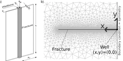
We use a two dimensional finite element model consisting of a fracture with half

10

lengthxF positioned on thex-axis (aty=0, see Fig. 1a) and intercepting a well along

its axis. Flow in the fracture of finite conductivity embedded in the permeable matrix is approximated as one-dimensional and wellbore storage is neglected. Thus, Eqs. (1) and (3) are implemented as

∂p ∂t =Dm

∂2p ∂x2+

∂2p ∂y2

!

(4)

15

and

TF ηf

∂2p ∂x2+

qF(x,t)

h =0. (5)

The origin of the coordinate system coincides with the well, actually represented by a point source with a flow rateqw/hdetermined from the true flow rate in the wellqwand

the height of the open well sectionh(Fig. 1). The fluid flow between matrix and fracture

20

qF(x,t)=2 km

ηf ∂p ∂y

y=0

(8)

SED

5, 391–425, 2013

Title Page

Tables Figures

◭ ◮

Back Close

Full Screen / Esc

Discussion

P

a

per

|

Dis

cussion

P

a

per

|

Discussion

P

a

per

|

Discussio

n

P

a

per

couples the two equations where the factor of 2 accounts for the communication via the two fracture surfaces.

In principle, numerical analysis does not require to prescribe the flow geometry in the matrix as do the majority of previously presented analytical solutions. The assumption of most analytical treatments, that flow lines in the fracture and in the matrix remain

5

strictly perpendicular to each other, indeed cannot hold towards the end of bilinear flow. The pressure di_ffusion in the matrix proceeds proportional tot1/2 ultimately sur-passing pressure diffusion in the finite conductivity fracture that scales witht1/4. Thus, eventually isobars have to change direction with increasing time.

We performed more than 30 simulations. In order to ensure the occurrence of

bilin-10

ear flow, fracture length was varied from 1.5 to 1500 m, while the further parameters remained constant (qw/h=2×10−

4

m2s−1, ηf=2.5×10− 4

Pa s, TF=1.5×10− 16

m3,

km=1×10− 18

m2, andsm=1×10− 11

Pa−1). An effect of the model boundaries on the simulation results was avoided by locating them far from the fracture (about 600 to 1200 m).

15

2.3 Dimensionless formulation

Our numerical modeling is performed with dimensional properties but for reporting re-sults we use non-dimensional parameters in order to foster a fundamental understand-ing of bilinear flow in our conceptual study. Previous analyses of flow regimes employed a variety of non-dimensionalization approaches. Here, we use the conventional

defi-20

nition for dimensionless pressure (see for example Earlougher, 1977; Matthews and Russell, 1967)

pwD=2π k_mh qwηf∆

(9)

SED

5, 391–425, 2013

Title Page

Tables Figures

◭ ◮

Back Close

Full Screen / Esc

Discussion

P

a

per

|

Dis

cussion

P

a

per

|

Discussion

P

a

per

|

Discussio

n

P

a

per

|

However, we use a modified definition of dimensionless time

τ=tD

T_D2 = Dmk

2 m

T_F2 t (8)

wheretD=tDm/x 2

Fis the classical definition of dimensionless time for an infinite

reser-voir adapted for the flow in fractures by replacing radial distance r with half-fracture length xF (Cinco-Ley et al., 1978; Earlougher, 1977; Matthews and Russell, 1967).

5

Furthermore, the dimensionless fracture conductivity is defined by

TD= T_F kmxF

. (9)

The employed model parameters correspond to values ofTDranging from 0.1 to 100.

Our choice of non-dimensional parameters is guided by the necessity to avoid frac-ture storage capacity and the request to also avoid fracfrac-ture length. When fracfrac-ture

10

length is used as an explicit parameter in the conventional definition of dimensionless time, one encounters the problem that “time” becomes ill defined for very long or in-finitely long fractures. The formulation should however be apt for fractures with a range of finite lengths, such as created for example during hydraulic fracturing operations, as well as for fractures with “infinite” length, such as encountered when length simply

15

exceeds the influence zone of the pumping operation. The latter situation may rather be typical for stimulations in a geothermal context that create a connection between the well and either an extended network of natural fractures or a large geological fault.

2.4 Previously presented solutions for bilinear flow

The theoretical background of bilinear flow was first presented by Cinco-Ley

20

(10)

SED

5, 391–425, 2013

Title Page

Tables Figures

◭ ◮

Back Close

Full Screen / Esc

Discussion

P

a

per

|

Dis

cussion

P

a

per

|

Discussion

P

a

per

|

Discussio

n

P

a

per

at constant flow rate is proportional to the fourth root of time in the bilinear flow regime. This result, subsequently confirmed by several approaches (e.g. Riley, 1991) reads

pwD= π

Γ 5/4√

2τ

1/4

≃2.45τ1/4 (10)

for the dimensional well pressure during bilinear flow with our set of non-dimensional parameters. Thus, we get a unique relation between non-non-dimensional well

5

pressure and non-dimensional time independent of any further model parameters. Some approximate analytical solutions for the pressure distribution in infinitely long fractures were derived in previous studies (see Boonstra and Boehmer, 1986; Weir, 1999). Notably, Boonstra and Boehmer (1986) already demonstrated that during a cer-tain sequence of bilinear flow the pressure distribution is governed by a single variable

10

combining time and distance (w in their notation). Weir (1999) subsequently empha-sized the self-similarity of the pressure function withx4/tin contrast to Theis’ solution for a homogeneous reservoir (also called line source or exponential-integral solution, Earlougher, 1977; Matthews and Russell, 1967; Theis, 1935) that admits r2/t as a self-similar variable.

15

In their seminal study, Cinco-Ley and Samaniego-V. (1981) report three expressions for the end time of bilinear flow but did not explicitly state how these relations were derived. Essentially, two extended regimes separated by a short intermediate regime are found for end time as a function of dimensionless fracture conductivity.

3 Results

20

(11)

SED

5, 391–425, 2013

Title Page

Tables Figures

◭ ◮

Back Close

Full Screen / Esc

Discussion

P

a

per

|

Dis

cussion

P

a

per

|

Discussion

P

a

per

|

Discussio

n

P

a

per

|

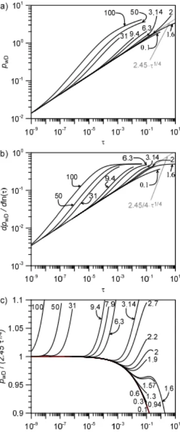
3.1 Evolution of the well pressure

Following common praxis, results are presented in the form of type curves (in log-log scale) of the dimensionless well pressure and its dimensionless logarithmic derivative versus dimensionless time (Fig. 2a, b). The main features can be best explained using the derivative (Fig. 2b). Characteristic for bilinear flow, the derivatives follow a straight

5

line with slope 1/4 over a certain period of dimensionless time. For sufficiently high dimensionless fracture conductivities (i.e. TD≫1), the derivative first turns

counter-clockwise into a straight line with slope 1/2 corresponding to formation linear flow, fully developed only for TD>50 (Fig. 2b). Ultimately, derivatives bend into a unique

hori-zontal line (dpwD/d lnτ=0.5) for all fracture conductivities indicating that radial flow is

10

reached. The dimensionless time to reach fully developed radial flow increases with decreasingTDand is highest forTD=0.

The log-log plots of the well pressure and its derivative (Fig. 2a, b) suggest that type curves withTD>1.8 and TD≤1.8 bend off counterclockwise and clockwise from the

1/4-slope straight line, respectively, as previously described by Cinco and Samaniego

15

(1981). However, introducing a normalized well pressure,pwD/2.45τ 1/4

, as a measure of the deviation from the expected bilinear behavior Eq. (10), the resulting presentation is more sensitive than the conventional type curves of the well pressure and shows that the curve forTD=0 actually constitutes the master curve followed by all type curves of

normalized pressure for a certain time interval (Fig. 2c). The master curve (Table 1),

20

addressed asp∞_wDin the following, is associated with an infinitely long fracture (note that the alternative case forTD=0, namelyTF=0, is meaningless since in this case no fluid

can be injected or withdrawn via the fracture). The normalized pressure stays close to unity until dimensionless timeτ >10−6when the master curve bends downwards with increasing slope (clockwise) indicating the transition from bilinear to radial flow.

25

(12)

SED

5, 391–425, 2013

Title Page

Tables Figures

◭ ◮

Back Close

Full Screen / Esc

Discussion

P

a

per

|

Dis

cussion

P

a

per

|

Discussion

P

a

per

|

Discussio

n

P

a

per

Normalized type curves forTD>10 start counterclockwise bending in the section where

the normalized master curve is still at unity, those for TD<10 only in the downward

bending part of the master curve. As a consequence normalized type curves forTD>10

exhibit a maximum whereas those for 1.6< TD<10 a succession of a minimum and a

maximum. ForTD≃1.6 the two extrema degenerate to a single saddle point and all

5

normalized type curves withTD<1.6 decrease monotonically. Normalized type curves

with 1.8< TD<10 intersect the horizontal line corresponding to unity twice, whereas

those withTD<1.8 stay below. This behavior is probably the reason why previous

au-thors, e.g. Cinco and Samaniego (1981), assumed a discontinuity in the behavior of the type curves nearTD=1.8.

10

3.2 Evolution of the pressure along the fracture and in the matrix

For a systematic analysis of the evolution of the pressure field in the fracture and in the matrix, a ratio of pressure differences

pN=

p(x,y,t)−p0 pw(t)−p0

(11)

is defined where p(x,y,t) denotes the pressure at position (x,y) in the fracture or

15

matrix,p0the initial pressure (assumed identical in matrix and fracture), andpw(t) the

well pressure at time t. Thus, the quantity pN compares the change in pressure at

some point in the fracture or matrix to the pressure change in the well. Lines in the (x,y)-plane withpN=const. are referred to as normalized isobars in the following (see

examples in Fig. 3). The ratio of pressure differences notably assumes identical values

20

when calculated using either absolute or dimensionless pressures.

The numerical simulation shows that after the start of injection or production the normalized isobars migrate with the fourth root of dimensionless time along the xD

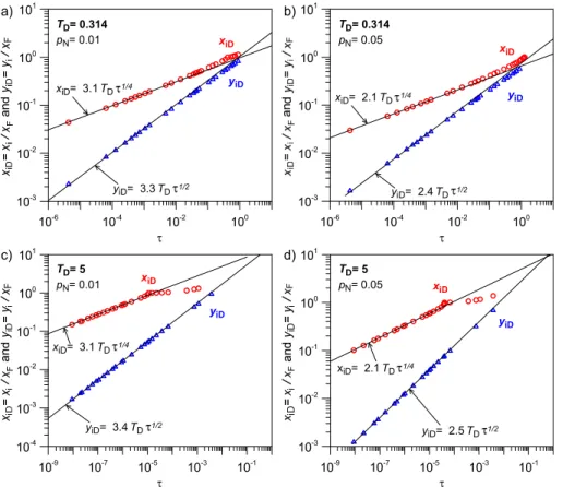
-axis and with the square root of time along the yD-axis for a certain time (Fig. 4).

During this time period the dimensionless distance of the normalized isobars on the

(13)

SED

5, 391–425, 2013

Title Page

Tables Figures

◭ ◮

Back Close

Full Screen / Esc

Discussion

P

a

per

|

Dis

cussion

P

a

per

|

Discussion

P

a

per

|

Discussio

n

P

a

per

|

xD-axis progresses according to

xiD(τ)=αbTDτ1/4 (12)

with the value of the constantαb depending on the chosen isobar, e.g. αb=3 and 2

for the normalized isobarspN=0.01 and 0.05, respectively. In dimensional variables,

Eq. (12) reads

5

x_i(t)=αb(Dbt)1/4 (13)

wherex_i(t) is the position of the isobar in the fracture for timetand

Db= T_F2 ηfkmsm

, (14)

here referred to as the bilinear flow diffusivity. This diffusivity combines fracture and matrix properties and has dimensions of L4/T. Equations (13) and (14) are specific

10

formulations of the self similarity of the pressure profiles in the fracture during bilinear flow found by Weir (1999).

The dimensionless distance of the normalized isobar on theyD-axis is given by

yiD=αmTDτ1/2 (15)

during bilinear flow corresponding to

15

yi =αm(Dmt)1/2 (16)

in dimensional variables. Combining Eqs. (12) and (15), the evolution of the ratio

yiD/xiD depends on dimensionless time as

yiD x_iD =

αm α_bτ

1/4

=α_αm

b Dm2 Db

!1/4

(14)

SED

5, 391–425, 2013

Title Page

Tables Figures

◭ ◮

Back Close

Full Screen / Esc

Discussion

P

a

per

|

Dis

cussion

P

a

per

|

Discussion

P

a

per

|

Discussio

n

P

a

per

The migration of the normalized isobars according to Eqs. (12) to (17) terminates for two di_fferent reasons depending on the size of the dimensionless fracture conductivity. The change in migration behavior occurs in the interval 1< TD<2 and we illustrate

the two types of terminations by considering two examples,TD=0.314 andTD=5, in

Fig. 4.

5

For dimensionless fracture conductivities lower than 1, the normalized isobars start to slightly accelerate relative to the fourth-root-of-time migration along thexD-axis long

before they reach the fracture tip, i.e.xD=1 (Fig. 4). Migration of the normalized

iso-bars in they-direction simultaneously slows down a little bit relative to the initial square-root-of-time migration (Fig. 4a, b). The curves ofxiD and yiD merge close to the

inter-10

ception of the two extrapolated diagnostic fourth-root and square-root relations actu-ally occurring at (τ≃1,xD=yD≃1). After merging the two curves follow the 1/2-slope

straight line indicating that radial flow conditions are approached.

For dimensionless fracture conductivities larger than 2 migration of the normalized isobars along thexD-axis decelerates and actually almost terminates for a finite time

15

interval when reaching the fracture tip and long before the interception of the two ex-trapolated diagnostic fourth-root and square-root relations (Fig. 4c, d). After some time, the migration finally accelerates again and appears to approach the straight line ofyiD

that closely follows a square-root-of-time relation. Upon closer inspection, one notices thatxiDslightly accelerates atxiD≃0.8, i.e. before the prominent halt in migration. This

20

intermittent acceleration is caused by the reflection of the isobar at the fracture tip that one can rationalize when invoking an image fracture at the fracture tip and an image well at a distance of 2xF producing or injecting at the same rate as the real well. The

“reflection” of the normalized isobar is then approximated by the superposition of the pressure fields of the two wells. Migration will accelerate when the isobars of the two

25

wells are approaching each other from both sides of the fracture tip.

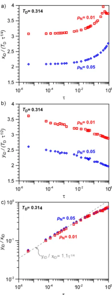
A more detailed view of the deviation of the normalized isobars from the fourth-root and square-fourth-root-of-time behavior is obtained by using normalized presentations,

xiD/TDτ 1/4

andyiD/TDτ 1/2

(15)

SED

5, 391–425, 2013

Title Page

Tables Figures

◭ ◮

Back Close

Full Screen / Esc

Discussion

P

a

per

|

Dis

cussion

P

a

per

|

Discussion

P

a

per

|

Discussio

n

P

a

per

|

presentations (Fig. 5a, b) confirm that normalizedxiD is constant for a certain time

in-terval and starts to bend upward in a similar way as the normalized well pressure bends downward (Fig. 2c). Normalized yiD is not constant even in the early stage

(τ≃10−6) but decreases continuously with a slight increase in slope at dimension-less timeτ≃10−2(Fig. 5b). The early deviation from the square root of time migration

5

indicates that even in the direction perpendicular to the fracture the pressure propaga-tion is affected by the presence of the fracture at all times. The width-to-length ratio of the normalized isobars (or pressure field),yiD/xiD, initially follows a fourth-root-of-time

relation (Fig. 5c) and subsequently bends clockwise from the 1/4-slope-straight line simultaneously with the upward bending of normalizedxiD. Within the resolution of our

10

numerical simulation this ratio is almost identical for all normalized isobars (Fig. 5c) suggesting that all normalized isobars have a similar shape and undergo the same evolution simultaneously in dimensionless time. The observed relationship between the ratioyiD/xiD and dimensionless time τ allows us to determine the width-to-length

ratio of all normalized isobars at any instant. During the bilinear flow period this ratio is

15

approximately given byyiD/xiD≃1.1τ 1/4

(Fig. 5c).

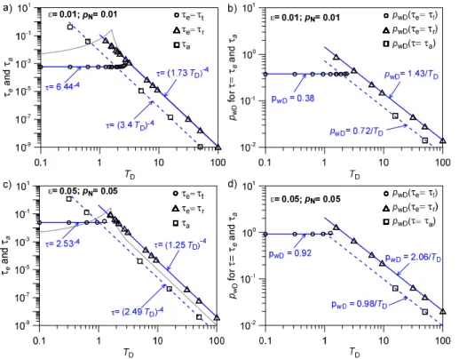
3.3 End time of bilinear flow from well pressure observations

For single-well tests, well pressure constitutes the only observable pressure and the end time of bilinear flow is generally determined by using its deviation from the 1/ 4-slope-straight line (in log-log plots of well pressure vs. time). According to our

observa-20

tions (Sect. 3.1), the type curve for the infinitely long fracture rather than the 1/ 4-slope-straight line represents the master curve, and only in its initial part up to dimensionless time τ≃10−6 this master curve is identical with the 1/4-slope-straight line. For later

times the master curve bends clockwise from the 1/4-slope-straight line due to the gradual transition from bilinear to radial flow. All type curves for fractures with finite

25

(16)

SED

5, 391–425, 2013

Title Page

Tables Figures

◭ ◮

Back Close

Full Screen / Esc

Discussion

P

a

per

|

Dis

cussion

P

a

per

|

Discussion

P

a

per

|

Discussio

n

P

a

per

curve, those forTD>10 in the straight-line section. We consequently introduce two

cri-teria for the termination of bilinear flow, one for the clockwise deviation of the master curve from the 1/4-slope-straight line and a second one for the counterclockwise de-viation from the master curve. According to the underlying mechanisms these criteria are addressed astransition criterion andreflection criterion, respectively. The time

de-5

termined by the transition criterion will be addressed astransition time, the time deter-mined by the reflection criterion asreflection time. In order to achieve higher accuracy in the determination of transition time and reflection time the two criteria are formulated for the normalized type-curvespwN=pwD/2.45τ

1/4

andp∞

wN=p∞wD/2.45τ 1/4

. Thetransition criterion

10

pwN=p∞_wN=1−ε (18)

addresses the clockwise deviation of type curves and master curve from the horizontal at unity, i.e. actual pressures fall short of the bilinear relation by a relative amount ofε

due to the transition to radial flow (Fig. 6). Unaffected by the fracture tip, the type curves under consideration are identical with the master curve before the transition criterion

15

is fulfilled. Accordingly the transition time is identical for all type curves complying with this criterion and in particular does not depend on dimensionless fracture conductivity

TD but only on the value of ε used (Fig. 7a, c). For each ε a maximum TD however

exists up to which the transition time can be determined. For type curves deviating from the master curve before the transition criterion is met the transition time cannot

20

be determined.

Thereflection criterion

pwN=(1+ε)p∞wN (19)

reflects the described reflection of normalized isobars at the fracture tip (Sect. 3.2) that produces the counterclockwise deviation of the normalized type curvespwN from the

25

normalized master curvep∞

wN (Fig. 6). Our data show that for normalized type curves

(17)

SED

5, 391–425, 2013

Title Page

Tables Figures

◭ ◮

Back Close

Full Screen / Esc

Discussion

P

a

per

|

Dis

cussion

P

a

per

|

Discussion

P

a

per

|

Discussio

n

P

a

per

|

with the curved deviation lines (Eq. 19) up to at leastε=0.05 and thus a reflection time τr can be determined. Type curves with TD<1 also show a reflection but the

associated deviation from the normalized master curve remains quite small and the reflection criterion may not be met for any ε of practical significance. The reflection time is proportional toT_D−4 for all type curves with TD>1 (Fig. 7). This relation is

in-5

tuitively understandable when recalling our observation that the normalized isobars in the fracture migrate proportional to τ1/4. The time it takes for a normalized isobar to propagate from the well to the fracture tip is therefore proportional tox_F4and sinceTDis

inversely proportional tox_F the observed relation between reflection time and dimen-sionless fracture conductivity results. For dimendimen-sionless fracture conductivitiesTD<1

10

this relation may no longer be valid since in these cases migration of the normalized isobars starts to accelerate relative to the fourth-root-of-time migration long before the reflection criterion is fulfilled.

The arrival time of a normalized isobarpNat the fracture tip is smaller than the

re-flection time by a factor of 16 (Fig. 7a, c) when the same value is used forε and pN

15

(e.g. ε=pN=0.05). This numerical relation can be explained by turning again to the

above introduced concept of an image fracture and an image well. In this concept, the reflection of the normalized isobar at the fracture tip is approximated by the superposi-tion of the normalized pressure profiles of the two wells. Inserting 2xFDinstead ofxFD

in Eq. (12) increases the time by the observed factor of 16.

20

During the bilinear flow period the dimensionless well pressure is proportional toτ1/4

and thus its values are constant for the transition time and proportional toT−1

D for the

reflection time (Fig. 7b, d). Dimensionless well pressures for the reflection time and for the time of arrival of the normalized isobar at the fracture tip di_ffer by a factor of 161/4=2.

25

The end time of bilinear flow reported by Cinco-Ley and Samaniego-V. (1981) dif-fers significantly from our time estimates for dimensionless fracture conductivities

TD<5 (Fig. 7). When reporting their three regimes, Cinco-Ley and Samaniego-V.

(18)

SED

5, 391–425, 2013

Title Page

Tables Figures

◭ ◮

Back Close

Full Screen / Esc

Discussion

P

a

per

|

Dis

cussion

P

a

per

|

Discussion

P

a

per

|

Discussio

n

P

a

per

reflects the shortcomings encountered when relying on a deviation from the 1/ 4-power relation without investigating the deviation in detail especially for type-curves with 1.6< T_D<2.5; end time apparently becomes a discontinuous function of T_D as reported in Cinco-Ley and Samaniego-V. (1981).

4 Discussion

5

Introducing the dimensionless timeτ according to Eq. (8) as an alternative to the ap-proach by Cinco-Ley and Samaniego-V. (1981), while leaving all other dimensionless parameters consistent with this previous analysis, proved to be favorable for a bet-ter understanding of bilinear flow. The new dimensionless time permits identification of a unique function of the dimensionless well pressure for an infinitely long fracture

10

(TD=0) applicable from the beginning of bilinear flow up to fully developed radial flow.

A normalized presentation of computed type curves for various dimensionless fracture conductivities showed that the type curve for the infinitely long fracture rather than the 1/4-slope-straight line, as assumed by Cinco-Ley and Samaniego (1981), constitutes the master curve for the type curves of all fractures with finite length. The latter all

15

deviate counterclockwise from the master curve instead of clockwise (for low fracture conductivity) or counterclockwise (for high fracture conductivity) from the 1/ 4-slope-straight line as assumed by these authors.

The master curve itself starts its clockwise deviation from the 1/4-slope-straight line at a dimensionless timeτ≃10−6. However, clockwise deviation builds up very slowly

20

and becomes noticeable in the commonly used log-log presentation only atτ_≃10−2. Furthermore, this clockwise deviation is counteracted by a counterclockwise bending for finite fractures. These counteracting effects are balanced best for fracture con-ductivities close to 2 so that these type-curves stay close to the 1/4-slope-straight line the longest explaining why the end times of bilinear flow given by Cinco-Ley and

25

(19)

SED

5, 391–425, 2013

Title Page

Tables Figures

◭ ◮

Back Close

Full Screen / Esc

Discussion

P

a

per

|

Dis

cussion

P

a

per

|

Discussion

P

a

per

|

Discussio

n

P

a

per

|

In order to distinguish the two types of processes that lead to a termination of bi-linear flow, transition to radial flow and isobar reflection at the fracture tip preceding the transition to intermittent formation linear flow, we replaced the term “end time” by the specifications “transition time” and “reflection time” and established corresponding criteria. Application of these criteria to normalized type curves is especially

advan-5

tageous for fractures with dimensionless conductivity between 1 and 2 since in this interval both, transition time and reflection time, can be determined. The transition time that is independent of dimensionless fracture conductivity can be determined for dimensionless fracture conductivities up to about 2; reflection time, inversely propor-tional to the fourth power of dimensionless fracture conductivity, can be determined for

10

dimensionless fracture conductivities down to about 1.

Investigating the migration of isobars for (effectively) infinite fractures we found that isobars normalized with respect to the well pressure migrate proportional toτ1/4along the x-axis (i.e. in the fracture) and approximately proportional toτ1/2along the y-axis (i.e. in the matrix perpendicular to the fracture) up to a dimensionless time τ≃10−2.

15

Their width-to-length ratio is close to 1.1τ1/4during this time period and is independent of dimensionless fracture conductivity. This relation approximately holds for all normal-ized isobars with pN<1 that therefore have similar shape at any instant. When τ is

known this simple relation allows for determination of the width-to-length ratio of the isobars at any instant. The ratio is 0.035 forτ≃10−6, when the first sign of deviation

20

from the fourth-root-of-time behavior of the well pressure is noticeable relying on the semi-log plots of normalized well pressure (Figs. 2c and 6). For τ≃10−2 when the deviation becomes noticeable in conventional log-log presentations the ratio amounts to 0.35. Thus, in a strict sense bilinear flow ends at a very early state of the shape evolution but the termination becomes noticeable in conventional type curves only at a

25

(20)

SED

5, 391–425, 2013

Title Page

Tables Figures

◭ ◮

Back Close

Full Screen / Esc

Discussion

P

a

per

|

Dis

cussion

P

a

per

|

Discussion

P

a

per

|

Discussio

n

P

a

per

approach 1 for true radial flow in case of the infinite fracture, a suggestion that has to be checked by further studies.

For finite fractures the shape evolution is disturbed when the isobars approach the fracture tip by a process here described as “reflection”. This reflection is noticed by a clockwise deviation of the well pressure from the master curve at a time sixteen

5

times later than its actual occurrence at the fracture tip. Interestingly, the disturbance in the shape evolution shortens the time it takes to approach radial flow conditions characterized by a width-to-length ratio of 1. This shortening can be explained by the fact that migration of the isobars along the x-axis is retarded after passing the fracture tip.

10

5 Implications for well test analysis

Our findings may be used to determine geometric and hydraulic properties of fracture and matrix from short injection and production tests for which conventional well-test analysis would not be applicable. However, this evaluation requires excellent test con-ditions and high-quality pressure data. We recommend analyzing plots of normalized

15

well pressure (Fig. 6) in addition to the conventional log-log plots and derivative (exem-plified in Fig. 2 a, b). Using these normalized plots one may obtain the desired infor-mation on fracture transmissibility, matrix permeability, and fracture length at a much earlier time than with conventional procedures as explicitly outlined below.

The first step of any analysis is to determine the slopeM characterizing the bilinear

20

flow section of a diagram of the change in well pressure vs. fourth root of time (∆pw= Mt1/4). The slope is then used to construct a ∆pw/Mt

1/4

vs. time diagram. In case bilinear flow ended during the pumping operation (indicated by either a clockwise or an counterclockwise deviation from a horizontal line at 1), transition time (tt) and/or

reflection time (tr) and the corresponding well pressure (pwt and/or pwr) can be read

25

(21)

SED

5, 391–425, 2013

Title Page

Tables Figures

◭ ◮

Back Close

Full Screen / Esc

Discussion

P

a

per

|

Dis

cussion

P

a

per

|

Discussion

P

a

per

|

Discussio

n

P

a

per

|

or Eq. (19). The following cases and their potential for determining fracture and matrix characteristics have to be distinguished:

Case 1: When the well pressure record constrains only the slopeM, then the product

TF(kmsm) 1/2

can be determined using

TF(kmsm)1/2= 

 qwη

3/4 f Mh



 2

. (20)

5

Case 2: When the well pressure record exhibits a clockwise deviation of relative magnitude ε, i.e. the transition time is known, then the permeability of the matrix km

can be determined from

km= qwηf

2πh pwtD

pwt

(21)

wherepwtD=0.38, 0.68 and 0.92 for ε=0.01, 0.03, and 0.05, respectively (Fig. 7b,

10

d). In case the storage coefficient of the matrix, sm, is known or can be reasonably

estimated, the fracture conductivity can be derived by

T_F= 1

(kmsm)1/2 

 qwη

3/4 f Mh



 2

. (22)

Then, also the two diffusivities of the system, the one for bilinear flowDb(Eq. 14) and

the one for the matrixDm, are constrained. Furthermore, the ratioyiD/xiD(oryi/xi) can

15

be determined from

yiD xiD =

αm αF

τe1/4≃1.1τ 1/4

t . (23)

The dimensionless fracture conductivity obeys the relation TD< TD maxwith TD max=

2.5, 1.6, and 1.0 for ε=0.01, 0.03, and 0.05, respectively, and thus one also has a constraint on fracture length, i.e.xF> TF/TD maxkm.

(22)

SED

5, 391–425, 2013

Title Page

Tables Figures

◭ ◮

Back Close

Full Screen / Esc

Discussion

P

a

per

|

Dis

cussion

P

a

per

|

Discussion

P

a

per

|

Discussio

n

P

a

per

Case 3: When the pressure record contains a counterclockwise deviation of rela-tive magnitude εbut no clockwise deviation, then one knows the reflection time and has the relationTD>10. The dimensionless fracture conductivityTDcannot be further

constrained, however, since all type curves rapidly rise in a similar way. Thus, only the productTF(kmsm)

1/2

can be determined (as in case 1). In addition, if the matrix

5

properties (k_mands_m) are known or can be reasonably estimated one can infer

xF=C

T_F2 kmηfsm

tr !1/4

=C(Dbtr)1/4 (24)

from the reflection time where C=1.73, 1.41, and 1.25 for ε=0.01, 0.03, and 0.05, respectively (Fig. 7a, c).

Case 4: when the pressure record exhibits a clockwise deviation from the 1/

4-slope-10

straight line succeeded by a counterclockwise deviation from the master curvep∞_wN, then transition time as well as reflection time are known. Such data allows for deter-mination of matrix permeability, fracture transmissibility, and the ratioy_i/x_i (as in case 2). In addition, the dimensionless fracture conductivityTDcan be quantified by looking

for a pair of matching transition times and reflection times in Fig. 7 and with that the

15

fracture lengthxFcan be determined according to

x_F= TF

kmTD

. (25)

6 Conclusions

Using two-dimensional numerical modeling we investigated the evolution of the pres-sure field in and around a fracture imbedded in a permeable matrix during injection

20

(23)

SED

5, 391–425, 2013

Title Page

Tables Figures

◭ ◮

Back Close

Full Screen / Esc

Discussion

P

a

per

|

Dis

cussion

P

a

per

|

Discussion

P

a

per

|

Discussio

n

P

a

per

|

dimensionless time containing only the transport parameters of fracture and matrix as well as the storage coe_fficient of the matrix but no geometrical or storage parame-ters of the fracture. In this presentation, type curves of dimensionless well pressure for fractures with finite length evolve from a single master curve when dimensionless time progresses. The unique master curve corresponds to an infinitely long fracture and

5

comprises two stages with an extended transition in-between. The early and the late stage are characterized by pressure in the well increasing with time to a power of 1/4 (bilinear flow) and the logarithm of time (radial flow), respectively. For fractures of finite length, well pressure always deviates from the master curve towards higher pressures, i.e. all type curves branch offcounterclockwise from the master curve instead of

clock-10

wise or counterclockwise from the 1/4-slope-straight line as considered by Cinco-Ley and Samaniego-V. (1981). Nevertheless, two mechanisms have to be distinguished for the termination of bilinear flow depending on fracture and matrix properties.

For any fracture of finite length, the propagation of the pressure front in the fracture will eventually be affected by the fracture tip. Fractures with a dimensionless

conduc-15

tivityTD>10 qualify as fractures with high conductivity since for these the reflection

of the pressure front at the fracture tip happens long before substantial migration of isobars in the matrix. The reflection leads to a reduction of the pressure gradient in the fracture and thus signals the transition to formation linear flow. Termination of bilinear flow is noticed by an increase of well pressure relative to the horizontal section of the

20

normalized master curve that occurs however only 16 times later than the actual reflec-tion at the fracture tip. In contrast, for fractures with low conductivity (TD<1) migration

of isobars in the matrix becomes significant long before the pressure front in the frac-ture approaches the fracfrac-ture tip due to the difference in the power in the relation with time, i.e. square root and fourth root for matrix and fracture, respectively. The gaining of

25

(24)

SED

5, 391–425, 2013

Title Page

Tables Figures

◭ ◮

Back Close

Full Screen / Esc

Discussion

P

a

per

|

Dis

cussion

P

a

per

|

Discussion

P

a

per

|

Discussio

n

P

a

per

the fracture. For an intermediate range of fracture conductivities (1< TD<10),

reflec-tion at the fracture tip interferes with the transireflec-tion to radial flow and normalized well pressure exhibits a peculiar succession of decrease, increase, and decrease in cases. The two criteria introduced for the deviation of the master-curve from the fourth-root-of-time behavior (transition criterion) and for the deviation of the type curves for finite

5

fractures from the master curve (reflection criterion) revealed that the transition time is independent of the dimensionless fracture conductivity and applies to the infinite frac-ture as well as to all finite fracfrac-tures whose type curves do not branch o_fffrom the master curve before this end time is reached. The reflection time is inversely proportional to dimensionless fracture conductivity to a power of 4 corresponding to the

fourth-root-of-10

time migration of the normalized isobars in the fracture expressed by a scaling relation that includes a bilinear diffusivity with dimensions ofL4/t.

The gained insight into the relation between the entire flow field and the peculiari-ties of the recorded wellbore pressure permits constraining hydraulic and geometrical parameters of the subsurface in practice. Using semi-log plots of normalized well

pres-15

sure in addition to the common log-log diagrams improves the sensitivity of analyses in particular for dimensionless fracture conductivities smaller than 3 and hydraulic pa-rameters of matrix and fracture may be determined after shorter test duration than necessary for conventional analysis.

Acknowledgements. Generous funding by the German science foundation (DFG) within the

20

collaborative research centre “Rheology of the earth” (SFB 526) is gratefully acknowledged.

References

Boonstra, J. and Boehmer, W. K.: Analysis of data from aquifer and well tests in intrusive dikes, J. Hydrol., 88, 301–317, 1986.

Bourdet, D.: Well Test Analysis: The Use of Advanced Interpretation Models, Elsevier,

Amster-25

(25)

SED

5, 391–425, 2013

Title Page

Tables Figures

◭ ◮

Back Close

Full Screen / Esc

Discussion

P

a

per

|

Dis

cussion

P

a

per

|

Discussion

P

a

per

|

Discussio

n

P

a

per

|

Butler Jr., J. J. and Liu, W. Z.: Pumping tests in non-uniform aquifers – the linear strip case, J. Hydrol., 128, 69–99, 1991.

Chaudhry, A. U.: Oil Well Testing Handbook, Elsevier, Amsterdam, 2004.

Chen, L. and Talwani, P.: Reservoir-induced seismicity in China, Pure Appl. Geophys., 153, 133–149, 1998.

5

Cinco-Ley, H. and Samaniego-V., F.: Transient pressure analysis for fractured wells, J. Pet. Technol., 33, 1749–1766, 1981.

Cinco-Ley, H., Samaniego-V., F., and Dominguez-A., N.: Transient pressure behavior for a well with a finite-conductivity vertical fracture, Soc. Petrol. Eng. J., 18, 253–264, 1978.

Dake, L.: The Practice of Reservoir Engineering, vol. 36, Elsevier, Amsterdam, 2001.

10

Deichmann, N. and Ernst, J.: Earthquake focal mechanisms of the induced seismicity in 2006 and 2007 below Basel (Switzerland), Swiss J. Geosci., 102, 457–466, 2009.

Du, K. and Stewart, G.: Bilinear flow regime occurring in horizontal wells and other geological models, in: International Meeting on Petroleum Engineering, Beijing, China, 111–118, 1995. Earlougher Jr, R. C.: Advances in Well Test Analysis, vol. 5, Society of Petroleum Engineers,

15

Richardson, TX, 1977.

Gringarten, A. C.: Interpretation of transient well test data, in: Developments in Petroleum En-gineering, 133–196, edited by: Dawe, R. A. and Wilson, D. C., Elsevier, London, 1985. Hainzl, S., Kraft, T., Wassermann, J., Igel, H., and Schmedes, E.: Evidence for rainfall-triggered

earthquake activity, Geophys. Res. Lett., 33, L19303, doi:10.1029/2006GL027642, 2006.

20

H ¨aring, M. O., Schanz, U., Ladner, F., and Dyer, B. C.: Characterisation of the Basel 1 enhanced geothermal system, Geothermics, 37, 469–495, 2008.

Horne, R. N.: Modern Well Test Analysis, a Computer-Aided Approach, Petroway Inc., Palo Alto, CA, 1995.

Jelmert, T. A. and Vik, S. A.: Bilinear flow may occur in horizontal wells, Oil Gas J., 93, 57–59,

25

1995.

Jenkins, D. N. and Prentice, J. K.: Theory for aquifer test analysis in fractured rocks under linear (nonradial) flow conditions, Ground Water, 20, 12–21, 1982.

Jung, R. and Weidler, R.: A conceptual model for the stimulation process of the HDR-System at Soultz, Geoth. Res. T., 24, 143–147, 2000.

30

(26)

SED

5, 391–425, 2013

Title Page

Tables Figures

◭ ◮

Back Close

Full Screen / Esc

Discussion

P

a

per

|

Dis

cussion

P

a

per

|

Discussion

P

a

per

|

Discussio

n

P

a

per

Matthews, C. and Russell, D. G.: Pressure Buildup and Flow Tests in Wells, vol. 1, Society of Petroleum Engineers, 1967.

Ortiz, A., Jung, R., and Renner, J.: Hydromechanical analyses of the hydraulic stimulation of bore-hole Basel 1, Geophys. J. Int., 185, 1266–1287, 2011.

Riley, M. F.: Finite conductivity fractures in elliptical coordinates, Ph. D. thesis, Stanford

Univer-5

stity, Stanford, 1991.

Rushing, J. A., Sullivan, R. B., and Blasingame, T. A.: Post-fracture performance diagnostics for gas wells with finite conductivity vertical fractures, SPE 97972, 2005.

Saar, M. O. and Manga, M.: Seismicity induced by seasonal groundwater recharge at Mt. Hood, Oregon, Earth Planet. Sci. Lett., 214, 605–618, 2003.

10

Shapiro, S. A. and Dinske, C.: Fluid-induced seismicity: pressure diffusion and hydraulic frac-turing, Geophys. Prospect., 57, 301–310, 2009.

Stright, D. and Gordon, J.: Decline curve analysis in fractured low permeability gas wells in the Piceance basin, in: SPE/DOE Low Permeability Gas Reservoirs Symposium, 351–362, Denver, Colorado, 1983.

15

Theis, C. V.: The relation between the lowering of the piezometric surface and the rate and duration of discharge of a well using groundwater storage, Trans. AGU, 16, 519–524, 1935. Verga, F. M. and Beretta, E.: Transient dual porosity behavior for horizontal wells: case histories,

in: SPE Annual Technical Conference and Exhibition, New Orleans, Louisiana, 2001. Weir: Single-phase flow regimes in a discrete fracture model, Water Resour. Res., 35, 65–73,

20

1999.

Zimmermann, G., Huenges, E., Saadat, A., Legarth, B., Bl öcher, G., Reinicke, A., Milsch, H., Holl, H.-G., Moeck, I., K öhler, S., and Brandt, W.: Enhancement of productivity after reservoir stimulation of the hydro-thermal reservoir Gross Sch önebeck with different fracturing con-cepts, in: Engine Workshop 3: Stimulation of Reservoir and Induced Microseismicity, 81–86,

25

(27)

SED

5, 391–425, 2013

Title Page

Tables Figures

◭ ◮

Back Close

Full Screen / Esc

Discussion

P

a

per

|

Dis

cussion

P

a

per

|

Discussion

P

a

per

|

Discussio

n

P

a

per

|

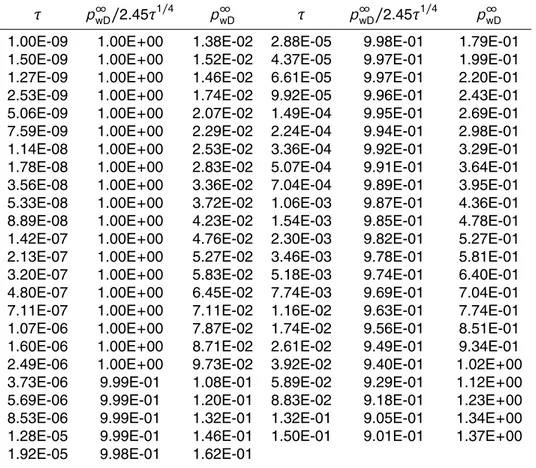
Table 1.Values of the master curve for normalized well pressurep∞

wD/2.45τ 1/4

(Figs. 2c, 6)

τ p∞

wD/2.45τ 1/4

p∞

wD τ p∞wD/2.45τ

1/4

p∞

wD

(28)

SED

5, 391–425, 2013

Title Page

Tables Figures

◭ ◮

Back Close

Full Screen / Esc

Discussion

P

a

per

|

Dis

cussion

P

a

per

|

Discussion

P

a

per

|

Discussio

n

P

a

per

Table 2.Nomenclature.

bF fracture width [m] C constant [–]

Db effective hydraulic diffusivity of fracture during bilinear flow, Eq. (14), [m 4

s−1]

DF hydraulic diffusivity of (isolated) fracture,DF=TF/ηfSF[m 2

s−1]

Dm hydraulic diffusivity of matrix, Dm=km/ηfsm [m

2 s−1]

h height of the open well section, fracture height, [m]

km matrix permeability [m 2

]

paD dimensionless pressure atτa peD dimensionless pressure atτe

pN normalized pressure difference, Eq. (11), [–] prD dimensionless pressure atτr

pw well pressure, [Pa]

∆pw change in well pressure difference, [Pa] pwD dimensionless well pressure, Eq. (7), [–] p∞

wD master curve for dimensionless well pressure (Figs. 2c and 6) [–] pweD dimensionless well pressure at end time of bilinear flow, [–]

pwN normalized well pressure, i.e. normalized by the 1/4-relation for bilinear flow, [–] qw flow rate in the well [m

3 s−1]

sm specific storage capacity of matrix [Pa −1

]

SF storativity of the fracture [mPa −1

]

t time, [s]

TF fracture conductivity (transmissibility), [m 3

]

TD dimensionless fracture conductivity, Eq. (9), [–]

x,y spatial coordinates along, normal to the fracture with origin at the well, [m]

xF fracture half length, [m]

xD,yD dimensionless coordinates (xD=x/xF,yD=y/xF) [–]

xiD,yiD dimensionless distances of normalized isobars from the well (along thexD- andyD-axis respectively) [–] Greek symbols

αb constant for pressure diffusion in fracture during bilinear flow, Eq. (12), [–] αm constant for pressure diffusion in matrix, Eq. (15), [–]

Γ gamma function [–]

ηf fluid viscosity, [Pa s]

τ dimensionless time, Eq. (8), [–]

τa dimensionless arrival time (of the normalized isobar at the fracture tip) [–] τe dimensionless end time of bilinear flow [–]