Abstract
An in-depth study has been carried out for the dispersion of Love waves in an isotropic elastic layer sandwiched between orthotropic and prestressed inhomogeneous elastic half-spaces. The inhomogene-ities in density and rigidity of the lower half-space are space depend-ent and an arbitrary function of depth. Simple mathematical tech-niques are used to obtain dispersion relation for Love wave propaga-tion in an isotropic layer. An extensive analysis is carried out through numerical computation to explore the effect of inhomogeneity and initial stress the lower half on the phase velocity of the Love waves. The numerical analysis of dispersion equation manifests that the phase velocity of the Love wave increases with the increase of stress parameter. The results further indicate that the inhomogeneity of the half space affect the wave velocity significantly. These results can be useful to study geophysical prospecting and understanding the cause and estimation of damage due to earthquakes.
Keywords
Love wave; initial stress; inhomogeneity; variable density.
Dispersion of Love wave in an isotropic layer sandwiched between
orthotropic and prestressed inhomogeneous half-spaces
1 INTRODUCTION
The deformation at any point of the medium is useful to analyze the deformation field around mining tremors and drilling into the crust of the earth. It may also find application in various engineering problems, crystal physics and solid-earth geophysics regarding deformation of an anisotropic solid. In fact, study of surface waves in non-homogeneous and layered media has been of central interest to theoretical and experimental seismologists. Our Earth is a spherical and layered solid under high initial stress. Due to variation of temperature, gravitating pull, atmosphere, slow process of creep and pressure due to crustal layer, the critical initial stresses are stored in the layer of the Earth. At the present time the usefulness of dislocation theory in seismology is restricted by the absence of detailed knowledge of either the tectonic stress which drives the system or the stress which resists slip on the fault plane and by the absence of detailed observations of deformation preceding, accompanying of dislocation theory to seismology lie in the mathematical theory but
Rajneesh Kakar
Department of Physics, GNA University, Phagwara-144405, India
Corresponding author: [email protected]
http://dx.doi.org/10.1590/1679-78251918
rather in the basis mechanics of faulting. The stresses which exist in an elastic body even though the external forces are absent are termed as prestresses. These stresses might exert significant effect on the elastic waves produced by earthquakes. The propagation of Love waves in a non-homogeneous elastic media is of considerable importance in earth-quake engineering and seismology on account of occurrence of non-homogeneities in the earth crust, as the earth is made up of different layers. The mathematical expression provides the bridge between modelling results and field applications.
Surface waves are very important in the study of earthquake engineering, geophysics and geodynamics. Love waves cause more destruction to the structure than that of the body waves due to its slower attenuation of the energy. The supplement of surface wave analysis and other wave propagation problems to anisotropic elastic materials has been the subject of many studies. Many authors have discussed Love wave propagation by considering various irregularities, inhomogeneities and boundaries of the Earth. Love (1944) and Ewing et al. (1957) proposed the propagation of waves in transversely isotropic medium. Chatopadhyay (1975) discussed Love waves due to irregularity in the thickness of the non- homogeneous crystal layer. Deresiewicz (1962) studied the propagation of Love waves in a homogeneous crust overlying an inhomogeneous substratum. Bhattacharya (1969) examined the Love waves in intermediate heterogeneous layer placed between isotropic elastic half-spaces. Midya (2004) discussed Love waves in micropolar homogeneous elastic media. Manna et al. (2013) discussed propagation of Love wave in hetrogeneous elastic half-space and piezoelectric layer. Du et al. (2008) studied the effect of initial stress on the propagation of piezoelectric layered structures loaded with viscous liquid. Liu and Wang (2005) studied Love waves in functionally graded layered piezoelectric structure. Chakraborty and Dey (1982) discussed the propagation of Love waves in water saturated soil underlain by heterogeneous elastic medium. Ke et al. (2005) discussed Love waves in nonhomogeneous fluid saturated porous layered half-space. Kundu et al. (2013) discussed propagation of Love wave in porous rigid layer kept over prestressed half space. Chattaraj et al. (2013) discussed Love wave propagation in irregular prestressed anisotropic porous stratum. Ghorai et al. (2010) showed the effect of rigid boundary on the propagation of Love wave in porous layer placed over an elastic half-space. Kadian and Singh (2010) studied the influence of size of barrier on Love wave reflection. Ahmed and Abd-Dahab (2010) studied the effect of initial stress on Love waves in an orthotropic Granular layer. Gupta et al. (2013) proposed a mathematical model to study Love wave propagation in homogeneous and initially stressed hetrogeneous half-spaces. Presently, Madan et al. (2014) investigated propagation of Love waves in saturated porous anisotropic layer. Kakar and Gupta (2014) studied Love waves in an intermediate heterogeneous layer lying in between homogeneous and inhomogeneous isotropic elastic half-spaces. More recently, Kundu et al. (2014a; 2014b) have examined Love wave propagation in fiber-reinforced media.
The present paper deals with the study of propagation of Love wave in a sandwiched layer lying between orthotropic and inhomogeneous half spaces. Five different cases have been studied for propagation of Love waves in a layer. The dispersion equations of Love waves under assumed conditions have been derived. Also numerical computation of dispersion equation has been performed to show the effect of initial stresses and inhomogeneity parameters on the propagation of Love waves. It has been found that initial stress parameter, rigidity parameter and density parameter of the lower half-space affect the phase velocity of Love waves.
2 FORMULATION OF THE PROBLEM
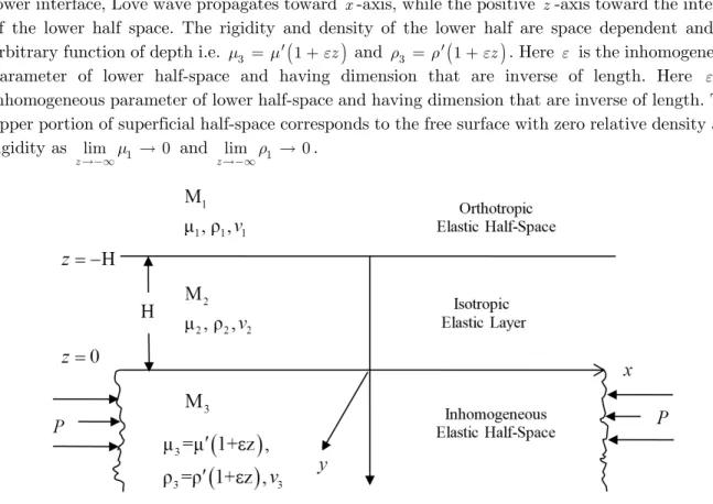
We have considered an isotropic and homogeneous layer of thickness H (denoted as M2) sandwiched between two orthotropic and prestressed inhomogeneous (denoted as M1 and M3)
half-spaces (as shown in Fig. 1). Let 2 and 2 be the rigidity and density of the intermediate layer and rigidity and density in the upper half-space are 1 and 1. The origin has been taken at the lower interface, Love wave propagates toward x-axis, while the positive z-axis toward the interior of the lower half space. The rigidity and density of the lower half are space dependent and an arbitrary function of depth i.e. 3
1z
and 3
1z
. Here is the inhomogeneous parameter of lower half-space and having dimension that are inverse of length. Here is inhomogeneous parameter of lower half-space and having dimension that are inverse of length. The upper portion of superficial half-space corresponds to the free surface with zero relative density and rigidity as lim 1 0z and zlim 1 0.
Figure 1: Geometry of the problem.
3 SOLUTION OF THE PROBLEM 3.1 Solution for the upper half-space
Equation of motion for upper half-space in the absence of body forces can be written as (Love, 1911)
2 1
1 2
2 1
1 2
2 1
1 2
xy
xx xz
yx yy yz
zy
zx zz
u
x y z t
v
x y z t
w
x y z t
(1)
where xx, , , , , , , xy xz yx yy yz zx zy and zz are the incremental stress components, u1, v1 and 1
w are the components of the displacement vector in the upper layer, 1 is the density of the upper half-space.
The stress–strain relations are
2
2
2
xx xx xx xy yy xz zz
xy z xy
yy yx xx yy yy yz zz
yz x yz
zz zx xx zy yy zz zz
zx y zx
e e e
e
e e e
e
e e e
e
(2)
where xx, , , , , , , xy xz yx yy yz zx zy and zz are the incremental normal elastic coefficients,
,
x
y and z shear modulus along x, y and z axis respectively. The strain components exy,
,
xx
e eyy, eyz, ezx and ezz are defined by
1 1 1 1 1 1
1 1 1
1 1 1
, , ,
2 2 2
, ,
xy yz zx
xx yy zz
v u w v v w
e e e
x y y z z x
u v w
e e e
x y z
(3)
Using Love wave conditions u1 w1 0, v1 v x z t1( , , ) in equations (1) and (2), the equation of
motion for the upper orthotropic half-space becomes
2
2 2
1
1 1
1
2 2 2
z x
v
v v
x z t
(4)
and stress–strain relations reduces to
0
2 , 2
xx xy xz yy zx zy zz
yx z xye yz x yze
(5)
To solve Eq. (4) we take the following substitution
1 U(z)exp ( )
v itkx (6)
where kc,c is phase velocity , c1 1 1 and k is wave number. Using Eq. (6) in Eq. (4), we get
2
2 2
d U( )
U( ) 0 d
z
z
z (7)
where 2 2
2
1 z x
k
c
(8)
Therefore, the solution for the upper orthotropic half-space is given by
1 A e exp ( ) z
v itkx (9)
where is arbitrary constant.
3.2 Solution for the lower half-space
Equation of motion for lower half-space under initial stress P acting along x-axis can be written as (Love, 1911)
2 3
3 2
2 3
3 2
2 3
3 2
z y
xy
xx xz
z
yx yy yz
y zy
zx zz
u P
x y z y z t
v P
x y z x t
w P
x y z x t
(10)
where xx, , , , , , , xy xz yx yy yz zx zy and zz are the incremental stress components, u3, v3 and
3
w are the components of the displacement vector and 3is the density of the lower half-space. Here, x, y and zare the rotational components in the lower half-space, which are defined by
3 3
3 3
3 3
1 2
1 2
1 2 x
y
z
w v
y z
u w
z x
v u
x y
(11)
Using Love wave conditions u3 w3 0, v3 v x z t3( , , ), Eq. (10) can be reduced to
2 2
3 3
3
2 2
2
yx yz P v v
x z x t
(12)
The stress–strain relations are
3 3
3 3
3 3
3 3
0
1
2 2
2
1
2 2
2
xx yy xz zz
yx xy
yz yz
v u
e
x y
w v
e
y z
(13)
The inhomogeneity of rigidity and density of the lower half-space are
3 1 z
, 3
1z
(14)Now, substituting the inhomogeneity of rigidity from Eq. (14) in Eq. (13), we have
3
3
1 1
yx
yz
v z
x v z
z
(15)
The equation of motion (12) with the help of equations (14) and (15) can be written as
2 2 2
3 3 3 3
2 2 2
1
2 (1 ) 1
v v v v
P
z x x z z t
(16)
To solve Eq. (16) we take the following substitution
3 V(z)exp ( )
v itkx (17)
Using Eq. (17) in Eq. (16), we get
2
2 2
2
d V( ) dV( )
1 V( ) 0
1 d 2 (1 )
d
z z P
c k z
z z z
z
(18)
Introducing V( )z ( )z
1z
into Eq. (18) to cancel the term dV( ) dz z, we have
2 2 2
2
2 2 2
3 d ( )
1 ( ) 0
2 (1 )
d 4 1
z P c
k z
z
z z c
(19)
where c is phase velocity and c3 .
Introducing the non-dimensional quantities
1 2 2
2 3
1
2 (1 )
P c
r
z c
, s 2 (1rk z)
and kc
in Eq. (19), we get,
2
2 2
d 1 1
( ) 0 4
d 4
s
s r
s s
(20)
Eq. (20) is the well known Whittaker’s equation (Whittaker and Watson,1990). The solution Eq. (20) is given by
,0 1 ,0
( )s BWr ( )s Wr ( s)
(21)
where and 1 are arbitrary constants and Wr,0( )s , Wr,0(s) are the Whittaker functions. Now
considering the condition V( )z 0 as z i.e. ( )s 0 as s in Eq. (21), the exact solution becomes
,0 ( )s BWr ( )s
(22)
The solution of Eq. (22) is given by
,0 3
B ( )
V(z) exp ( ) exp ( )
(1 )
r W s
v i t kx i t kx
z
(23)
Eq. (23) is the displacement for the Love wave in the half space. Now, expanding Eq. (23) up to linear term, we have
- (1 )
3
1
e exp ( )
(1 ) 8 (1 )
rk z
v i t kx
z rk z
(24)
3.3 Solution for the intermediate isotropic layer
Equation of motion for intermediate layer can be written as (Love, 1911)
2 2
2 2
2 2
2 2
2 2
2 2
xy
xx xz
yx yy yz
zy
zx zz
u s
s s
x y z t
v
s s s
x y z t
w s
s s
x y z t
(25)
wheresxx, sxy, sxz, syx, syy, syz, szx, szy and szz are the incremental stress components, u2, v2 and w2 are the components of the displacement vector and 2 is the density of the intermediate layer.
The stress displacement relation for isotropic media is
2
e 2
ij ij ij
s e (26)
where and 2 are known as Lame’s constants for homogeneous media, ij is Kronecker delta and e u2 x v2 y w2 z is cubical dilatation. Here, eij
ui xj uj xi
2where, ui are the components of displacement vector and can be defined as
2 2
1 1
, , 0
2 2
xy yz zx xx yy zz
v v
e e e e e e
x z
(27)
Using Love wave conditions u2 w2 0, v2 v x z t2( , , ), the stress–strain relations are
2 2
2 2
0
xx yy xz zz
xy
yz
s s s s
v s
x
v s
z
(28)
Using Eq. (28), the Eq. (25) can be written as
2
2 2
2
2 2
2 2 2 2
2 1 v
v v
x z c t
(29)
where c2 2 2 .
To solve Eq. (29) we take the following substitution
2 W(z)exp ( )
v i tkx (30)
where kc, c is phase velocity and k is wave number. Using Eq. (30) in Eq. (29), we get
2
2 2
d W( )
W( ) 0 d
z
z
z (31)
where 2 2 2 2 2
1
c k
c
(32)
Therefore, the solution for the intermediate layer is given by
2 C cos D sin exp ( )
v z z itkx (33)
where C and D are arbitrary constants.
4 BOUNDARY CONDITIONS
Both displacement and stress components are continuous at z 0 and z , therefore the geometry of the problem leads to the following conditions:
1st Boundary conditions
(i) At the interface, z 0 the continuity of the displacement along the x direction requires that
2 3
v v , where v2 and v3 are the displacement components, along the y direction only, in the intermediate layer and lower half-space respectively.
(ii) At the interface, z 0 the continuity of the stress requires that
2 3
yz yz
s
, where syz
the relevant is stress component.
(iii)Also, stability conditions leads to v3 0 as z . 2nd Boundary conditions
(i) At the interface, z , the upper boundary plane is not free surface, the continuity of the displacement along thex direction requires that v1 v2, where v1 is the displacement component in the upper half-space along the y direction only.
(ii) At the interface, z , the continuity of the stress requires that
1 2
yz syz
, where
yz
the relevant is stress component.
(iii) Also, stability conditions leads to v1 0 as z . 5 DISPERSION RELATIONS
Applying 2nd boundary conditions in equations (2), (28) and equations (9), (33), we have
2
e
A x C sin D cos 0
(34)
A e C cos D sin 0 (35)
Now, applying 1st boundary conditions in equations (15), (28) and equations (24), (33), we have
1
2
2
D 1 1 1 0
kr
kr kr kr
e kr
(36)
2
C 1 0
kr kr kr e
(37)
Eliminating A, B, C and Dfrom equations (34) to (37), the dispersion relation for Love waves can
be calculated as
1 2 2 2 1 2 2e 1 1 1 sin
2
e 1 1 1
kr x
kr
kr kr kr
e kr
kr kr kr
e kr
1
2
cos
2
1 1 e cos e sin 0
kr
x
kr kr
e kr
On solving further above equation, we get
1 2 2 2 1 2 2e 1 1 1 tan
2
e 1 1 1
kr x
kr
kr kr kr
e kr
kr kr kr
e kr
2 2 2e 1 e 1 tan 0
kr kr
x e kr kr kr e kr kr kr
which implies
1
2 2 2
1
2
2
e 1 1 1 1 tan
1 2
e 1 1 1
kr
x
kr
kr kr kr
e kr
kr kr kr
e
x 0
(38)
On solving further equation (38), we get
1 2 1 2 2 2 1 1 tan 1 1 x x kr kr kr kr which implies1 2 2 2 2 2 2 2 1
2 2 2 2
2 1
1 1 1
tan 1 1 1 1 x z x x z x c kr
k k c kr
c c
k
c kr
k r c k
2 2 2 2 1 c c 1 2 2 2 2 2 1 2 2 2 2 2 2
1 1 1 1
1 1 1 1
z x x z z x x z
c c kr
r c
c kr c
r c 1 2 2 2 2
2 2 1 2 2
2 2 2
2 2
2
1 1 1
tan 1 1
1 1 1 1
z x x z z x x z c kr r c c k
c c kr c c
r c
(39)
Eq. (39) is dispersion relation of Love waves in an intermediate isotropic vertical layer placed in between orthotropic and prestressed inhomogeneous half-spaces.
Special cases
Case 1 If x z 1, the Eq. (39) reduces to
1 2 1 2 2 2 1 2
2 2 2 1 2
2 2 2
2 2 1 2
2 1
1 1 1
tan 1
1 1 1 1
c kr
r c
c c
k
c c c kr c
r c c 1
(40)
Eq. (40) is dispersion relation of Love waves in an intermediate isotropic vertical layer placed in between homogeneous and prestressed inhomogeneous half-spaces.
Case 2 If 0, the Eq. (39) reduces to
1
2 2 2
2
2 2
3
2
2 1 2
2 2 2 2 2 2
2
2 2 2
2 3
1 1
2
tan 1 1
1 1 1
2 z x x z z x x z
c P c
c
c c
k
c c
c P c c
c c (41)
Eq. (41) is dispersion relation of Love waves in an intermediate isotropic vertical layer placed in between orthotropic and prestressed homogeneous half-spaces.
Case 3 If x z 1, 0 the Eq. (39) reduces to
1
2 2 2
1 2 2
2 2
1 3
2
2 1 2
2 2 2 2 2 2
2
2 2 1 2 2
2 3 1
1 1
2
tan 1 1
1 1 1
2
c P c
c c
c c
k
c c
c P c c
c c c
(42)
Eq. (42) is dispersion relation of Love waves in an intermediate isotropic vertical layer placed in between homogeneous and prestressed homogeneous half-spaces.
Case 4 If 0, P 0, the Eq. (39) reduces to
1
2 2 2
2
2 2
3
2
2 1 2
2 2 2 2 2 2
2
2 2 2
2 3
1 1
tan 1 1
1 1 1
z x x z z x x z c c c c c k c c
c c c
c c (43)
Eq. (43) is dispersion relation of Love waves in an intermediate isotropic vertical layer placed in between orthotropic and homogeneous half-spaces.
Case 5 If x z 1, 0, P 0, the Eq. (39) reduces to
1
2 2 2
1 2 2
2 2
1 3
2
2 1 2
2 2 2 2 2 2
2
2 2 1 2 2
2 3 1
1 1
tan 1 1
1 1 1
c c
c c
c c
k
c c
c c c
c c c
(44) 2 2 2 3 2 2 2 2 2 2 1 tan 1 1 c c c k c c c (45)
Also, on neglecting the lower half space, Eq. (44) reduces to
2 1 2 2 1 2 2 2 2 2 2 1 tan 1 1 c c c k c c c (46)
Eq. (45) and Eq. (46) are classic Love wave dispersion relation; hence it validates our solution for Love waves in an intermediate isotropic vertical layer placed in between orthotropic and prestressed inhomogeneous half-spaces.
6 NUMERICAL CALCULATIONS AND DISCUSSION
To show the effect of inhomogeneity parameters and initial stress parameters of lower half-space on Love wave propagation in intermediate layer, we take following parameters Gubbins (1990). (i) Material Parameters for upper half-space.
=
x
5.65x10¹⁰N/m2,
z
2.46x10¹⁰ N/m2, 1=7800 kg/m3. (ii) Material Parameters for intermediate layer.
2
5.82x10¹⁰ N/m2, 2 4500 kg/m3. (iii) Material Parameters for lower half-space.
3
6.34x10¹⁰ N/m2, 3 3364 kg/m3.
We have plotted dimensionless phase velocity c c2 against dimensionless wave number kH for Eq. (39) using MATLAB software. The effects of initial stress parameters P
2
andinhomogeneity parameters kon Love wave propagation have been shown in Figs. 2–4. Figure 2 is plotted for dimensionless phase velocity c c2 in intermediate layer against dimensionless wave number kH of Love wave for different values of inhomogeneity parameter k and in the presence of constant initial stress parameter P
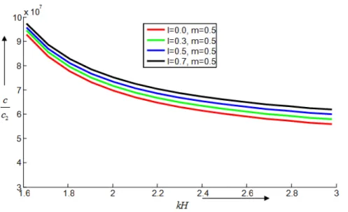
2 0.5 present in the lower half-space. It is clear fromthis figure, the phase velocity increases with increase of inhomogeneity parameters k. Figure 3 represents the variation of dimensionless phase velocity c c2 in intermediate layer against dimensionless wave number kH of Love wave for different values of initial stress parameterP
2
and in the presence of constant inhomogeneity parameter k 0.5 present in the lower half-space. The values of stress parameters for curves have been taken as 0.0, 0.3, 0.5 and 0.7, respectively. It is observed from these curves that as the stress parameters in the half-space increases, the velocity of Love wave increases. Figure 4 shows the effect of initial stress parameters on dimensionless phase velocity c c2 in intermediate layer against dimensionless wave number kH of Love wave in the presence of constant inhomogeneity parameter for homogeneous media. From above numerical analysis, the following observations are made:
i. In entire figures, dimensionless phase velocity c c2 of Love waves in intermediate layer decreases with increase of dimensionless wave number kH .
ii. The dimensionless phase velocity c c2 of Love wave in intermediate layer shows remarkable change with inhomogeneity k and stress parameters P
2
.iii. It is observed as the depth increases the velocity of Love wave in intermediate layer decreases. iv. The phase velocity c c2 of Love wave in intermediate layer decreases with the decrease of
initial stress P
2
of lower half-space.v. The phase velocity c c2 of Love wave in intermediate layer increases with the increase of inhomogeneity parameter k of lower half-space.
Figure 2: Dimensionless phase velocity c c2 in intermediate layer against dimensionless wave number kHof Love wave for different values of inhomogeneity parameter l k and in the presence of constant initial stress
parameter m P
2 0.5 present in the lower half-space.Figure 3: Dimensionless phase velocity c c2 in intermediate layer against dimensionless wave number kHof
Love wave for different values of initial stress parameter mP
2 and in the presence of constant inhomogeneity parameter l k 0.5 present in the lower half-space.7 CONCLUSIONS
In this paper, an analytical approach is used to investigate the propagation of Love wave in a homogeneous isotropic layer of finite thickness between orthotropic and inhomogeneous half spaces. It has been observed that present geometry allows Love waves to propagate. Implicit dispersion relation and closed form solutions for displacement in the layer and half-spaces have been obtained. The significant effect of inhomogeneity parameters and stress parameters on Love wave propagation
Figure 4: Dimensionless phase velocity c c2 in intermediate layer against dimensionless wave number kHof
Love wave for different values of initial stress parameter m P
2 and in the presence of constant inhomogeneity parameter l k for homogeneous media.has been observed. Phase velocity has been also computed numerically, and the effects of variation in density and rigidity in the lower half-space have been studied. It has been investigated that the initial stresses have a pronounced effect on the propagation of Love waves. In special cases, when the intermediate layer and lower half-space or intermediate layer and upper half-space are homogeneous, our computed equation coincides with the classical equation of Love wave. Since Earth is an initially stressed, orthotropic and can be considered as composed of different inhomogeneous layers, hence, it is more realistic to consider the inhomogeneity and initial stress discussed in the present problem to study the propagation of Love waves in prestressed inhomogeneous Earth medium. The present study may be useful for geophysical applications of propagation of Love waves in different layers of Earth.
Acknowledgements
The author thanks the GNA University, for providing the use of facilities for research. The author also expresses his sincere thanks to the honorable reviewers for their useful suggestions and valuable comments.
References
Ahmed, S.M., Abd-Dahab, S.M., (2010). Propagation of Love waves in an orthotropic Granular layer under initial stress overlying a semi-infinite Granular medium. Journal of Vibration and Control 16(12): 1845–1858.
Bhattacharya, J., (1969). The possibility of the propagation of Love waves in an intermediate heterogeneous layer lying between two semi-infinite isotropic homogeneous elastic layers. Pure and Applied Geophysics 72(1): 61–71. Chakraborty, S.K., Dey, S., (1982). The propagation of Love waves in water saturated soil underlain by heterogeneous elastic medium. Acta Mech. 44: 169–176.
Chattaraj, R., Samal, S.K., Mahanti, N.C., (2013). Dispersion of Love wave propagating in irregular anisotropic porous stratum under initial stress. International Journal of Geomechanics 13(4): 402-408.
Chatopadhyay, A., (1975). On the dispersion equation for Love wave due to irregularity in the thickness of non-homogeneous crustal layer. Acta Geo. Pol. 23: 307-317.
Deresiewicz, H., (1962). A note on Love waves in a homogeneous crust overlying an inhomogeneous substratum. Bull. Seis. Soc. Amp. 52: 639–645.
Du, J.K., Xian, K., Wang, J., Yong, Y.K., (2008). Propagation of Love waves in prestressed piezoelectric layered structures loaded with viscous liquid. Acta Mechanica Solida Sinica 21(6): 542-548.
Ewing, W.M., Jardetzky, W.S., Press, F., (1957). Elastic Waves in Layered Media. McGraw-Hill, New York. Ghorai, A.P., Samal, S.K., Mahanti, N.C., (2010). Love waves in a fluid-saturated porous layer under a rigid boundary and lying over an elastic half-space under gravity. Appl. Math. Model 34: 1873–1883.
Gubbins, D., (1990). Seismology and Plate Tectonics. Cambridge: Cambridge University Press.
Gupta, S., Majhi, D.K., Kundu, S., Vishwakarma, S.K., (2013). Propagation of Love waves in non-homogeneous substratum over initially stressed heterogeneous half-space. Applied Mathematics and Mechcanics 34: 249–258. Kadian, P., Singh, J., (2010). Effect of size of barrier on reflection of Love Waves. International Journal of Engineering and Technology 2(6): 458-461.
Kakar, R., Gupta, M., (2014). Love waves in an intermediate heterogeneous layer lying in between homogeneous and inhomogeneous isotropic elastic half-spaces. EJGE 19 (Bund. X): 7165-7185.
Ke, L.L., Wang, Y.S., Zhang, Z.M., (2005). Propagation of Love Waves in an inhomogeneous fluid saturated porous layered half-space with properties varying exponentially. International Journal of Geomechanics 131(12): 1322-1328. Kundu, S., Gupta, S., Majhi, D.K., (2013). Love wave propagation in porous rigid layer lying over an initially stressed half space. Appl. Phys.& Math. 3(2): 140-142.
Kundu, S., Gupta, S., Manna, S., (2014a). Propagation of Love wave in fiber-reinforced medium lying over an initially stressed orthotropic half-space. International Journal for Numerical and Analytical Methods in Geomechanics
Kundu, S., Gupta. S., Manna, S., Dolai, P., (2014b). Propagation of Love wave in fiber-reinforced medium over a nonhomogeneous half-space. International J. of Applied Mechanics 6(5): 1450050. DOI: 10.1142/S1758825114500501. 38(11): 1172–1182. DOI: 10.1002/nag.2254.
Liu, J., Wang, Z.K., (2005). The propagation behavior of Love waves in a functionally graded layered piezoelectric structure. Smart Mat. Struct. 14: 137-146.
Love, A.E.H., (1911). Some Problems of Geo-Dynamics. Cambridge University Press, London, UK. Love, A.E.H., (1944). A Treatise on the Mathematical Theory of Elasticity. Dover Publications, New York. Madan, D.K., Kumar, R., Sikka, J.S., (2014). Love wave propagation in an irregular fluid saturated porous anisotropic layer with rigid boundary. Journal of Applied Sciences Research 10(4): 281-287.
Manna, S., Kundu, S., Gupta, S., (2013). Love wave propagation in a piezoelectric layer overlying in an inhomogeneous elastic half-space. Journal of Vibration and Control. DOI: 1077546313513626.
Midya, G.K., (2004). On Love-type surface waves in homogeneous micropolar elastic media. Int. J. Eng. Sci. 42:1275–1288.
Whittaker, E.T., Watson, G.N., (1990). A Course in Modern Analysis. Cambridge University press, London, UK.