Modeling short wave solar radiation using the JGrass-NewAge System

(1)

GMDD

5, 4355–4393, 2012

Modeling short wave solar radiation using

the JGrass-NewAge system

G. Formetta et al.

Title Page

Abstract Introduction

Conclusions References

Tables Figures

◭ ◮

Back Close

Full Screen / Esc

Printer-friendly Version Interactive Discussion

Discussion

P

a

per

|

Dis

cussion

P

a

per

|

Discussion

P

a

per

|

Discussio

n

P

a

per

|

Geosci. Model Dev. Discuss., 5, 4355–4393, 2012 www.geosci-model-dev-discuss.net/5/4355/2012/ doi:10.5194/gmdd-5-4355-2012

Geoscientific Model Development Discussions

This discussion paper is/has been under review for the journal Geoscientific Model Development (GMD). Please refer to the corresponding final paper in GMD if available.

Modeling short wave solar radiation using

the JGrass-NewAge System

G. Formetta1, R. Rigon1, J. L. Ch ´avez2, and O. David2,3

1

University of Trento, 77 Mesiano St., 38123 Trento, Italy

2

Dept. of Civil and Environmental Engineering, Colorado State University, Fort Collins, CO, USA

3

Agricultural Systems Research Unit, USDA-ARS-NPA-ASRU 2150 Centre Ave., Fort Collins, CO 80526, USA

Received: 23 October 2012 – Accepted: 30 November 2012 – Published: 18 December 2012

Correspondence to: G. Formetta (formetta@ing.unitn.it)

(2)

GMDD

5, 4355–4393, 2012

G. Formetta et al.

Title Page

Tables Figures

◭ ◮

Back Close

Full Screen / Esc

Discussion

P

a

per

|

Dis

cussion

P

a

per

|

Discussion

P

a

per

|

Discussio

n

P

a

per

|

Abstract

This paper presents two new modelling components based on the Object Modelling System v3 for the calculation of the shortwave incident radiation ( ˆRsw↓) on complex

topography settings, and the implementation of several ancillary tools. The first com-ponent, NewAGE-SwRB, accounts for slope, aspect, shadow and the topographical 5

information of the sites, and use suitable parametrisation for obtaining the cloudless ir-radiance. A second component, NewAGE-DEC-MOD’s is implemented to estimate the irradiance reduction due to the presence of clouds, according to three parameterisa-tions. To obtain a working modelling composition, suitable to be compared with ground data at measurement stations, the two components are connected to a Kriging compo-10

nent, and, with the use of a further component NewAGE-V (verification package), the performance of modeled ( ˆRsw↓) is quantitatively evaluated. The two components (and

the various parametrisations they contain) are tested using the data from three basins catchments, and some simple verification test is made to assess the goodness of the methods used. The components are part of a larger system, JGrass-NewAGE, their 15

input and outputs are given as geometrical objects immediately visualisable in a GIS (for instance the companion uDig), and can be used seamlessly with the various mod-elling solutions available in JGrass-NewAGE for the estimation of long wave radiation, evapotranspiration, and snow melting, as well as stand-alone components to just esti-mate shortwave radiation for various uses. The modularity of the approach is shown to 20

be extensible to more accurate physical-statistical studies aimed to assess in deep the components performances and extends spatially their results, without the necessity of recoding any part of the component but just making using of connective scripts.

1 Introduction

Solar radiation at the top of the atmosphere is just function of Sun activity but, in 25

the case of hydrological studies, the solar constant, Isc∼1367 [W m

−2

], is used as

(3)

GMDD

5, 4355–4393, 2012

G. Formetta et al.

Title Page

Tables Figures

◭ ◮

Back Close

Full Screen / Esc

Discussion

P

a

per

|

Dis

cussion

P

a

per

|

Discussion

P

a

per

|

Discussio

n

P

a

per

|

a suitable approximation of the irradiance at the top of the atmosphere. This value rep-resents the maximum irradiance when the solar beam hits orthogonally the Earth, and reduction of irradiance due to latitude and longitude, the day of the year, and the hour, is necessary, and can be easily calculated with the desired approximation, e.g. Iqbal (1983) and Liou (2002).

5

In the absence of clouds, solar radiation arrives at the Earth’s ground surface in two classes. Direct radiation (S↓∗) is that part of the solar beam which arrives at the surface without any interaction with the Earth’s atmosphere. Di_ffuse radiation (d∗↓) is shortwave radiation scattered downwards back to the Earth’s surface after hitting molecules of the atmospheric gases and aerosols. In this paper we will call the sum of 10

S↓∗ andd∗↓, total Shortwave Radiation at the ground (R∗↓sw).

When it is assumed that shortwave radiation hits rugged terrains, geometrical cor-rections can be applied to obtain the theoretical irradiances that hit the tilted terrain surface in absence of the atmosphere before accounting for the attenuations due to scattering. These quantities are therefore very far from the real radiation measured by 15

instruments on the ground for the effects introduced by atmosphere’s scattering, reflec-tions, absorptions (Liou, 2002) and landscape multiple reflecreflec-tions, and will be denoted

S↓,d↓andRsw↓through the paper, which shows an implementation of Corripio (2003)

algorithms.

With the development of modern computing power efficient methods were devel-20

oped to estimate irradiance over vast mountain regions. Those studies were based on the elaboration of digital elevation models (DEMs) from which terrain’s characteris-tics were automatically derived, and used algorithms of various degree of complexity. A long series of studies parametrizeRsw↓since the 1960’ies which are well reviewed in

Duguay (1993). Among many, Dozier and Frew (1990) were the first to used DEMs for 25

(4)

GMDD

5, 4355–4393, 2012

G. Formetta et al.

Title Page

Tables Figures

◭ ◮

Back Close

Full Screen / Esc

Discussion

P

a

per

|

Dis

cussion

P

a

per

|

Discussion

P

a

per

|

Discussio

n

P

a

per

|

to estimate S↓ for a whole basin area; Gubler et al. (2012) tried to assess the in-herent error in the estimation of the short wave incoming solar radiation. The above approaches, were aimed to computational efficiency and simplified parameterisations, and produced several software packages that offer different methodologies, such as SolarFlus (in ArcInfo GIS) (Dubayah and Paul, 1995; Hetrick et al., 1993), Solar An-5

alyst (Fu and Rich, 2000), SRAD (by Moore, 1992, and documented in Wilson and Gallant, 2000), Solei (Mikl ´anek, 1993) or r.sun (Hofierka and Suri, 2002), and often integrate the models in GIS. Our modelling, making treasure of these previous efforts, is also in line with those that tried to respond to the increase demand of modularity and interchangeability in hydrological and biophysical models that have been developed in 10

the last decades. This trend is widespread in industrial software and gained momentum also in scientific research in environmental fields (e.g. Jones et al., 2001; David et al., 2002; Donatelli et al., 2006; Rizzoli et al., 2005).

Finally, our e_ffort, in particular uses the Object Modelling System v.3.0 (David et al., 2002, 2010) components’s framework and seamlessly integrates ion the Spatial Tool-15

box of the uDig GIS, which is based upon OMS3.

This paper introduces and tests model components for the estimation of the di-rect solar radiation which are part of a larger modeling effort called JGrass-NewAGE (Formetta et al., 2011, 2013) with the goal of estimating all the components of the hy-drological cycle for medium to large catchments. Of this goal, short wave radiation is 20

an important part since it is necessary for the estimation of long wave radiation, evapo-transpiration and snow cover evolution. However, the modelling components developed work also stand-alone, for any possible use.

2 The JGrass-NewAGE component for the estimation of the shortwave radiation budget (NewAGE-SwRB)

25

This component, NewAGE-SwRB (or simply SwRB in the following) was built to be able to simulate the direct shortwave radiation budget in multiple points in a landscape,

(5)

GMDD

5, 4355–4393, 2012

G. Formetta et al.

Title Page

Tables Figures

◭ ◮

Back Close

Full Screen / Esc

Discussion

P

a

per

|

Dis

cussion

P

a

per

|

Discussion

P

a

per

|

Discussio

n

P

a

per

|

and to provide inputs to hydrological components independently of their geographical structure (either implementing fully distributed, semi-distributed or lumped concepts). Hence, from a spatial point of view, the output of SwRB can be a raster (the results are provided for each pixel of the computational domain) or vectorial (the results are provided only in some points of the computational domain) according to the the mod-5

eller’s needs, and in Open GIS Consortium standard formats (as GridCoverage and shapefiles, respectively). For the various use, the component was re-used to be able to provide results using a generic hourly, sub-hourly and daily time step, according to the users’ specifications.

While not trivial to obtain, the geometrical elaboration of the radiation that returns the 10

incoming solar radiation on a tilted plane, is given for granted, and estimated accord-ing to the elegant solution provided by Corripio’s algorithms (Corripio, 2002, 2003). Therefore in the following is assumed that the solar constant, Isc has been spatially

corrected to account for the geometry and the position of the landscape underneath, to give a “corrected” solar constant, ˆIsc.

15

2.1 Direct Solar Radiation under cloudless sky conditions

Therefore, the incidentR↓sw, on an arbitrary sloping surface in a point, under cloudless

sky condition is given by Corripio (2002):

R↓sw=C1·Iˆsc·E0·cos(θs)·(Ts+βs)·ψ (1)

in which: 20

(6)

GMDD

5, 4355–4393, 2012

G. Formetta et al.

Title Page

Tables Figures

◭ ◮

Back Close

Full Screen / Esc

Discussion

P

a

per

|

Dis

cussion

P

a

per

|

Discussion

P

a

per

|

Discussio

n

P

a

per

|

– E0[–] is a correction factor related to the Earth’s orbit eccentricity computed

ac-cording to Spencer (1971):

E0=1.00011+0.034221 cos(κ)+0.00128 sin(κ)+0.000719 cos(2κ)

+0.000077 sin(2κ) (2)

κ:=2π·

_N₋

1 365

(3) 5

whereκ is the day angle [rad] and N is the day number of the year (N=1 on 1 January,N=365 on 31 December);

– Ts[–], product of the atmospheric transmittances, is defined as:

Ts:=τr·τ0·τg·τw·τa (4)

10

where the τ functions are the transmittance functions for Rayleigh scattering, ozone, uniformly mixed gases, water vapour and aerosols, respectively. They are computed for each point as defined in the last part of this section.

– βs [m] is a correction factor for increased transmittance with elevation z [m]

de-fined according to Corripio (2002): 15

βs= (

2.2×10−5·zp ifz≤3000 m

2.2×10−5·3000.0 ifz >3000 m (5)

– θs [rad] is the angle between the Sun vector and the surface plane (Corripio,

2003); for a horizontal surfaceθs=θzwhereθzis the zenith angle;

– ψs is the shadows index that accounts for the sun or shadow of the point under

analysis, and is modelled according to Corripio (2003): 20

ψs= (

1 if the point p is in the sun

0 if the point p is in the shadow (6)

(7)

GMDD

5, 4355–4393, 2012

G. Formetta et al.

Title Page

Tables Figures

◭ ◮

Back Close

Full Screen / Esc

Discussion

P

a

per

|

Dis

cussion

P

a

per

|

Discussion

P

a

per

|

Discussio

n

P

a

per

|

The atmospheric transmittances in Eq. (4) are estimated according to Bird and Hul-strom (1981) and Iqbal (1983) to result functions of the atmospheric pressure, the ozone layer thickness, the precipitable water amount, the zenith angle and visibility, which are eventually taken in this paper as fixed values, according to the literature values reported in Table 1.

5

The transmittance function for Rayleigh scatteringτr [–] is estimated as:

τr=exp h

−0.0903·m0.84a ·(1+ma−m1.01a ) i

(7)

wherema[–] is the relative air mass at actual pressure defined as:

ma:=mr·

p

1013.25

(8)

in whichp[mbar] is the local atmospheric pressure,mr [–] relative optical air mass:

10

mr=

1.0

cos(θs)+0.15(93.885−(180/2π)θs)−1.253

(9)

The transmittance by ozoneτo[–] is defined as:

τo=1.0− h

0.1611lozmr(1.0+139.48lozmr)−0.3035

− 0.002715lozmr

1.0+0.044lozmr+0.0003 (lozmr)2 i

(10) 15

whereloz [cm] is the vertical ozone layer thickness, and the coefficients have the

ap-propriate dimensionality ti makeτ0dimensionless.

Transmittance by uniformly mixed gasesτg[–] is modelled as:

τg=exp h

−0.0127·m0.26a i

(8)

GMDD

5, 4355–4393, 2012

G. Formetta et al.

Title Page

Tables Figures

◭ ◮

Back Close

Full Screen / Esc

Discussion

P

a

per

|

Dis

cussion

P

a

per

|

Discussion

P

a

per

|

Discussio

n

P

a

per

|

Transmittance by water vapourτwis estimated as:

τw=1.0−

2.4959w mr

(1.0+79.034w mr)0.6828+6.385w mr

(12)

wherew[cm] is precipitable water in cm calculated according to Prata (1996). Finally, the transmittance by aerosolsτa[–] is evaluated as:

5

τa= h

0.97−1.265·V−0.66im

0.9 a

(13)

where V [km] is the visibility, i.e. an estimation of the visibility extent as in Corripio (2002).

2.2 Diffuse solar radiation under cloudless sky conditions

10

The modelling of the diffuse component of solar radiation,d↓follows Iqbal (1983):

d↓=(d↓r+d↓a+d↓m)·Vs (14)

where d↓r, d↓a and d↓m are the diffuse irradiance components after the first pass

through the atmosphere due to the Rayleigh-scattering, the aerosol-scattering and 15

multiple-reflection, respectively.

The Rayleigh-scattered diffuse irradiance is computed as:

d↓r=

0.79·cos(θz)·Isc·E0·τo·τg·τw·τaa·(1−τr)

2.0·(1.0−ma+m1.02a )

(15)

whereτaa is the transmittance of direct radiation due to aerosol absorptance modelled

20 as:

τaa=1.0−(1−ω0)·(1−ma+m1.06a )·(1.0−τa) (16)

(9)

GMDD

5, 4355–4393, 2012

G. Formetta et al.

Title Page

Tables Figures

◭ ◮

Back Close

Full Screen / Esc

Discussion

P

a

per

|

Dis

cussion

P

a

per

|

Discussion

P

a

per

|

Discussio

n

P

a

per

|

whereω0=0.9 [–] is the single-scattering albedo fraction of incident energy scattered

to total attenuation by aerosols (Hoyt, 1978).

The aerosol-scattered diffuse irradiance component is defined as:

d↓a=

0.79·Isc·cos(θz)·E0·τo·τg·τw·τaa·Fc·(1−τas)

1−ma+m1.02a

(17) 5

whereτas:=τaτ− 1

aa andFcis the fraction of forward scattering to total scattering (Iqbal,

1983,Fs=0.84 if no information about the aerosols are available,).

The diffuse irradiance from multiple reflections between the earth and the atmo-sphere is computed as:

d↓m=

(R↓sw+d↓r+d ↓a)·αg·αa

1.0−αg·αa

(18) 10

whereα_g is the albedo of the ground andα_a is the albedo of the cloudless sky com-puted as:

αa=0.0685+(1.0−Fc)·(1−τas) (19)

15

FinallyVsis the sky view factor, i.e. the fraction of sky visible in a point, computed using

the algorithm presented in Corripio (2002).

2.3 The shortwave radiation correction for cloudy sky, DEC-MOD’s

The radiation components presented in the previous subsections are computed un-der the hypothesis of cloudless sky conditions. To account for the presence of clouds, 20

some models found in the literature were denominated decomposition models. The procedure described here is in line with Helbig et al. (2010). It corrects the clear sky direct and diffuse irradiance by means of adjustment coefficients and the clear sky irradiances so that, for any point:

S↓∗:₌cs·S↓ (20)

(10)

GMDD

5, 4355–4393, 2012

G. Formetta et al.

Title Page

Tables Figures

◭ ◮

Back Close

Full Screen / Esc

Discussion

P

a

per

|

Dis

cussion

P

a

per

|

Discussion

P

a

per

|

Discussio

n

P

a

per

|

is the corrected irradiance for direct shortwave radiation (andcsis the correction

coef-ficient forS↓), and

d↓∗:=cd·d↓ (21)

is the corrected irradiance for the diffuse shortwave radiation (andcdis the correction

coefficient for d↓). The coefficients of reduction are made dependent upon the global 5

shortwave irradiance measured at the available stations as suggested by Orgill and Hollands (1977), Erbs et al. (1982) and Reindl et al. (1990), so that, for any station,i:

ˆ

Rsw↓i=S ↓∗i +d

∗_↓

i (22)

d∗↓i=(kd)iRˆsw↓i (23)

10

equation which also definekd, the ratio between the diffuse shortwave irradiance and

the shortwave total irradiance. Therefore, at stations:

(cd)i=

ˆ

Rsw↓i ·kd

d ↓_i (24)

and

(cs)i =

ˆ

Rsw↓i ·(1−(kd)i)

S↓i

(25) 15

Clearlykdbecomes the key parameter to be determined to close, for the stations, the

estimation of the cloudy irradiances. To this goal, we use here three di_fferent parame-terisations.

– Erbs et al. (1982) estimated kd for latitudes between 31 and 42 degrees North,

using hourly data from five irradiances measurement stations in the USA: 20

kd= 

 

 

1.0−0.09k_t ifk_t≤0.22

0.951−0.1604kt+4.388k 2

t −16.638k 3

t +12.336k 4

t if 0.22< kt≤0.80

0.165 ifkt>0.80

(11)

GMDD

5, 4355–4393, 2012

G. Formetta et al.

Title Page

Tables Figures

◭ ◮

Back Close

Full Screen / Esc

Discussion

P

a

per

|

Dis

cussion

P

a

per

|

Discussion

P

a

per

|

Discussio

n

P

a

per

|

(26)

– Reindl et al. (1990) estimated the diffuse fraction kd knownkt using data

mea-sured in USA and Europe (latitude between 28–60 degrees N) and provided this relations:

kd= 

 

 

1.02−0.248·k_t ifk_t≤0.30

1.45−1.67k_t if 0.30< k_t≤0.78 0.147 ifkt>0.78

(27) 5

– Boland et al. (2001) using data from Victoria, Australia, provided the exponential relation:

kd=

1.0

1.0+e7.997(kt−0.586)

(28)

In turn Eq. (22) above is completely determined by the knowledge of the clearness sky index,kt [–], which is defined as:

10

k_t:= Rˆsw↓

ˆ

Isc·E0·cos(θs)

(29)

Using the above equations a set of adjustment coefficients, cs and cd for beam and

diffuse radiation component are obtained for the measurements station. To be extended to any spatial point, they need to be extrapolated to all the points of interest (where incoming shortwave solar radiation is not measured). This is accomplished in NewAGE-15

(12)

GMDD

5, 4355–4393, 2012

G. Formetta et al.

Title Page

Tables Figures

◭ ◮

Back Close

Full Screen / Esc

Discussion

P

a

per

|

Dis

cussion

P

a

per

|

Discussion

P

a

per

|

Discussio

n

P

a

per

|

3 Applications

The capability of the model was tested by joining with the appropriate OMS script (avail-able in the complementary material) four JGrass-NewAGE components: the SwRB, the (Radiation Decomposition model) DEC-MOD’s, the Kriging and the NewAGE-V (Verifi-cation) package connected as illustrated in Fig. 1.

5

Below we described the basins used for the verification, comments their data, and illustrate the procedure of verification.

3.1 Reference catchments

Three different river basins were used: Little Washita river basin (Oklahoma, US), Fort Cobb river basin (Oklahoma, US) and Piave radiation dataset (Veneto, Italy). As pre-10

sented in the next subsections, di_fferences between the two places in elevation range, number of monitoring points, latitudes, and complexity of the topography are substan-tial.

The Little Washita river basin (611 km2) is located in southwestern Oklahoma, be-tween Chickasha and Lawton and its main hydrological and geological features are 15

presented in Allen and Naney (1991). The elevation range is between 300 and 500 m above sea level, the main land use are range, pasture, forest, cropland. The mean an-nual precipitation is 760 mm and the mean air temperature is 16 degrees Celsius. Sev-enteen meteorological stations of the ARS Micronet (http://ars.mesonet.org/) are used for the simulations and for each stations are available five minutes measurements of: 20

air temperature at a height of 1.5 m, relative humidity at a heigth of 1.5 m and incoming global solar radiation. The data for the year 2002 were summed to an hourly time step to be used in the simulations. The meteorological stations main features are reported in Table 2 and Fig. 5 shows their location.

The Fort Cobb river basin (813 km2) is located in southwestern Oklahoma and an ex-25

haustive description is given in Rogers (2007). The elevation range is between 400 and 570 m above the sea level, the main land usage are cropland, range, pasture, forest,

(13)

GMDD

5, 4355–4393, 2012

G. Formetta et al.

Title Page

Tables Figures

◭ ◮

Back Close

Full Screen / Esc

Discussion

P

a

per

|

Dis

cussion

P

a

per

|

Discussion

P

a

per

|

Discussio

n

P

a

per

|

water. The long record mean annual precipitation is 816 mm and the mean annual air temperature is 18 degrees Celsius. Eight meteorological stations of the ARS Micronet (http://ars.mesonet.org/) are used for the simulations. The data for the year 2006 were accumulated to an hourly time step and used in the simulations.

The meteo stations main features are reported in Table 3 and the top of Fig. 6 shows 5

their position.

The Piave river basin area (3460 km2) is located in the north-eastern part of the Ital-ian peninsula. The elevation range is between 700 and 3160 m above sea level, the main soil uses are: (i) crops up to 500 m a.s.l., (ii) evergreen and deciduous forests at elevation between 500 and 1800 m a.s.l. and (iii) alpine pasture and rocks at higher 10

elevations. The mean annual precipitation is around 1500 mm and the mean air tem-perature is 10◦C.

Seventeen meteorological stations are used for the simulations and for each stations are available five minutes measurements of: air temperature at a heigth of 1.5 m, rela-tive humidity at a heigth of 1.5 m and incoming global solar radiation. The data for the 15

year 2010 were summarized to an hourly time step and were used in the simulations. The meteo stations main features are reported in Table 4 and the top of Fig. 7 shows their position.

3.2 Data analysis

As presented in Tovar et al. (1995), the solar radiation measurement over a flat and 20

homogeneous landscape are well correlated and the correlation decrease with the dis-tances from the considered station. If we move the analysis on the complex topography landscape the correlation between solar radiation measurement decrease respect to the flat landscape. This is confirmed in the analyses datasets. In particular, we focus our attention on the Little Washita river basin, which can be considered a flat and ho-25

(14)

GMDD

5, 4355–4393, 2012

G. Formetta et al.

Title Page

Tables Figures

◭ ◮

Back Close

Full Screen / Esc

Discussion

P

a

per

|

Dis

cussion

P

a

per

|

Discussion

P

a

per

|

Discussio

n

P

a

per

|

top and at the bottom, respectively. For Little Washita river basin the correlogram be-tween measurement stations shows high values through the whole basin. The Piave river basin is much more rugged and its correlogram, in agreement with other literature findings (e.g. Tovar et al., 1995; Long and Ackerman, 1995), is much lower. Moreover the correlogram on Piave river basin decreases faster than the correlogram on Lit-5

tle Washita river basin, and this certainly would imply a minor predictive capability of quantities based on measurements statistics.

3.3 Plan of simulations and verification method

The SwRB component just estimate for any point of a basin the incoming radiation. It does not require any calibration, once the four parameters in Table 1 are assigned 10

according to literature values. These outputs, however, do not correspond to a mea-sured quantity but to an intermediate step of the calculations. Just the data coming out from the DEC-MOD’s component correspond to measured quantities, and, actually, this component uses the measured quantity to estimate the attenuation coefficients. There-fore to allow some validation, we divided any of the group of measurements stations 15

into two subgroup: one used for the estimation of the coefficients, (say C-set), and the other for the verification of the results, (say V-set). Stations used for verification are in bold letters in Tables 2, 3 and 4. More complex verification strategies could be used, as described in the discussion section, but their application is beyond the scope of the present work.

20

Therefore, for any of the three basins is applied:

– the SwRB in the subset of the measurement stations. The result for this step is the computation of the clear sky surface shortwave radiation. Inputs and outputs of the model are reported in Table 1. The main parameters value used in the simulations are reported in Table 1 according to Iqbal (1983) and Corripio (2002); 25

– the DEC-MOD’s presented in the previous section and estimation of the coeffi -cientscsandcd. Inputs and outputs of the model are reported in Fig. 1;

(15)

GMDD

5, 4355–4393, 2012

G. Formetta et al.

Title Page

Tables Figures

◭ ◮

Back Close

Full Screen / Esc

Discussion

P

a

per

|

Dis

cussion

P

a

per

|

Discussion

P

a

per

|

Discussio

n

P

a

per

|

– the ordinary Kriging component (Formetta et al., 2011) to extrapolate the coeffi -cientscs and cd for the set of stations left for verification (in bold in Tables 2, 3

and 4);

– an estimate of the shortwave incoming solar radiation under generic sky condi-tion in the V-set (SwRB-Allsky, which multiply the SwRB output by the correccondi-tion 5

coefficients kriging output for the V-Set stations);

– the verification component NewAGE-V (Formetta et al., 2011) to evaluate the per-formance of the model.

For the simulations of this paper, the Erbs model was used in the case of Piave river basin and Reindl model was used for Little Washita and Fort Cobb catch-10

ments.

For verification we used three index of performances:

– mean absolute error (MAE):

MAE= 1

N ·

N X

i

|S_i−O_i| (30)

whereN is the number of records of the time-series, Oare the observed values 15

andS are the simulated values. MAE is expressed in the same units ofOandS, and is zero for perfect agreement between observations and estimates.

– Percentual bias (PBIAS):

PBIAS=100·

PN

i (Si−Oi)

PN

i Oi

(31)

PBIAS measures the average tendency of the simulated values to be larger or 20

(16)

GMDD

5, 4355–4393, 2012

G. Formetta et al.

Title Page

Tables Figures

◭ ◮

Back Close

Full Screen / Esc

Discussion

P

a

per

|

Dis

cussion

P

a

per

|

Discussion

P

a

per

|

Discussio

n

P

a

per

|

– Kling Gupta Efficiency (KGE) as reported in Gupta et al. (2009):

KGE=1− q

(R−1)2₊₍_A₋₁₎2₊₍_B₋₁₎2 ₍₃₂₎

in whichRrepresents the linear correlation coefficient between the simulated (S) and measured (O) values,Aand B are, respectively expressed in Eqs. (21) and 5

(22):

A=σ_σo s

(33)

whereσo is the observed standard deviation value andσs is the simulated

stan-dard deviation value; 10

B=µs−µo

σo

(34)

whereµs and µo are the means of simulated (S) and measured (O) values. For

this index, the best agreement is obtained with the value 1.

The Kriging package can utilise the most common variogram models (spheric, 15

linear, exponential, gaussian). However, for these cases below, a linear model was used.

3.4 Results

Results are analysed separately for the three case studies. They confirm the results found in the literature, and reveal a reasonable agreement between measured and 20

simulated data.

3.4.1 Results for Little Washita river basin

Figure 5 shows the scatter plot between the modelled and the measured total incoming solar radiation in the four stations of the V-set.

(17)

GMDD

5, 4355–4393, 2012

G. Formetta et al.

Title Page

Tables Figures

◭ ◮

Back Close

Full Screen / Esc

Discussion

P

a

per

|

Dis

cussion

P

a

per

|

Discussion

P

a

per

|

Discussio

n

P

a

per

|

Table 5 shows the result of the NewAge-V which accepts in input measured and modelled time series and provides as output the user defined goodness of fit indexes.

3.4.2 Results for Fort Cobb river basin

For the Fort Cobb river, the same procedure presented for the Little Washita river basin was followed.

5

Figure 6 shows the scatter plot between the modelled and the measured total in-coming solar radiation in the four V-set stations. Table 6 show the results in term of goodness of fit indices for the V-set.

3.4.3 Results for Piave river basin

For the Arabba river is repeated the same procedure presented for the Little Washita 10

river basin. The decomposition model used in this case is Reindl et al. (1990). Figure 7 shows the scatter plot between the modelled and the measured total incoming solar radiation in the four V-set. Table 7 show the results in term of goodness of fit indexes for the same set of stations.

4 Discussion

15

4.1 About SwRB and DRM components’ predictive capabilities

The model applications are performed in case studies where topography has different characteristics: (a) two cases presented gentle topography and high density measure-ment network (for the experimeasure-mental Little Washita and Fort Cobb watersheds) (b) the other case presented a typical case of hydrological basin with complex topography, 20

(18)

GMDD

5, 4355–4393, 2012

G. Formetta et al.

Title Page

Tables Figures

◭ ◮

Back Close

Full Screen / Esc

Discussion

P

a

per

|

Dis

cussion

P

a

per

|

Discussion

P

a

per

|

Discussio

n

P

a

per

|

In all the cases the model was able to simulate the global shortwave solar radiation showing relatively good goodness of fit indices presented in Tables 5 and 6 for Little Washita and Fort Cobb, respectively and in Table 7 for the Arabba river basin.

The model performs with the similar and acceptable accuracy both for Little Washita and Fort Cobb river basin. The result is confirmed by the goodness of fit indices and 5

by the graphical analysis.

The model performance deteriorated in the Arabba case study. This could be due to the effect of the complex topography on the computation of the clear sky solar radiation but also to the lower measurements stations density in high elevation zones.

Because of this topographic condition the increasing measurement data uncertainty 10

about the temperature and humidity influenced the atmospheric transmittance compu-tations. This is confirmed also by the data analysis: for the Piave river basin ments shows lower correlation respect, for example, the correlation between measure-ments on the Little Washita river basin, where the gentle topography does not play a crucial rule.

15

Regardless, the model, also in the case of complex topography watershed was able to reproduce well the shortwave solar radiation. The PBIAS index was equal to 14.80 in the worst case. According the hydrological model classification based on PBIAS index, presented in Van Liew et al. (2005) and Stehr et al. (2008), the results achieved in our study are classified as “good” and therefore the solar radiation model is suitable to be 20

used to estimate incoming shortwave solar radiation.

4.2 About the possibilities open by the components’ structure of JGrass-NewAGE

Since the goal of the paper was to show how the components work, the statistical analysis of the results was maintained to a simple level. One more accurate procedure 25

of testing of the components performances would be to apply a “Jack-knife” procedure to estimate errors (as proposed by Quenouille, 1956; Miller, 1974). In this procedure, the V-set, would vary among all the stations and an overall statics could be delineated.

(19)

GMDD

5, 4355–4393, 2012

G. Formetta et al.

Title Page

Tables Figures

◭ ◮

Back Close

Full Screen / Esc

Discussion

P

a

per

|

Dis

cussion

P

a

per

|

Discussion

P

a

per

|

Discussio

n

P

a

per

|

According to Tovar et al. (1995) and Long and Ackerman (1995) studies, the influ-ence of the aspect of the measurements station could have been identified. This opera-tion and analysis, indeed time consuming, can be made, simply by adding a Jack-Knife component to the structure of the model at “linking time”, i.e. using the script that con-nects the components. As presented in Fig. 3, by using the encapsulation properties 5

of OMS, no modification of the core components is needed to accomplish this task. Other components, in the set of the New-AGE system (e.g. Formetta et al., 2011), allow to perform parameter calibration. In this paper no calibration was performed of the four parameter (in Table 1) needed to run the SwRB component. However, it can be easily envisioned, the use of, for instance, the particle swarm NewAge component 10

(Formetta et al., 2011) for automatic calibration. In this case the diagram of linked components would be the one shown in Fig. 4.

Eventually, the four parameters can become variable in space, and, in this case, would become reasonable to use the Kriging spatial interpolators to give their spatial structure. This would allow for studying the spatial variability of radiative transmittance 15

with position or other characteristics as height, aspect and slope of the terrain.

All of these simulations (Formetta et al., 2013) do not require any rewriting of the code, except the adjustment of the scripts to execute them. At each addition of com-plexity, derived from adding a component or making spatial a parameter set, the im-provement on the final results can be objectively determined with the use of the good-20

ness of fit component, and the user can objectively judge if, with the present parame-terisations, the introduction of complexities is worthwhile.

5 Conclusions

The goal of this paper was to present a set of hydrological components to estimate the shortwave incoming solar radiation present in the JGrass-NewAGE system. These 25

(20)

GMDD

5, 4355–4393, 2012

G. Formetta et al.

Title Page

Tables Figures

◭ ◮

Back Close

Full Screen / Esc

Discussion

P

a

per

|

Dis

cussion

P

a

per

|

Discussion

P

a

per

|

Discussio

n

P

a

per

|

object oriented features that make possible a flexible modelling structure apt to inves-tigate many scientific questions with a minimum of e_ffort.

The core components presented cover: the simulation of the incoming shortwave radiation under cloudless conditions, and the estimation of the effects of clouds with three di_fferent parametrisation of the irradiance reduction. Main ancillary components 5

used in the paper are the JGrass-V and the Kriging components, used, respectively for the verification of the results, and the spatial interpolation of irradiance reduction characteristics.

The outputs provided by the model composition shown are independent of both the simulation time step and of the spatial resolution the user want to use. This mean 10

that they can be integrated in both semi-distributed hydrological model and for fully distributed hydrological model (once these models follow the conditions required by OMS3).

The theoretical formulation of the model composition used in the paper is tested by using three datasets from different watersheds (different geomorphological and clima-15

tological features) with good results as quantified by some objective indexes.

The model, as made by OMS3 components is able to use all of the Jgrass-NewAge components such as the GIS visualization tools inherited from uDig (http: //udig.refractions.net), and being connected to other components, for calibration of the parameters, estimation of long wave radiation, evapotranspiration and discharge, and 20

for snow modelling, as presented in Formetta et al. (2011).

Further the paper shows some possibility offered by the modelling by components paradigm in envisioning various possible analyses obtained by the composition of dif-ferent modelling components in the pool of the ones of the JGrass-NewAGE system.

If another parameterisation of the same radiation processes will be introduced in 25

the future, it will simply constitute an alternative component that that could be inserted by adding or eliminating it from the simulation script just before the run-time, without altering any other piece of the modelling solution.

(21)

GMDD

5, 4355–4393, 2012

G. Formetta et al.

Title Page

Tables Figures

◭ ◮

Back Close

Full Screen / Esc

Discussion

P

a

per

|

Dis

cussion

P

a

per

|

Discussion

P

a

per

|

Discussio

n

P

a

per

|

Acknowledgement. This paper has been partially produced with financial support from the Hy-droAlp project, financed by the Province of Bolzano. The Authors thanks Andrea Antonello and Silvia Franceschi (Hydrologis) and Daniele Andreis for their work on preliminary versions of parts of the codes.

References

5

Allen, P. and Naney, J.: Hydrology of the Little Washita River Watershed, Oklahoma: Data and Analyses. USDA-ARS, ARS-90. December, 1991. 4366

Bird, R. and Hulstrom, R.: Simplified clear sky model for direct and diffuse insolation on hori-zontal surfaces, Tech. rep., Solar Energy Research Inst., Golden, CO (USA), 1981. 4361 Boland, J., Scott, L., and Luther, M.: Modelling the diffuse fraction of global solar radiation on

10

a horizontal surface, Environmetrics, 12, 103–116, 2001. 4365

Corripio, J.: Modelling the energy balance of high altitude glacierised basins in the Central Andes., Ph.D. dissertation, University of Edinburgh, 2002. 4359, 4360, 4362, 4363, 4368, 4379

Corripio, J.: Vectorial algebra algorithms for calculating terrain parameters from DEMs and solar

15

radiation modelling in mountainous terrain, Int. J. Geogr. Inf. Sci., 17, 1–24, 2003. 4357, 4359, 4360

David, O., Markstrom, S., Rojas, K., Ahuja, L., and Schneider, I.: The object modeling system. Agricultural system models in field research and technology transfer, Press LLC, Chapter 15, 317- 333, 2002. 4358

20

David, O., Ascough, J., Leavesley, G., and Ahuja, L.: Rethinking modeling framework design: object modeling system 3.0, in: IEMSS 2010 International Congress on Environmental Mod-eling and Software ModMod-eling for Environments Sake, Fifth Biennial Meeting, July 5–8, 2010, Ottawa, Canada; Swayne, Yang, Voinov, Rizzoli, and Filatova (Eds.), 1183–1191, 2010. 4358 Donatelli, M., Carlini, L., and Bellocchi, G.: A software component for estimating solar radiation,

25

Environ. Model. Softw., 21, 411–416, 2006. 4358

Dozier, J. and Frew, J.: Rapid calculation of terrain parameters for radiation modeling from digital elevation data, IEEE T. Geosci. Remote, 28, 963–969, 1990. 4357

Dubayah, R.: Modeling a solar radiation topoclimatology for the Rio Grande River Basin, J. Veg. Sci., 5, 627–640, 1994. 4357

(22)

GMDD

5, 4355–4393, 2012

G. Formetta et al.

Title Page

Tables Figures

◭ ◮

Back Close

Full Screen / Esc

Discussion

P

a

per

|

Dis

cussion

P

a

per

|

Discussion

P

a

per

|

Discussio

n

P

a

per

|

Dubayah, R. and Paul, M.: Topographic solar radiation models for GIS, Int. J. Geogr. Inf. Sys., 9, 405–419, 1995. 4358

Duguay, C.: Radiation modeling in mountainous terrain review and status, Mountain Research and Development, 13, 339–357, 1993. 4357

Erbs, D., Klein, S., and Duffie, J.: Estimation of the diffuse radiation fraction for hourly, daily and

5

monthly-average global radiation, Solar Energy, 28, 293–302, 1982. 4364

Formetta, G., Mantilla, R., Franceschi, S., Antonello, A., and Rigon, R.: The JGrass-NewAge system for forecasting and managing the hydrological budgets at the basin scale: models of flow generation and propagation/routing, Geosci. Model Dev., 4, 943–955, doi:10.5194/gmd-4-943-2011, 2011. 4358, 4365, 4369, 4373, 4374

10

Formetta, G., Chavez, J., David, O., and Rigon, R.: Shortwave radiation variability on complex terrain., in preparation, Geosci. Model Dev., 2013. 4358, 4373

Fu, P. and Rich, P.: The solar analyst 1.0 user manual, Helios Environmental Modeling Institute, 1616 Vermont St KS, 66044 USA, 2000. 4358

Goovaerts, P.: Geostatistics for Natural Resources Evaluation, Oxford University Press, USA,

15

1997. 4365

Gubler, S., Gruber, S., and Purves, R. S.: Uncertainties of parameterized surface downward clear-sky shortwave and all-sky longwave radiation., Atmos. Chem. Phys., 12, 5077–5098, doi:10.5194/acp-12-5077-2012, 2012. 4358

Gupta, H., Kling, H., Yilmaz, K., and Martinez, G.: Decomposition of the mean squared error

20

and NSE performance criteria: implications for improving hydrological modelling, J. Hydrol., 377, 80–91, 2009. 4370

Helbig, N., L ¨owe, H., Mayer, B., and Lehning, M.: Explicit validation of a surface shortwave radiation balance model over snow-covered complex terrain, J. Geophys. Res.-Atmos., 115, D18113, 2010. 4363

25

Hetrick, W., Rich, P., Barnes, F., and Weiss, S.: GIS-based solar radiation flux models, in: ACSM ASPRS Annual Convention, 3, 132–132, American Soc. Photogr. Remote Sens. +Amer. Cong. on Bethesda, Maryland, 1993. 4358

Hofierka, J. and Suri, M.: The solar radiation model for Open source GIS: implementation and applications, Proceedings of the Open source GIS – GRASS users conference 2002 – Trento,

30

Italy, 11–13 September 2002. 4358

Hoyt, D.: A model for the calculation of solar global insolation, Solar Energy, 21, 27–35, 1978. 4363

(23)

GMDD

5, 4355–4393, 2012

G. Formetta et al.

Title Page

Tables Figures

◭ ◮

Back Close

Full Screen / Esc

Discussion

P

a

per

|

Dis

cussion

P

a

per

|

Discussion

P

a

per

|

Discussio

n

P

a

per

|

Iqbal, M.: An Introduction to Solar Radiation, 1983. Academic Press, Orlando, FL, USA. 4357, 4361, 4362, 4363, 4368

Jones, J., Keating, B., and Porter, C.: Approaches to modular model development, Agric. Sys., 70, 421–443, 2001. 4358

Liou, K.: An Introduction to Atmospheric Radiation, 84, Academic Press USA, 2002. 4357

5

Long, C. N. and Ackerman, T. P.: Surface Measurements of Solar Irradiance: A Study of the Spatial Correlation between Simultaneous Measurements at Separated Sites, J. Appl. Me-teorol., 34, 1039–1046, doi:10.1175/1520-0450(1995)034<1039:SMOSIA>2.0.CO;2, 1995. 4368, 4373

Mikl ´anek, P.: The estimation of energy income in grid points over the basin using simple digital

10

elevation model, in: Ann. Geophys., 11, European Geophysical Society, Springer, 1993. 4358 Miller, R.: The jackknife – a review, Biometrika, 61, 1–15, 1974. 4372

Moore, I.: SRAD: direct, di_ffuse, reflected short wave radiation, and the e_ffects of topographic shading. Terrain Analysis Programs for Environmental Sciences (TAPES) Radiation Program Documentation, Center for Resource and Environmental Studies, Australia National

Univer-15

sity, Canberra, Australia, 1992. 4358

Orgill, J. and Hollands, K.: Correlation equation for hourly diffuse radiation on a horizontal surface, Solar Energy, 19, 357–359, 1977. 4364

Prata, A.: A new long-wave formula for estimating downward clear-sky radiation at the surface, Q. J. Roy. Meteorol. Soc., 122, 1127–1151, 1996. 4362

20

Quenouille, M.: Notes on bias in estimation, Biometrika, 43, 353–360, 1956. 4372

Ranzi, R. and Rosso, R.: Distributed estimation of incoming direct solar radiation over a drainage basin, J. Hydrol., 166, 461–478, 1995. 4357

Reindl, D., Beckman, W., and Duffie, J.: Diffuse fraction correlations, Solar Energy, 45, 1–7, 1990. 4364, 4365, 4371

25

Rizzoli, A., Svensson, M., Rowe, E., Donatelli, M., Muetzelfeldt, R., Wal, T., Evert, F., and Villa, F.: Modelling framework (SeamFrame) requirements, Report No. 6, SEAMLESS inte-grated project, EU 6th Framework Programme, contract no. 010036-2, www.SEAMLESS-IP. org, 49 pp., ISBN 90-8585-034-7. 2005. 4358

Rogers, J.: Environmental and water resources: milestones in engineering history: 15–19 May

30

2007, Amer. Society of Civil Engineers, Tampa, Florida, 2007. 4366

(24)

GMDD

5, 4355–4393, 2012

G. Formetta et al.

Title Page

Tables Figures

◭ ◮

Back Close

Full Screen / Esc

Discussion

P

a

per

|

Dis

cussion

P

a

per

|

Discussion

P

a

per

|

Discussio

n

P

a

per

|

Stehr, A., Debels, P., Romero, F., and Alcayaga, H.: Hydrological modelling with SWAT under conditions of limited data availability: evaluation of results from a Chilean case study, Hydrol. Sci. J., 53, 588–601, 2008. 4372

Tovar, J., Olmo, F., and Alados-Arboledas, L.: Local-scale variability of solar radiation in a moun-tainous region, J. Appl. Meteorol., 34, 2316–2328, 1995. 4367, 4368, 4373

5

Van Liew, M., Arnold, J., and Bosch, D.: Problems and potential of autocalibrating a hydrologic model, Trans. ASAE, 48, 1025–1040, 2005. 4372

Wilson, J. and Gallant, J.: Terrain Analysis: Principles and Applications, Wiley, New York, 2000. 4358

(25)

GMDD

5, 4355–4393, 2012

G. Formetta et al.

Title Page

Tables Figures

◭ ◮

Back Close

Full Screen / Esc

Discussion

P

a

per

|

Dis

cussion

P

a

per

|

Discussion

P

a

per

|

Discussio

n

P

a

per

|

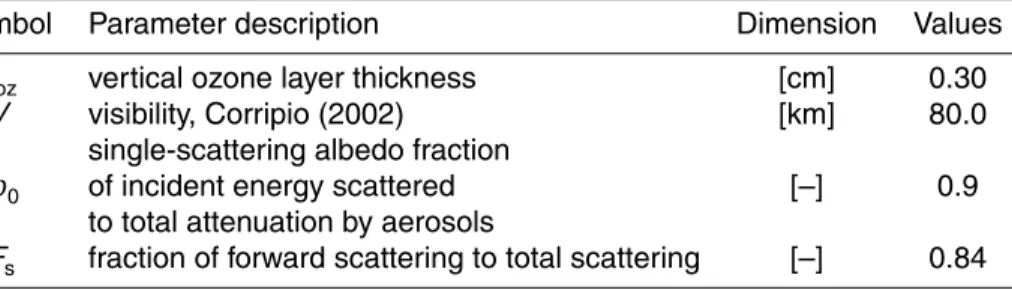
Table 1.List of the SwRB component parameter used in simulations.

Symbol Parameter description Dimension Values

l_oz vertical ozone layer thickness [cm] 0.30

V visibility, Corripio (2002) [km] 80.0

single-scattering albedo fraction

ω₀ of incident energy scattered [–] 0.9

to total attenuation by aerosols

(26)

GMDD

5, 4355–4393, 2012

G. Formetta et al.

Title Page

Tables Figures

◭ ◮

Back Close

Full Screen / Esc

Discussion

P

a

per

|

Dis

cussion

P

a

per

|

Discussion

P

a

per

|

Discussio

n

P

a

per

|

Table 2.List of the meteorological stations used in the simulations performed on Little Washita

river basin. ID is the station identificative number, City is the closer city to the station, LAT and LONG stand for latitude and longitude, respectively, Elevation and Aspect are the station elevation and aspect, respectively. Bold font is used for indicating the stations belonging to the validation set.

ID City LAT. LONG. Elevation (m) Aspect (◦)

124 Norge 34.9728 –98.0581 387.0 138◦

131 Cyril 34.9503 –98.2336 458.0 245◦

133 Cement 34.9492 –98.1281 430.0 116◦

134 Cement 34.9367 –98.0753 384.0 65◦

135 Cement 34.9272 –98.0197 366.0 182◦

136 Ninnekah 34.9278 –97.9656 343.0 270◦

144 Agawam 34.8789 –97.9172 388.0 50◦

146 Agawam 34.8853 –98.0231 358.0 212◦

148 Cement 34.8992 –98.1281 431.0 160◦

149 Cyril 34.8983 –98.1808 420.0 205◦

150 Cyril 34.9061 –98.2511 431.0 195◦

153 Cyril 34.8553 –98.2121 414.0 165◦

154 Cyril 34.8553 –98.1369 393.0 175◦

156 Agawam 34.8431 –97.9583 397.0 290◦

159 Rush Springs 34.7967 –97.9933 439.0 235◦

162 Sterling 34.8075 –98.1414 405.0 15◦

182 Cement 34.845 –98.0731 370.0 245◦

(27)

GMDD

5, 4355–4393, 2012

G. Formetta et al.

Title Page

Tables Figures

◭ ◮

Back Close

Full Screen / Esc

Discussion

P

a

per

|

Dis

cussion

P

a

per

|

Discussion

P

a

per

|

Discussio

n

P

a

per

|

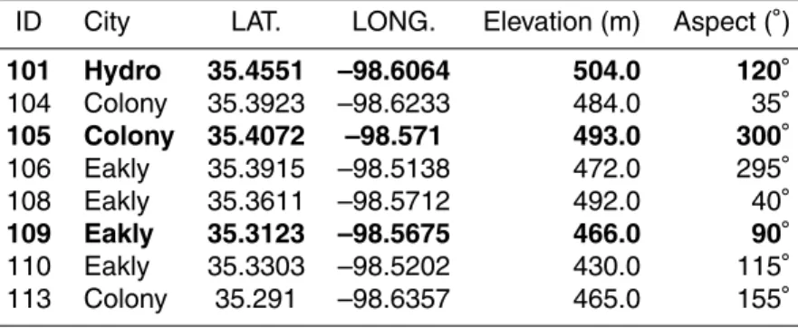
Table 3.List of the meteorological stations used in the simulations performed on Fort Cobb river

basin. ID is the station identificative number, City is the closer city to the station, LAT and LONG stand for latitude and longitude, respectively, Elevation and Aspect are the station elevation and aspect, respectively. Bold font is used for indicating the stations belonging to the validation set.

101 Hydro 35.4551 –98.6064 504.0 120◦

104 Colony 35.3923 –98.6233 484.0 35◦

105 Colony 35.4072 –98.571 493.0 300◦

106 Eakly 35.3915 –98.5138 472.0 295◦

108 Eakly 35.3611 –98.5712 492.0 40◦

109 Eakly 35.3123 –98.5675 466.0 90◦

110 Eakly 35.3303 –98.5202 430.0 115◦

(28)

GMDD

5, 4355–4393, 2012

G. Formetta et al.

Title Page

Tables Figures

◭ ◮

Back Close

Full Screen / Esc

Discussion

P

a

per

|

Dis

cussion

P

a

per

|

Discussion

P

a

per

|

Discussio

n

P

a

per

|

Table 4.List of the meteorological stations used in the simulations performed on Arabba river

basin. ID is the station identificative number, City is the closer city to the station, LAT and LONG stand for latitude and longitude, respectively, Elevation and Aspect are the station elevation and aspect, respectively. Bold font is used for indicating the stations belonging to the validation set.

1 Arabba 46.4999 11.8761 1825 180◦

2 Caprile 46.4404 11.9900 1025 170◦

3 Agordo 46.2780 12.0331 602 5◦

8 Villanova 46.4433 12.2062 972 71◦

9 Auronzo 46.5562 12.4258 940 223◦

11 Campo di Zoldo 46.3466 12.1841 915 160◦

12 Domegge di Cadore 46.4609 12.4103 802 148◦

14 Monte Avena 46.0321 11.8271 761 55◦

18 Passo Pordoi 46.4834 11.8224 357 55◦

21 Passo Monte Croce 46.6521 12.4239 1612 120◦

22 Col Indes 46.1191 12.4401 1119 210◦

23 Torch 46.1515 12.3629 602 177◦

26 Sappada 46.5706 12.7080 1275 156◦

29 Feltre 46.0162 11.8946 273 190◦

31 Falcade 46.3554 11.8694 1151 50◦

32 Cortina 46.536 12.1273 1244 88◦

35 Belluno 46.1643 12.2450 378 157◦

(29)

GMDD

5, 4355–4393, 2012

G. Formetta et al.

Title Page

Tables Figures

◭ ◮

Back Close

Full Screen / Esc

Discussion

P

a

per

|

Dis

cussion

P

a

per

|

Discussion

P

a

per

|

Discussio

n

P

a

per

|

Table 5. Index of goodness of fit between modelled and measured solar radiation on Little

Washita river basin.

STATION ID KGE MAE [W m−2] PBIAS [%]

148 0.94 16.65 4.90

124 0.95 17.50 3.80

182 0.98 16.50 1.80

(30)

GMDD

5, 4355–4393, 2012

G. Formetta et al.

Title Page

Tables Figures

◭ ◮

Back Close

Full Screen / Esc

Discussion

P

a

per

|

Dis

cussion

P

a

per

|

Discussion

P

a

per

|

Discussio

n

P

a

per

|

Table 6.Index of goodness of fit between modelled and measured solar radiation on Fort Cobb

river basin.

STATION ID KGE MAE [W m−2] PBIAS [%]

101 0.96 15.6 5.5

105 0.95 13.50 2.80

109 0.97 14.07 2.70

(31)

GMDD

5, 4355–4393, 2012

G. Formetta et al.

Title Page

Tables Figures

◭ ◮

Back Close

Full Screen / Esc

Discussion

P

a

per

|

Dis

cussion

P

a

per

|

Discussion

P

a

per

|

Discussio

n

P

a

per

|

Table 7.Index of goodness of fit between modelled and measured solar radiation on Arabba

river basin.

STATION ID KGE MAE PBIAS

2 0.92 4.53 2.7

9 0.89 22.10 14.80

(32)

GMDD

5, 4355–4393, 2012

G. Formetta et al.

Title Page

Tables Figures

◭ ◮

Back Close

Full Screen / Esc

Discussion

P

a

per

|

Dis

cussion

P

a

per

|

Discussion

P

a

per

|

Discussio

n

P

a

per

|

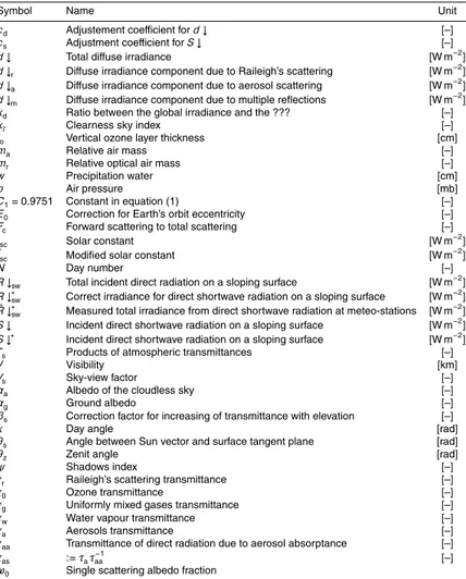
Table 8.List of symbols.

Symbol Name Unit

cd Adjustement coefficient ford↓ [–]

cs Adjustment coefficient forS↓ [–]

d↓ Total diffuse irradiance [W m−2]

d↓r Diffuse irradiance component due to Raileigh’s scattering [W m −2_] d↓a Diffuse irradiance component due to aerosol scattering [W m−2] d↓m Diffuse irradiance component due to multiple reflections [W m−2]

kd Ratio between the global irradiance and the ??? [–]

kt Clearness sky index [–]

lo Vertical ozone layer thickness [cm]

ma Relative air mass [–]

mr Relative optical air mass [–]

w Precipitation water [cm]

p Air pressure [mb]

C1=0.9751 Constant in equation (1) [–]

E0 Correction for Earth’s orbit eccentricity [–]

Fc Forward scattering to total scattering [–]

Isc Solar constant [W m

−2_]

ˆ

Isc Modified solar constant [W m−2]

N Day number [–]

R↓sw Total incident direct radiation on a sloping surface [W m −2_] R↓∗

sw Correct irradiance for direct shortwave radiation on a sloping surface [W m−2]

ˆ

R↓∗

sw Measured total irradiance from direct shortwave radiation at meteo-stations [W m−2] S↓ Incident direct shortwave radiation on a sloping surface [W m−2]

S↓∗ Incident direct shortwave radiation on a sloping surface [W m−2]

Ts Products of atmospheric transmittances [–]

V Visibility [km]

Vs Sky-view factor [–]

αa Albedo of the cloudless sky [–]

αg Ground albedo [–]

βs Correction factor for increasing of transmittance with elevation [–]

κ Day angle [rad]

θs Angle between Sun vector and surface tangent plane [rad]

θz Zenit angle [rad]

ψ Shadows index [–]

τr Raileigh’s scattering transmittance [–]

τ0 Ozone transmittance [–]

τg Uniformly mixed gases transmittance [–]

τw Water vapour transmittance [–]

τa Aerosols transmittance [–]

τaa Transmittance of direct radiation due to aerosol absorptance [–]

τas :=τaτ

−1

aa [–]

ω0 Single scattering albedo fraction

(33)

GMDD

5, 4355–4393, 2012

G. Formetta et al.

Title Page

Tables Figures

◭ ◮

Back Close

Full Screen / Esc

Discussion

P

a

per

|

Dis

cussion

P

a

per

|

Discussion

P

a

per

|

Discussio

n

P

a

per

|

Fig. 1.OMS3 SWRB components of JGrass-NewAge and flowchart to model shortwave

(34)

GMDD

5, 4355–4393, 2012

G. Formetta et al.

Title Page

Tables Figures

◭ ◮

Back Close

Full Screen / Esc

Discussion

P

a

per

|

Dis

cussion

P

a

per

|

Discussion

P

a

per

|

Discussio

n

P

a

per

|

Fig. 2.Correlogram between station 146 and 159 and station on Little Washita river basin, at

the top. Correlogram for station 21 and 26 on Piave river basin, at the bottom.