www.hydrol-earth-syst-sci.net/18/389/2014/ doi:10.5194/hess-18-389-2014
© Author(s) 2014. CC Attribution 3.0 License.
Hydrology and
Earth System
Sciences
Separating the effects of changes in land cover and climate: a
hydro-meteorological analysis of the past 60 yr in Saxony, Germany
M. Renner1,4, K. Brust1, K. Schwärzel2,*, M. Volk3, and C. Bernhofer1
1Technische Universität Dresden, Faculty of Environmental Sciences, Institute of Hydrology and Meteorology,
Chair of Meteorology, Tharandt, Germany
2Technische Universität Dresden, Faculty of Environmental Sciences, Institute of Soil Science and Site Ecology,
Chair of Site Ecology and Plant Nutrition, Tharandt, Germany
3UFZ – Helmholtz Centre for Environmental Research, Department of Computational Landscape Ecology, Leipzig, Germany 4Max-Planck Institute for Biogeochemistry, Biospheric Theory and Modelling Group, Jena, Germany
*now at: United Nations University, Institute for Integrated Management of Material Fluxes and of Resources,
Dresden, Germany
Correspondence to: M. Renner ([email protected])
Received: 14 June 2013 – Published in Hydrol. Earth Syst. Sci. Discuss.: 2 July 2013 Revised: 11 October 2013 – Accepted: 18 December 2013 – Published: 31 January 2014
Abstract. Understanding and quantifying the impact of
changes in climate and land use/land cover on water avail-ability is a prerequisite to adapt water management; yet, it can be difficult to separate the effects of these different im-pacts. In this paper we illustrate a separation and attribu-tion method based on a Budyko framework. We assume that evapotranspiration (ET) is limited by the climatic forcing of
precipitation (P) and evaporative demand (E0), but
modi-fied by land-surface properties. Impacts of changes in climate (i.e.,E0/P) or land-surface changes onETalter the two
di-mensionless measures describing relative water (ET/P) and
energy partitioning (ET/E0), which allows us to separate
and quantify these impacts. We use the separation method to quantify the role of environmental factors onET using
68 small to medium range river basins covering the greatest part of the German Federal State of Saxony within the pe-riod of 1950–2009. The region can be considered as a typical central European landscape with considerable anthropogenic impacts. In the long term, most basins are found to follow the Budyko curve which we interpret as a result of the strong interactions of climate, soils and vegetation. However, two groups of basins deviate. Agriculturally dominated basins at lower altitudes exceed the Budyko curve while a set of high altitude, forested basins fall well below. When visualizing the decadal dynamics on the relative partitioning of water and energy the impacts of climatic and land-surface changes
become apparent. After 1960 higher forested basins experi-enced large land-surface changes which show that the air pol-lution driven tree damages have led to a decline of annualET
on the order of 38 %. In contrast, lower, agricultural dom-inated areas show no significant changes during that time. However, since the 1990s effective mitigation measures on industrial pollution have been established and the apparent brightening and regrowth has resulted in a significant in-crease ofETacross most basins. In conclusion, data on both,
the water and the energy balance is necessary to understand how long-term climate and land cover control evapotranspi-ration and thus water availability. Further, the detected land-surface change impacts are consistent in space and time with independent forest damage data and thus confirm the validity of the separation approach.
1 Introduction
Evapotranspiration (ET) is physically limited by the
sup-ply of both, water and energy (Budyko, 1974), while land-surface characteristics strongly modify the accessibility of water and absorbed energy for ET. Hence the
land-surface processes under the atmospheric supply and de-mand for water.
One of the key questions for environmental sciences is how evapotranspiration ET might vary under the pressure
of environmental changes. Changes in the water partitioning intoET and runoff are, for example, relevant for the
man-agement of water resources, agriculture and forestry, while changes in the energy partitioning may also affect regional climates (Milly and Dunne, 2001).
Thereby, it is important to highlight that potential changes in water–energy partitioning can be driven by global cli-mate changes altering the supply of water and energy, or by local to regional scale land-surface changes (e.g., through human land use and management which alters land-surface processes). Both anthropogenic drivers of change are antic-ipated to increase in the future, both in magnitude and spa-tial extent. In order to sustain human well-being this requires careful planning and adaptation of environmental and nat-ural resources management. For instance, specific land use and management changes might help to mitigate the im-pact of climatic changes on water resources. However, the development of successful mitigation strategies requires an improved knowledge on the sensitivity of the highly inter-linked soil–vegetation–atmosphere system to external cli-matic changes as well as to internal changes of the land-surface properties (Dale, 1997). This task is challenging be-cause (i) the boundary conditions are supposed to change, which questions the applicability of empirical parameteri-zations (Blöschl and Montanari, 2010; Merz et al., 2011); and (ii) climate and land-surface changes operate in differ-ent temporal and spatial scales but are likely to occur in par-allel (Arnell, 2002; Pielke, 2005). Hence, there is consider-able uncertainty to correctly attribute observed changes inET
or runoff to climatic or land-surface changes (Walter et al., 2004; Milliman et al., 2008; Jones, 2011).
Here, we approach this problem by separating and quanti-fying the impacts of past climate and land-surface changes on the water–energy partitioning. We thereby propose a framework which is based on first-order principles of wa-ter and energy conservation valid for the scale of long-wa-term annual averages. We propose that the impacts of climate and land-surface changes lead to distinctly different changes in the long-term annual average water–energy partitioning. Thereby, we extend previous work by Milne et al. (2002), Tomer and Schilling (2009) and Renner et al. (2012) who in-troduced the water–energy partitioning diagrams to separate both impacts.
The framework is applied on the catchment scale withET
derived by closing the water balance. The combination of large meteorological and hydrological data archives enables the assessment of the role of the climatic drivers and potential land-surface changes on spatially integrated catchmentET.
We validate our findings through comparison with indepen-dent spatiotemporal data of land cover characteristics (for-est damage data, land cover classification data from satellite
data) which in turn may help to distinguish climatic and di-rect land-surface impacts on vegetation.
For this purpose we use a comprehensive, long-term hydro-climate data set for the meso-scale region of the Ger-man Federal State of Saxony. The availability of runoff, pre-cipitation and climate data allows us to assess the hydro-climatic changes of the past 60 yr (i.e., from 1950–2009). During this period the mountainous part of the region ex-perienced a severe tree die-off due to heavy air pollution and subsequent tree damages. This die-off became known as the Waldsterben and was dominant from about 1970 to 1990. Since then, a period of forest recovery can be observed as a result of the industrial breakdown of eastern Europe and genuine efforts to reduce SO2emissions. This dramatic
land-surface change, with effects on both transpiration and interception represents a challenging test case for the sep-aration approaches. In relation to the land-surface changes, climatic changes, such as increases in annual average in tem-perature (Bernhofer et al., 2008) and changes in solar ra-diation, known as global dimming and brightening (Wild et al., 2005), have also been observed (Bernhofer et al., 2008; Ruckstuhl et al., 2008; Philipona et al., 2009).
The paper is structured as follows: in Sect. 2, we outline the separation method. The region, the hydro-climatic data set and the forest damage data are described in Sect. 3. In the results, Sect. 4, we first analyze the long-term average hy-droclimatology of Saxony and then investigate the temporal changes and the role of climatic and land-surface changes. In Sect. 5 we then discuss the role of the apparent hydro-climatic controls under the impact of environmental pollu-tion. Finally, conclusions are drawn in the last secpollu-tion.
2 Methods
2.1 Catchment water and energy balances
The core of the proposed data-analysis is to simultaneously analyze the water and energy balance of catchments. The simplified water balance equations for the long-term annual timescale reads
P =ET+Q+1Sw, (1)
where we derive ET through closing the long-term annual
water balance by precipitation (P) minus runoff (Q) un-der the assumption of the catchment water storage change (1Sw= 0). To highlight the role of energy exchange, the
en-ergy balance equation is written as water equivalents by di-viding with the latent heat of vaporization (L):
Rn/L=ET+H /L+1Se, (2)
with net radiation (Rn), sensible heat (H) and an energy
stor-age change term (1Se). In the following we make use of
asRn/Lcan be described by potential evapotranspirationE0
(Choudhury, 1999; Arora, 2002).
A first-order limitation and control ofETis described by
the Budyko hypothesis:ET,max= min (E0,P) leading to the
water and the energy limit ofET. Note, that the Budyko
hy-pothesis is derived from steady-state conditions, which re-quire the climate and land-surface conditions to be in equi-librium. Donohue et al. (2007) illustrate the role of non-stationary climatic or vegetation changes, while, for exam-ple, Istanbulluoglu et al. (2012) highlight the role of related changes in the storage term 1Sw. Hence for applications
of the Budyko framework it is necessary to check for non-stationary behavior as well as to use sufficiently long periods for averaging.
2.2 Separation of basin from climate change impacts on
ET
The separation of climate from land-surface changes can lead to valuable insights of past climatic and anthropogenic impacts, but it also may provide insight into how antici-pated future changes may impactET. Here, we address
sim-ple, conceptual approaches to separate the effects of climate from land-surface changes. The idea of separating climate from land-surface changes is based on an approach suggested by Tomer and Schilling (2009) who analyzed changes in the relative partitioning of water and energy at the surface to separate climate and land-surface changes. Such hydro-climatic changes can be illustrated by the water–energy par-titioning plot (ET/E0∼ET/P space). In the framework of
Tomer and Schilling (2009) climate effects are assumed to alter both the water partitioning ratios and the energy par-titioning ratios by the same magnitude but opposite signs, hence 1(ET/E0)=−1(ET/P ). Land-surface changes are
assumed to shift 1(ET/E0)=1(ET/P ). Their framework
implies (i) that climate changes are orthogonal to land-surface changes within theET/E0∼ET/P space and (ii) the
impacts of climate and land-surface changes are indepen-dent of the catchments climate (E0/P) and catchment
re-sponse (ET). Renner et al. (2012) discuss their framework
and Renner and Bernhofer (2012) show, for semi-arid basins in the US, that the aridity alters the change directions in the water–energy partitioning plot. Therefore, we will propose a modified concept of Tomer and Schilling (2009) which con-siders the effect of the climatic aridity on the separation of climate and land-surface changes.
Consider two dimensionless variables, which describe water partitioning as q=ET/P and energy partitioning
f=ET/E0 as defined on an x-y axis in a cartesian
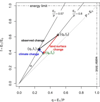
coor-dinate system. Such a water–energy partitioning diagram is shown in Fig. 1 with the two states corresponding to differ-ent climatic (i.e.,φ=E0/P) and hydrological conditions
ex-pressed asET. The line from origin whereET= 0 through a
respective point (q,f) corresponds to a fixed aridity index. Hence, we define a land-surface change by a change inET
0.0 0.2 0.4 0.6 0.8 1.0
0.0
0.2
0.4
0.6
0.8
1.0
q=ET P
f
=
ET E0
P= E0
●
● ● climate change
land surface change observed change
energy limit
w
ater limit
w
ater limit
E0
P=0.8
E0
P=0.57
α (q1,f1)
(q0,f0)
(qb,fb)
Fig. 1. Illustration of the separation of climate and land-surface
changes in a q–f space diagram. The example shows two
hy-droclimatic states before (q0, f0) and after transition (q1, f1).
The position of point (qb, fb) is determined by using the
de-scribed geometric approach. The bold arrow lines depict the cli-matic and the land-surface components of this transition. For
il-lustration we used case conditions of a base state:P0= 1000 mm,
E0,0= 800 mm,ET ,0= 500 mm and a state after hypothetical cli-matic and land-surface change withP1= 1400 mm,E0,1= 800 mm,
ET ,1= 350 mm. TherebyETdecreased by 30 %.
but constant aridity. In the water–energy partitioning plot, the land-surface change direction is determined by the inverse of the aridity indexP /E0. Next, we define climatic changes as
changes in the aridity index which correspond to a change to a differentφline. Note, that this step is a major simplifica-tion in defining impacts of climatic changes and land-surface changes onET. Hence climatic changes are very strictly
de-fined as changes in the average supply of water and energy. All other changes are referred to as land-surface changes, including direct human impacts such as land use and envi-ronmental pollution, as well as indirect effects due to green-house gas emissions and global warming. This also includes changes in the variability of climatic drivers.
Still, one problem remains, as we still need to define the direction of climatic changes within the water–energy dia-gram. Here we simply adopted the orthogonality assumption of Tomer and Schilling (2009) and assume that the climatic direction is perpendicular to the originalφrelated line. This implies that climatic impacts are independent of the catch-ment response (ET). Hence, at any point along a constant
aridity index (a line with the slope of P /E0) the climate
With the above assumptions we can derive the magnitude of both climate and land-surface related changes also for the case of simultaneous impacts. The derivation can be done in the cartesian space described byq=ET/P andf=ET/E0.
Furthermore, we consider two observed points in this space (q0,f0) and (q1,f1). The angle between both vectors can be
described by the scalar product divided by the vector magni-tudes to give
sin(α)= q0f1−q1f0
q
q02+f02 q
q12+f12
. (3)
Further the orthogonality assumption states that the cli-mate change direction is perpendicular to the aridity index line on (q0,f0). Hence we seek the coordinates of point (qb,
fb) which is an intermediate state consisting of the
land-surface change component and the climate change compo-nent of the observed changes. Again the sine ofαcan be re-lated to the line segment of ((q1, f1); (qb, fb)) and the
mag-nitude of point (q1,f1):
sin(α)=
q
(qb−q1)2+(fb−f1)2
q
q12+f12
. (4)
Combining both Eqs. (3) and (4) and substituting
fb=qbf0/q0yields thexcoordinates of point (qb,fb):
qb =
f0f1q0+q02q1
f02+q02 . (5)
As it is defined that a land-surface change alters evapotran-spiration at a constant aridity index,ET,bat point (qb,fb) can
then be computed fromqband the initial climatic conditions:
ET,b=qbP0.
The absolute differences of the observed evapotranspira-tion rates (ET,0, ET,1) to ET,b can then be used to
deter-mine the climatic (1ET,C) and land-surface (1ET,L) parts of
change:
1ET,L=ET,b −ET,0 (6)
1ET,C=ET,1−ET,b. (7)
Because this simple geometric approach is applied to discrete differences in a non-linear diagram, it remains somewhat ar-bitrary if we assume orthogonality at point (q0,f0) or point
(q1, f1). If the differences would be infinitesimally small
than it would make no difference at which point we assume orthogonality. So, ideally we might use an integral of these small changes. For the geometrical approach this would yield a circle equation with origin at (0, 0) and a radius defined by the point in the diagram. However, this step would compli-cate the approach and the differences are small compared to the overall changes and the detection thereof (changes inET,
P,E0).
The proposed method can in principle be applied to any reasonable hydro-climatic state, however, whenET is close
to a limitation (ET/P→1 orET/E0→1) then the
orthog-onality assumption violates the first principles of mass and energy conservation. Hence, accounting for water limita-tion or energy limitalimita-tion implies that the catchment response
ET must also be taken into account. Yang et al. (2008)
show that this yields the Mezentsev (1955) or Choudhury (1999) parametric Budyko function. The Choudhury equa-tion only yields an orthogonal response of climate to land-surface change, when its parameter is set ton=2 which is identical to the classic Pike (1964) equation. Other classic Budyko curves (Schreiber, 1904; Ol’Dekop, 1911; Budyko, 1948) are similar but yield not exactly orthogonal responses ofETto climate. Also note that the climate elasticity studies
of Dooge (1992) and Arora (2002) use the slope at a given aridity index of these classic Budyko functions. Hence, these studies derive the climatic sensitivity also independently of the actual catchment response. By employing a parametric Budyko curve such as the Choudhury (1999) or the Fu (1981) curve, the effect of the catchment response can be taken into account (Yang et al., 2008; Roderick and Farquhar, 2011). At higher n(or ET) the Choudhury curve is more bent
to-wards the limits, whereas atn <1 the curve bends towards (ET/P →0 or ET/E0→0). To our knowledge, however,
there exists no empirical evidence of these mathematically derived sensitivities ofET to changes in climate, whennis
smaller than 1.
Similar studies on separating climate from land-surface changes directly employ a Budyko type of function to predict the climate related change inETand attribute the difference
to a land-surface impact (Wang and Hejazi, 2011; Jaramillo et al., 2013). In contrast the presented geometrical separation method has the benefit that it does not require a Budyko type of function for application.
3 Study area and database
In the following a brief overview of the study areas is pro-vided, followed by a description of the data base.
3.1 Study area
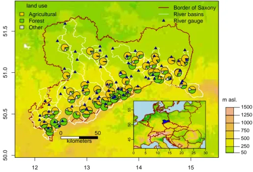
12 13 14 15
50.0
50.5
51.0
51.5
0 50
kilometers
Border of Saxony River basins River gauge land use
Agricultural Forest Other
50 250 500 750 1000 1250 1500 m asl.
0 5 10 15 20 25 30
45
50
55
Fig. 2. Topography of the Federal State of Saxony/Germany, river basin divides, river gauging stations and dominant land use. The blue polygon in the inset shows the border of Saxony within central Europe.
to the colder climate, mountainous topography and less fer-tile soils, these parts are mainly covered by forests, whereas the lower regions are agriculturally dominated. The ratio of forest to agricultural land use is reported on a catchment ba-sis in Fig. 2.
Land use and land cover in eastern Germany have been af-fected by changes in agricultural policies after World War II (Baessler and Klotz, 2006). Especially during the “collec-tivization” period (1952–1968) small farms were pooled to form large agricultural producers’ cooperatives (“LPG”). However, 1990 marked another major turning point in agri-cultural policy, with the privatization of agriagri-cultural land fol-lowing the political changes in the former East Germany (Eckart and Wollkopf, 1994). The proportion of agricultural land has decreased from 57 % in 1992 to presently 55 % of the area of Saxony (StaLa, 2012), of which around 23.7 % is used as pasture. Forests cover at present in total 27.2 % of the state’s area (in comparison to around 26 % in 1992). For-est vegetation was heavily impacted by air pollution, with subsequent tree die-off since the 1960s and with major clear cuts in the 1980s (Šrámek et al., 2008) at the mountain ridge in southern Saxony. Such dramatic changes in vegetation cover may have also influenced hydrologic processes. Be-tween 1991 and 2012, the proportion of damaged forest de-creased from 27 to 16 % of the total forested area (SMUL, 2006). Urban and infrastructure areas have increased from around 10 % in 1992 to 12.6 %.
3.2 Runoff data
The Federal State of Saxony operates a dense network of hy-drological gauging stations with a rich set of locations hav-ing long observation histories. The network density further increased in the 1960s. We have chosen river gauge stations, which almost fully cover the period 1960–2000. The daily discharge data have been converted to monthly runoff depth (mm month−1) using the respective catchment area. Then
runoff data were subjected to a homogenization test proce-dure; first on the runoff ratio (Q/P), and second using the weighted mean reference series of neighboring catchments. We also removed basins with large dams, compared to basin size. The remaining 68 stations cover large parts of Saxony, with catchment areas ranging from 5 to 6171 km2. Most sta-tions are within the Mulde River basin (23) or are located at the tributaries of the Upper Elbe (18). Note, that some of the stations are directly connected and are not independent. Detailed information can be found in Table S1 in the Supple-ment. The locations of the gauging stations and catchment areas can be found on the map provided in Fig. 2. All further procedures are based on annual values using the definition of hydrological years (1 November to 31 October).
3.3 Precipitation data
interpolation. To account for the height dependency, a lin-ear height relationship was established using a robust median based regression (Theil, 1950). Then the residuals have been interpolated onto an aggregated SRTM grid (Jarvis et al., 2008) of 1500 m raster size using an automatic ordinary krig-ing (OK) procedure (Hiemstra et al., 2009). Annual basin av-erage precipitation is then computed by the weighted avav-erage of the respective grid cells. The method of height regression and OK of the residuals was chosen, as this method showed to have the lowest root mean square errors (RMSE) among other methods, in a cross-validation based on annual station data sets (not shown).
Besides the spatial interpolation uncertainty, two other sources of uncertainty dominate the annual precipitation es-timates time series. First, there is a precipitation bias. To ac-count for this effect, we performed a precipitation correc-tion of the annual precipitacorrec-tion sums using the Richter (1995) scheme which is largely based on rain gauge sheltering fac-tors and altitude. The bias correction only led to a shift in pre-cipitation related data, but did not change the overall features. For further analysis, we used the uncorrected values. A sec-ond uncertainty is the varying number of available stations in the domain. To account for this problem, three different sets of interpolated precipitation time series have been produced, (a) fixed net of stations covering the full period and (b) all available stations at a time. We assessed the differences and opted for a compromise between (a) and (b) with stations covering large parts of the core period 1960–2000.
3.4 Potential evaporation
To describe the evaporative demand we employ a parametric potential evapotranspiration scheme. This has the advantage of the use of standard meteorological data for estimation. Donohue et al. (2010) have shown that trends in various input data can lead to different trends inE0 depending on which
scheme and thus input variables have been used. Thereby the physically based Penman scheme yielded the most reason-able magnitudes and trends (Donohue et al., 2010).
For annualE0estimates we make use of the FAO (Food
and Agricultural Organization) grass reference evapotranspi-ration method (Allen et al., 1994). This simplification of the Penman–Monteith equations is widely used as it provides many alternative ways to use available input data. Here we first compiled monthly averages of daily station data of tem-perature (mean, minimum, maximum), sun shine duration, relative humidity and wind speed data. The locations of the climate stations used are shown as dots in Fig. 3b. The ag-gregated annual totals were then spatially interpolated with an automatic universal kriging procedure with station eleva-tion as local trend variable (Hiemstra et al., 2009).
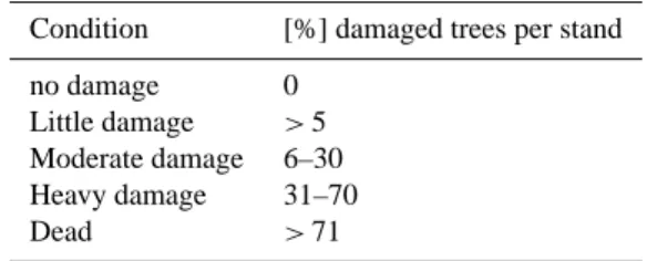
Table 1. Forest damage classification.
Condition [%]damaged trees per stand
no damage 0
Little damage >5
Moderate damage 6–30
Heavy damage 31–70
Dead >71
3.5 Land cover and vegetation data
The characterization and quantification of hydrological ef-fects of land-surface changes such as land use change or for-est damage would ideally require several temporal snapshots over the study area. Here, we use the satellite based Corine land cover data set and forest damage data to assess forest health over time.
3.5.1 Corine land cover classification
For the assessment of dominant land cover types in the an-alyzed catchments, we used the Corine Land Cover raster data set of the year 2000 available from the European En-vironment Agency (EEA). The data show different levels of land cover classes and aggregated types of forested and near natural vegetation classes are combined as “forest”, whereas all agriculturally and grass lands are merged as class “agricultural”.
To compute the area of damaged forest within a catch-ment, we used the Corine land cover class transitional scrub forest (324). This land cover class includes areas of dam-aged forests (cf. Bossard et al., 2000). A visual comparison showed good agreement of these maps with the forest dam-age maps in Fig. 7d.
3.5.2 Forest damage data
12.0 12.5 13.0 13.5 14.0 14.5 15.0 50.5 51.0 51.5 ● ● ● ● ● ● ● ● ● ● ● ● ● ● ● ● ● ● ● ● ● ● ● ● ● ● ● ● ● ● ● ● ● ● ● ● ● ● ● ● ● ● ● ● ● ● ● ● ● ● ● ● ● ● ● ● ● ● ● ● ● ● ● ● ● ● ● ● ● ● ● ● ● ● ● ● ● ● ● ● ● ● ● ● ● ● ● ● ● ● ● ● ● ● ● ● ● ● ● ● ● ● ● ● ● ● ● ● ● ● ● ● ● ● ● ● ● ● ● ● ● ● ● ● ● ● ● ● ● ● ● ● ● ● ● ● ● ● ● ● ● ● ● ● ● ● ● ● ● ● ● ● ● ● ● ● ● ● ● ● ● ● ● ● ● ● ● ● ● ● ● ● ● ● ● ● ● ● ● ● ● ● ● ● ● ● ● ● ● ● ● ● ● ● ● ● ● ● ● ● ● ● ● ● ● ● ● ● ● ● ● ● ● ● ● ● ● ● ● ● ● ● ● ● ● ● ● ● ● ● ● ● ● ● ● ● ● ● ● ● ● ● ● ● ● ● ● ● ● ● ● ● ● ● ● ● ● ● ● ● ● ● ● ● ● ● ● ● ● ● ● ● ● ● ● ● ● ● ● ● ● ● ● ● ● ● ● ● ● ● ● ● ● ● ● ● ● ● ● ● ● ● ● ● ● ● ● ● ● ● ● ● ● ● ● ● ● ● ● ● ● ● ● ● ● ● ● ● ● ● ● ● ● ● ● ● ● ● ● ● ● ● ● ● ● ● ● ● ● ● ● ● ● ● ● ● ● ● ● ● ● ● ● ● ● ● ● ● ● ● ● ● ● ● ● ● ● ● ● ● ● ● ● ● ● ● ● ● ● ● ● ● ● ● ● ● ● ● ● ● ● ● ● ● ● ● ● ● ● ● ● ● ● ● ● ● ● ● ● ● ● ● ● ● ● ● ● ● ● ● ● ● ● ● ● ● ● ● ● ● ● ● ● ● ● ● ● ● ● ● ● ● ● ● ● ● ● ● ● ● ● ● ●● ● ● ● ● ● ● ● ● ● ●
Average annual precipitation totals
200 400 600 800 1000 1200 1400 P [mm]
12.0 12.5 13.0 13.5 14.0 14.5 15.0
50.5 51.0 51.5 ● ● ● ● ● ● ● ● ● ● ● ● ● ● ● ● ● ● ● ● ● ● ● ● ● ● ● ● ● ● ● ● ● ● ● ● ● ● ● ● ● ● ● ● ● ● ● ● ● ● ● ● ● ● ● ● ● ● ● ● ● ● ● ● ● ● ● ●
Average annual potential evapotranspiration totals
600 650 700 750 800 850 900
E0 [mm]
12.0 12.5 13.0 13.5 14.0 14.5 15.0
50.5 51.0 51.5 ● ● ● ● ● ● ● ● ● ● ● ● ● ● ● ● ● ● ● ● ● ● ● ● ● ● ● ● ● ● ● ● ● ● ● ● ● ● ● ● ● ● ● ● ● ● ● ● ● ● ● ● ● ● ● ● ● ● ● ● ● ● ● ●● ● ● ●
Average annual runoff
0 200 400 600 800 Q [mm]
12.0 12.5 13.0 13.5 14.0 14.5 15.0
50.5 51.0 51.5 ● ● ● ● ● ● ● ● ● ● ● ● ● ● ● ● ● ● ● ● ● ● ● ● ● ● ● ● ● ● ● ● ● ● ● ● ● ● ● ● ● ● ● ● ● ● ● ● ● ● ● ● ● ● ● ● ● ● ● ● ● ● ● ●● ● ● ● 100 200 300 400 500 600
P−Q [mm]
Average annual water balance residual, ET = P − Q
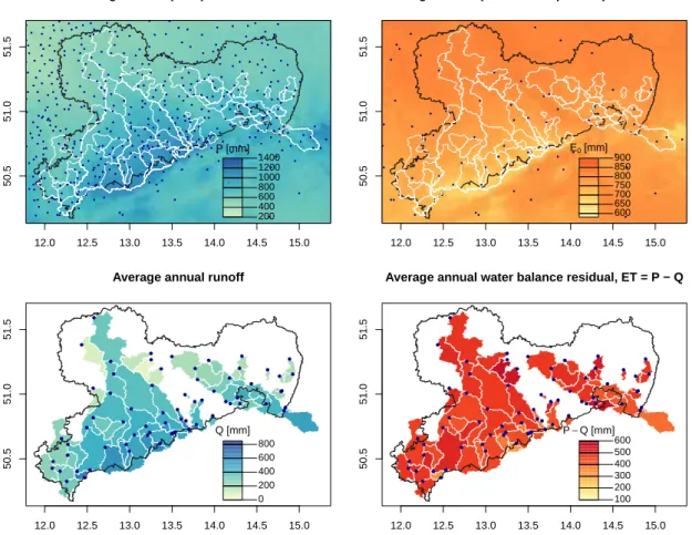
Fig. 3. Maps of long-term (1950–2009) annual average values for (a) precipitation, (b) annual potential evapotranspiration (FAO-Reference, Allen et al., 1994), (c) annual runoff and (d) the residual water budgets (ET=P−Q). Observation stations are depicted as dots. The maps
of annual average of precipitationP and the FAO reference potential evapotranspirationE0have been derived by averaging the individual
annual raster maps used to calculate the basin averages. Note, that each graph has its own color scale.
4 Results
4.1 Hydroclimatology of Saxony
In this section the long-term average (1950–2009) hydrocli-matology of Saxony is illustrated based on the established data set.
Annual average observed station precipitation within the study area ranges between 425 and 1340 mm yr−1 and has a distinct north to south increasing gradient which is linked to topography. Another, although weaker gradient is induced by the transition of maritime to continental climate which re-sults in decreased precipitation from west to east (Fig. 3a). The calculated FAO reference potential evapotranspiration
E0 ranges between 554 and 881 mm yr−1and is negatively
correlated with precipitation showing a decrease with higher elevation (see Fig. 3b). Runoff largely follows the precipita-tion gradients showing the lowest annual values in the north (minimum 63 mm yr−1) and increasing with height in the south (maximum 824 mm yr−1). As visible from Fig. 3c, the runoff pattern is dominated by the Mulde River basin which
receives a large share of its water from the headwater catch-ments in the Ore Mountains. By closing the water balance we estimate actual catchment evapotranspiration (Fig. 3d). The lowest values of annualETare found in the high headwater
basins (minimum 188 mm yr−1). The pattern of the higher
ET (>500 mm yr−1) is more complex. These patterns are
predominantly found in areas of large potential evapotran-spiration (north and east), but also in areas with high annual precipitation and relatively gentle slopes such as in the south-western part. All long-term average data can also be found in Table S1 (Supplement).
Table 2. Altitude effects on climate, water–energy balance, groundwater influence (estimated as one year lag cross-correlation coefficient of precipitation and runoff,ρPt−1;Qt) and percentage of forest cover. Reported are Pearson correlation coefficients for the long-term averages
of all basins. All relations are significant withp <0.001.
Altitude φ P E0 ET/P ET/E0 ρPt−1;Qt
Altitude
φ −0.93
P 0.93 −0.99
E0 −0.98 0.90 −0.89
ET/P −0.89 0.91 −0.91 0.86
ET/E0 −0.65 0.58 −0.61 0.61 0.86
ρPt−1;Qt −0.72 0.62 −0.67 0.68 0.70 0.65
Forest cover 0.78 −0.75 0.76 −0.78 −0.77 −0.62 −0.57
1950 1960 1970 1980 1990 2000 2010
400
600
800
1000
1200
1400
E0
,
P
[mm]
P, annual basin data P, decadal average E0, annual basin data
E0, decadal average
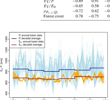
Fig. 4. Time series of annualP andE0 for all basins and the all
basin decadal averages.
Variability of annual precipitation and potential evapotranspiration
To get an overview of the temporal dynamics ofP andE0
we plot time series of both variables for all catchments in Fig. 4. For precipitation, a large temporal variability can be observed for all basins, but with considerable spatial coher-ence. Because of the large natural variability there are hardly any significant signals of structural changes in basin precip-itation. We only find a gentle decrease after 1960 and an in-crease since about the 1990s.
We estimated the evaporative demand by using the FAO reference potential evapotranspiration. This series shows less year to year variability and much stronger spatial coherence than precipitation (see Fig. 4). From the data, we observe a period of lower averageE0 between 1960 and 1990 with
a significant increase after 1990. This structural change is also found in observations of sunshine duration (not shown). With regard to the aridity index8=E0/P the observed trend
changes inE0are, however, much smaller than the variability
ofP and thus not detectable in a8series.
1940 1960 1980 2000
0
200
400
600
800
P − Q
% damaged forest area [0,0.01] (0.01,2] (2,20] (20,80]
Fig. 5. Time series ofP−Qin the period 1930–2009, where runoff
data was available. The thin lines show annual data of all catch-ments. In bold are 11 yr moving averages of certain groups of basins. The grouping and coloring follows the range of damaged forest area per basin using the Corine 1990 class 324 (transitional scrub forest). Note that for the 11 yr averages (bold lines) all avail-able data of each group have been used.
4.2 Variability of basin evapotranspiration
By taking the annual water budget residualP−Q, we an-alyze the interannual variability in basin scale ET,
how-ever, including the unknown influence of past water storage changes (1Sw). The annualP−Qdynamics are plotted in
Fig. 5. For the plot all basin data within the period 1930– 2009 are used. The interannual dynamics are consistent over the basins analyzed with significant influence of the interan-nual variability in aninteran-nual precipitation and potential evapo-transpiration. In the long run, the average water storage term can be assumed to diminish, hence we smooth the data us-ing a 11 yr movus-ing average in Fig. 5. To investigate if forest damage may have affected basin scaleET, we classified the
● ●● ●
● ●●
●
●
● ●
●
● ● ●
● ●
● ●
● ● ● ●
● ●
●● ● ●
● ●
● ● ●
● ●●
● ●
●● ●● ●
● ● ● ● ●
●●●●● ●
● ●
●
● ● ● ●●
● ●●
● ●
0.0 0.5 1.0 1.5
0.0
0.2
0.4
0.6
0.8
1.0
Φ =E0 P
(
P
−
Q
)
P
water limit
energy limit
Budyko curve land use
Agricultural Forest Other
●
●●
●
● ● ●
●
●
●
●
●
●
● ●
●
● ●
●
● ● ● ● ● ● ●● ●
●
● ●
●
● ● ● ●●
● ●
●● ● ●
●
●
●
● ●
●
● ●●●
● ●
●
● ●
●
● ●●●
● ●
● ● ●
0.2 0.4 0.6 0.8
0.2
0.4
0.6
0.8
q=ET P
f
=
ET E0
φ=
0.6
φ =0.8 φ = 1
φ =1.2 100
100
200 300
400
500
600
700
800
900
1000
Budyko curve
Fig. 6. Long-term (1950–2009) basin climate and water balance plots showing the Budyko space plot in the left and the water–energy partitioning plot in the right panel. The pie-charts show the areal percentage of land use of each basin. In the right panel, the average basin elevation is used to predict the contour lines using LOESS regression. This demonstrates the general height dependency of the basins climate. Further, the transition from wet basins with high runoff ratio to lower values is also reflected by land use.
snapshot without detailed knowledge of the magnitude and start of the forest damage it clearly indicates an area which has been significantly changed in the past. Using this clas-sification we found that 38 % of the basins have no dam-age (<0.01 %), 21 % have minor affected areas (0.01–2 %), 31 % have considerable damaged areas (2–20 %), and 10 % of the basins have damaged areas larger than 20 %. We used this classification to compute the group moving averages of
P−Q. For the first period from 1930 to about 1960, no large deviations between these groups can be observed although larger decadal scale variability was evident. After 1960 the series start to deviate strongly with the damaged areas show-ing a significant decline inP −Q. Since the 1980s the trend has reversed and there is a general increase in all groups. However, the group with the highest proportion of damaged forest shows the strongest increases towards the 1990s and 2000, with smaller deviations between these groups. The damaged group of basins show similar high values to those observed in the 1950s, whereas the other basins show even higherP−Qvalues. Already from Fig. 5 it can be deduced that forest damage can explain the larger deviations in basin scale evapotranspiration. Further, climatic variability which is rather coherent over the area of Saxony, shows a distinct effect, although of smaller magnitude.
4.3 Separation of climate and land-surface impacts on
ET
Having detected the influence of both, land-surface and cli-matic changes on basin scaleET, we now employ the
sepa-ration method illustrated in Sect. 2 to attribute the observed variability ofET to the variability in the aridity of climate
and the land-surface variability. We first illustrate the separa-tion framework in a cross-basin analysis of long-term annual average conditions and then apply the separation using the water–energy partitioning diagrams on the decadal timescale. Finally, we test the attribution approach by using the inde-pendent forest damage data.
4.3.1 Cross-basin analysis of climate and land-surface
impacts
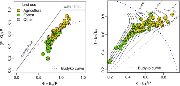
To illustrate the influence of the climate on long-term average evapotranspiration we use the classical Budyko curve which is shown in Fig. 6. The evaporation ratio ((P−Q)/P) of the various catchments increases with increasing aridity index (8=E0/P), but there is considerable deviation from the
the-oretical Budyko curve. The reasons for that could be a bias inE0 andP basin estimates. However, such a bias would
shift the whole group of basins to the left or right, without changing the apparent slope. By adding land use information (derived from Corine and aggregated to forest and agricul-tural land cover ratios per basin), it seems that the dominant land use caused the deviation from the Budyko curve. Thus, basins with dominant agricultural land use are well above and a set of forested basin are found well below the Budyko curve. However, a large part of basins, mainly with mixed type of vegetation, is still well represented by the Budyko curve.
Impacts of climate and land-surface conditions can be bet-ter represented by a wabet-ter–energy partitioning plot intro-duced with Fig. 1 which is populated with the same data as in Fig. 6. In Fig. 6, values in the lower left corner indicate low
corner most of the water and the energy is used for evapotran-spiration. To recap, the direction of change along an aridity line reveals dominant land-surface change impacts, whereas if the direction of change is perpendicular to an aridity line, the climatic change impacts are dominant. Besides land use information, we also depict the altitude dependency as con-tour lines within the water–energy partitioning plot. Note, that these contour lines follow approximately lines of con-stant aridity (dotted lines). That means the higher the altitude the more humid the climatic conditions. From the cross-basin correlation analysis we found that basin altitude and the arid-ity index are strongly, but negatively correlated (R=−0.93). Although some of the variability in water–energy partition-ing is explained by the aridity of the climate, many values in Fig. 6 stretch along these lines of constant aridity. This indicates that the largest variability within the set of basins is due to the variability of water–energy partitioning, rather than climate forcing. This variability is linked to land cover, as indicated by the pie charts. Hence, basins with a higher proportion of forests are located in the lower left corner, whereas the agricultural dominated basins largely are found in the upper right corner of the water–energy partitioning plot. These patterns thus support our assumption of differ-ent climate and land-surface change directions which were elaborated in Sect. 2.
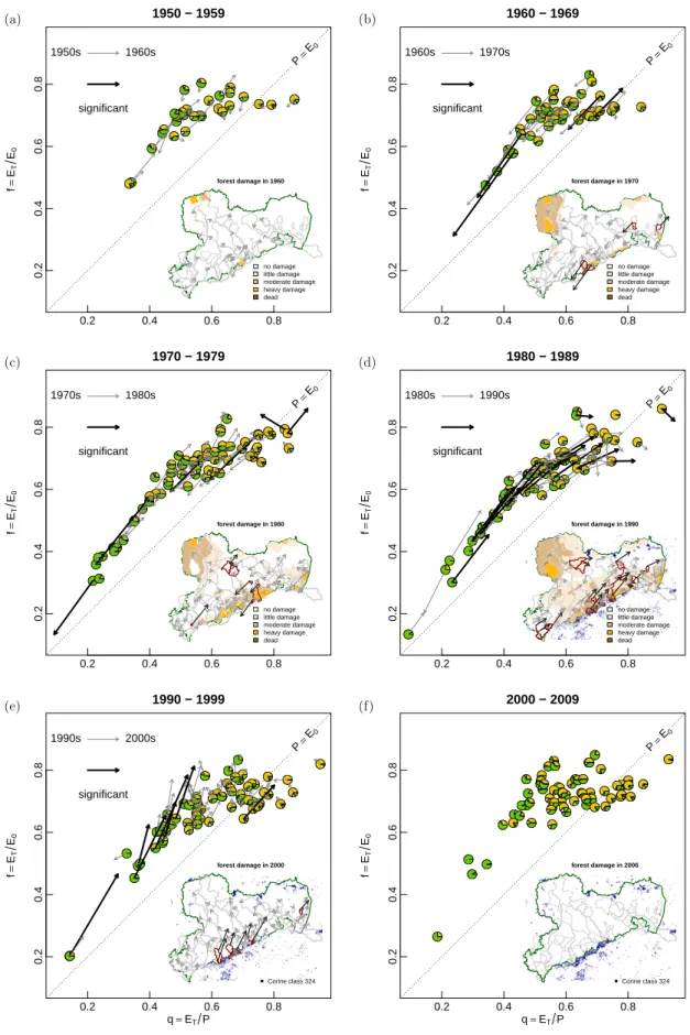
4.3.2 Decadal dynamics of water–energy partitioning
With Fig. 1 we illustrate that the direction of observed changes in the long-term average water–energy partitioning reveals the dominant impacts on hydroclimatology. We make use of this simple detection approach and plot the decadal averages in the water–energy partition diagrams in Fig. 7, where we assume that1Sw is negligible. We visualize the
change direction from one decade to the next with an arrow pointing to the average value of the next decade. Although the resulting trajectories are mostly coherent, we use a two sample Hotellings T2 test (Todorov and Filzmoser, 2009) with a significance level of α= 0.1 to denote any changes larger than the interannual variability caused by water stor-age changes. In the lower right of each panel a map of for-est damage in Saxony is drawn. Additionally, we show the trajectories using the river gauge location as origin of the re-spective arrow. This then helps to determine the locations and directions of dominant hydro-climatic changes and their re-lation to forest damage inventory data.
Looking at the decade 1950–1959 in Fig. 7a, we find the hydro-climatic conditions of the basins to be generally close, although not all basins were gaged at that time. The tra-jectories towards the 1960s are rather short and do not re-veal statistically significant changes. Some forest damages are located in smaller areas in the Ore Mountains along the southern border of Saxony and in the Leipzig lowlands in the northwest. Note, that the northwest and the northeast of Saxony have been highly impacted by open pit mining for
lignite (Grünewald, 2001). Due to massive hydraulic engi-neering, many river gauge records are very difficult to in-terpret in terms of evaporation changes and thus have been excluded from this analysis. Forest damages continued in-creasing during the 1970s and the trajectories showing the transition from the 1960s to the 1970s reveal a dominant land-surface change pattern with some significant changes mainly in the Ore Mountains and Upper Lusatia in the east (Fig. 7b). This pattern continues when we look at Fig. 7c with even more forests damaged and to a greater extent. Figure 7d shows a consistent and large upward trend in land-surface relatedET change along the Ore Mountains with the most
significant changes for the whole period. This land-surface related impact is accompanied with a change in the climatic forcing, namely the increase inE0(see Fig. 4), which is more
apparent in basins with higher water–energy partitioning ra-tios. In this case the higher atmospheric demand for water led to an increase of the water partitioning ratio (see Fig. 7d). At that time, reported forest damage was a major environmental issue affecting most of the forests in Saxony. Since 1990 also high-resolution remote sensing land cover classification can be used to identify forest damage on a transnational scale, which we show as blue raster cells at a 100 m spatial resolu-tion in the inset map. This shows hot spots of forest damages in the Ore Mountains, the Jizera Mountains and the North Bohemian Basin, also impacted by lignite mining and re-lated emissions. The water–energy plot in Fig. 7e shows con-tinuous increases inETwith dominant land-surface impacts
which are accompanied by a significant increase in precipita-tion (Fig. 4) when considering the changes from the 1990s to the first decade in 2000. In that case, increasing precipitation values with almost constantE0lead mainly to an increase of
the energy partitioning ratio, indicating a contribution of cli-mate variability. The comparison of the first decade (Fig. 7a) with the last decade (Fig. 7f) of the analysis reveals similar hydro-climatic states. This highlights a hydrological recov-ery of most of the forested basins and a dominance of the climatic aridity in controlling the variability ofET in these
decades.
4.3.3 Quantification of impacts
Using the geometric separation approach illustrated in Sect. 2.2, we computed the land-surface and climate related contribution of the observedETanomalies. As reference
pe-riod for computing the anomalies we choose the 2000–2009 decade, because of data availability and the side effect of having the highest ET values of the study period (Fig. 5).
● ● ● ● ● ● ● ● ● ● ● ● ● ● ● ● ● ● ● ● ● ● ● ● ● ● ● ● ●
1950 − 1959
0.2 0.4 0.6 0.8
0.2 0.4 0.6 0.8 f = ET E0 P= E0 1950s 1960s significant (a) no damage little damage moderate damage heavy damage dead
forest damage in 1960
● ● ●● ● ● ● ● ● ● ● ● ● ● ● ● ● ● ● ● ● ● ● ● ● ● ● ● ● ● ● ● ● ●● ● ● ● ● ● ●● ● ● ● 1960 − 1969
0.2 0.4 0.6 0.8
0.2 0.4 0.6 0.8 f = ET E0 P= E0 1960s 1970s significant (b) no damage little damage moderate damage heavy damage dead
forest damage in 1970
● ● ● ● ● ● ●● ● ● ● ● ● ● ● ● ● ●● ● ● ● ● ● ● ● ● ● ● ●● ● ● ● ● ● ● ● ● ● ● ● ● ● ● ● ● ● ● ● ●● ● ● ● ● ● ● ● ● ● ● ● ● ● ● ● ● 1970 − 1979
0.2 0.4 0.6 0.8
0.2 0.4 0.6 0.8 f = ET E0 P= E0 1970s 1980s significant (c) no damage little damage moderate damage heavy damage dead
forest damage in 1980
● ● ● ● ● ● ● ● ● ● ● ● ● ● ● ● ● ● ● ● ● ● ● ● ● ●● ● ● ● ● ● ● ● ● ● ● ● ● ●● ● ● ● ● ● ● ● ● ● ●● ●● ● ● ● ● ● ● ● ● ● ● ● ● ● ● 1980 − 1989
0.2 0.4 0.6 0.8
0.2 0.4 0.6 0.8 f = ET E0 P= E0 1980s 1990s significant (d) no damage little damage moderate damage heavy damage dead
forest damage in 1990
● ● ● ● ● ● ● ● ● ● ● ● ● ● ● ● ● ● ● ● ● ● ● ● ● ●● ● ● ● ● ● ● ● ● ● ● ● ●● ● ●● ● ● ● ● ● ● ● ● ● ● ● ● ● ● ● ● ● ●● ● ● ● ● ● 1990 − 1999
0.2 0.4 0.6 0.8
0.2
0.4
0.6
0.8
q=ETP
f = ET E0 P= E0 1990s 2000s significant (e)
Corine class 324
forest damage in 2000
● ●● ● ●● ● ● ● ● ● ● ● ● ● ● ● ● ● ● ● ● ● ● ● ● ● ● ● ● ● ● ● ● ● ● ● ● ● ● ● ● ● ● ● ● ● ●●● ● ● ● ● ● ● ● ● ● ●● ● ● ● ● ●
2000 − 2009
0.2 0.4 0.6 0.8
0.2
0.4
0.6
0.8
q=ETP
f = ET E0 P= E0 (f)
Corine class 324
forest damage in 2006
observed in the 1970s. In most basins the land-surface re-lated anomalies have the same sign as the climatic changes and show increasing dominance at higher altitudes, which is linked to the forest damages.
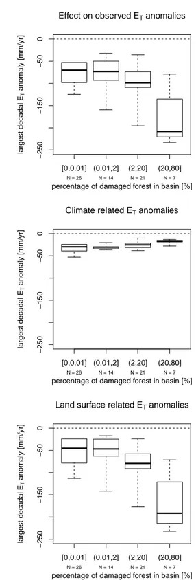
Combining hydro-climatic separation results with the for-est damage data allows for validation of the separation method. To do so we use the grouping of basins according to the damaged forest area per basin introduced with Fig. 5 to check if the forest damage has an effect on the attributed anomalies. Clearly for the land-surface related anomalies, we would expect that the larger the damaged area, the larger the
ETanomaly. In contrast, the climatic change impacts should
be independent of the land-surface impacts. The results of this test are shown in Fig. 8. The panels show the largestET
anomaly per basin grouped by the percentage of the dam-aged area. The climatic relatedET anomalies show a
gen-tle decrease in the magnitude of the anomaly with increas-ing forest damage. This effect is however much smaller than the increase of the absolute land-surface related anomalies with forest damage. There is hardly any distinction between basins without detected damages and damaged areas smaller than 2 %. Moderately affected basins between 2 and 20 % damage show a trend, whereas strongly affected basins show distinctly largerETanomalies.
5 Discussion
5.1 Controls on water–energy partitioning
The long-term average partitioning of water and energy in Saxony shows two dominant patterns. First, there is the con-trol by climatic conditions which is best described by the aridity index. This pattern reveals that under more humid conditions the energy limitation results in higher energy par-titioning ratios than water parpar-titioning ratios. Towards non-limited conditions (i.e.,P=E0) both ratios are also equal. In
Saxony, the humidity gradients are mainly driven by topog-raphy. We find that the orographically driven precipitation induces a gradient in available water and available energy forET. In general, the effects of the gradients inP andE0
should be predictable with a Budyko type of function. However, there is a second emergent pattern, which re-veals a large variability of water–energy partitioning along a fixed climate aridity index (Fig. 6). Hence both, energy and water partitioning ratios are simultaneously affected. We hy-pothesize that this pattern is linked to land-surface related conditions, which effectET, but also correlate with altitude.
A persistent control is the water storage capacity which is also linked to topography and the presence of aquifers (we used the lagged cross correlation of annual precipitation and runoff as proxy). This control shows a positive correlation toET(Table 2) as it determines the availability of water
un-der dry conditions. This finding is in line with Troch et al. (2013) who relate deviations from the Budyko curve to the
[0,0.01] (0.01,2] (2,20] (20,80]
−250
−150
−50
0
percentage of damaged forest in basin [%]
largest decadal
ET
anomaly [mm/yr]
Effect on observed ET anomalies
N = 26 N = 14 N = 21 N = 7
[0,0.01] (0.01,2] (2,20] (20,80]
−250
−150
−50
0
percentage of damaged forest in basin [%]
largest decadal
ET
anomaly [mm/yr]
Climate related ET anomalies
N = 26 N = 14 N = 21 N = 7
[0,0.01] (0.01,2] (2,20] (20,80]
−250
−150
−50
0
percentage of damaged forest in basin [%]
largest decadal
ET
anomaly [mm/yr]
Land surface related ET anomalies
N = 26 N = 14 N = 21 N = 7
Fig. 8. Largest decadalP−Q anomalies with respect to the last
timescale of a perched aquifer. Another land-surface con-trol is vegetation, which we assessed by land cover classi-fication, just separating into agricultural and forested basins. The type of land-use is naturally correlated to climate and water–energy partitioning, resulting in a negative correlation with forest cover, which is again well correlated with alti-tude and thus climate aridity. The rather high correlations of land-surface properties to climate reveals strong interac-tions between climate, soils and vegetation. This equilibrium state may explain the predictive power of the Budyko curve (Gentine et al., 2012).
An intriguing finding of our study, however, is that even on the long term two sets of basins substantially deviate from the Budyko curve. These are low altitude agriculturally dominated basins which are well above the Budyko curve, whereas a set of forest dominated basins exhibit rather small
ET/P and ET/E0 ratios. A few agricultural basins show
larger decadal dynamics in water–energy partitioning, espe-cially in the 1960s to 1990s. Although some change may be attributed to land management changes towards industrial-ization of agriculture (Eckart and Wollkopf, 1994; Baessler and Klotz, 2006), the patterns, however, are not very consis-tent and no detailed data on land management changes was available for this study to identify potential causes. In this study, we focussed on the causes of the low water–energy partitioning ratios of some of the forested basins. The forest damage data revealed that the decadal changes in the water– energy partitioning are due to the forest decline, which ex-plains why these basins are well below the Budyko curve. In the following, we discuss the role of non-stationary changes detected in the water–energy partitioning of these basins.
5.2 The role of environmental pollution on regional
scaleET
Although we discussed the impacts of climate and land-surface change separately, there is some evidence that both have been caused by heavy air pollution throughout central Europe. The aerosol emissions of the coal power stations have led to decreases in surface solar radiation also known as the “global dimming” (Wild et al., 2005), peaking in the 1980s (Ruckstuhl et al., 2008; Philipona et al., 2009). This has had a direct effect on the evaporative demand, which caused a significant reduction in potential evapotranspiration during that time (Fig. 4).
The indirect effects of the air pollution have been more localized due to topographical and meteorological factors fa-voring an inversion (Pfanz et al., 1994). An inversion typi-cally leads to frequent foggy conditions, particularly in the mountain ridges (Flemming, 1964). Due to the air pollution the aerosol load in the fog reached very high concentrations (Schulze, 1989; Zimmermann and Zimmermann, 2002). The deposition of the aerosols led to an accumulation of sul-furous acid and other pollutants in the soils (Pfanz et al., 1994; Zimmermann et al., 2003). This effect was especially
dominant in coniferous forests, which tend to comb out fog due to their large capacity for water interception (Lange et al., 2003). Over time the acidified soils led to changes in the nutrient compositions with reduced magnesium and calcium cations in the soil solution (Schulze, 1989). This resulted in severe tree crown damages, reduced stand pro-ductivities and higher vulnerability for other environmental stress factors (Sterba, 1996; Wimmer et al., 2002). Evapo-ration from interception as well as transpiEvapo-ration must have been drastically reduced by the affected trees, thus affecting both of the processes dominant in shaping total evaporation. The importance for basin scale evapotranspiration is evident from Fig. 5, as well as the decadal water–energy partition-ing plots in Fig. 7. The decadal changes highlighted in Fig. 7 show that many higher altitude, forested basins moved along relatively constant aridity lines. These changes are attributed to land-surface change, but the timing of these changes is not synchronized across all catchments. A possible explanation is that the timing of the dominant hydrological effects of the forest damage can differ strongly due to the actual damage and forest management actions such as clear cutting of dam-aged stands.
The phenomena of the Waldsterben appeared on the polit-ical agenda in the 1980s and resulted in a common call for reducing power plant emissions. Additionally, the transition from the 1980s to the 1990s marks a period of drastic po-litical, socio-economic changes in the former East Germany and eastern Europe. The industrial breakdown especially ac-celerated the improvement of environmental conditions and significantly reduced aerosol emissions (Matschullat et al., 2000; Zimmermann et al., 2003). The reduced aerosol emis-sions quickly increased surface solar radiation, temperatures (Philipona et al., 2009) and, as evident from Fig. 5, alsoET
across all basins reaching among the largest values of the study period.
Interestingly, the catchments with damaged forests also show stronger increases in ET (Fig. 5) consistent over all
catchments along the Ore Mountains (see Fig. 7d). This quick and consistent recovery ofET highlights the
impor-tance of understorey and young stands taking over key roles of water and energy partitioning. This fast recovery of ET
might also explain the sign differences of significant water– energy trajectories before 1990 and thus the difficulty in assessing the timing of hydrological impacts of vegetation changes. Together with relatively poor observations describ-ing relevant hydrological land-surface characteristics, this difficulty reduces the predictive power for single basin ET
dynamics from forest damage data alone.
5.3 Potentials and limitations
may occur simultaneously, but act on different processes and thus scales, including internal responses to these external forcings. The proposed framework, based on mass and en-ergy conservation, may be regarded as the simplest possible first order approach. The separation requires a few strong as-sumptions, which makes this a transparent and attractive ap-proach for research and practitioners.
The method can be used to identify non-stationary changes in the average water–energy partitioning and to quantify the contributions of the most general impacts (Renner and Bernhofer, 2012). It is, however, important to note that due to the strict definition of climatic change impacts, and the more open definition of land-surface change impacts it is not possible to directly trace the respective process causing the observed change. To identify the role of sub-scale processes, process-based models are required. As these models gener-ally require more input data, they additiongener-ally suffer from model parameter and model structure uncertainties (Seibert and McDonnell, 2010). Hence, these more detailed analyses should be approached in a top-down manner (Klemeš, 1983), starting with a simple first order approach as illustrated here. The proposed method is prone to input data uncertain-ties, especially precipitation, potential evapotranspiration and runoff data. However, if we assume that random errors average out over longer periods as used here, these uncertain-ties may diminish. We also tested the influence of systematic uncertainties, such as precipitation bias correction, station network changes, the estimation of potential evapotranspi-ration, or the uncertainty of deriving spatial basin scale me-teorological input data. All of these play a role but resulted in shifting the whole data set rather than changing its shape within the water–energy partitioning plots.
In this analysis, the uncertainty of land-surface related changes was dominant. This is most apparent in Fig. 8c where we analyze the effect of forest cover damage on the land-surface relatedETanomalies. First, there is a large
vari-ability across basins, but also note that the land-surface re-lated anomalies are significantly below zero also in basins where no forest-damage has been detected. Apparently, the land-surface related anomalies are on the order of the cli-mate related impacts, which may highlight the uncertainty range of the approach. Yet, it is not clear if the dominant uncertainty arises from the separation method, other land-surface related changes, the input data, or changes in water storage at the chosen averaging periods. However, we argue that the consistence of negative land-surface related anoma-lies over the study area may rule out the latter two. Appar-ently, there is a background signal of increasing ET in all
catchments which is attributed to land-surface changes. Sim-ilar increases inET have been found in the US by Walter
et al. (2004) and Renner and Bernhofer (2012). This could indeed be land cover induced changes, for example increas-ing vegetation growth (McMahon et al., 2010), or increasincreas-ing human water use for food and energy production (Destouni et al., 2013). But also changes in meteorological variables
not covered in the long-term annual average aridity index may have induced this signal. Hence, the identification of the causes of the recent land-surface attributed increases inET
should be addressed in further research.
Despite these limitations and the simplicity of the ap-proach, we have been able to show that the timing and spatial extent of forest damage can be linked to distinct land-surface related changes of basin scale ET. Whereas the anomalies
attributed to changes in climate aridity are almost indepen-dent from the magnitude of forest damage. This validates the usefulness of the separation framework for the assessment of hydro-climatic changes on decadal timescales.
6 Conclusions
Plotting the ratio of energy partitioningET/E0vs. the water
partitioning ratioET/P is a very useful tool to analyze
an-nual average evapotranspiration. This diagram allows for the investigation of the interplay of the water and energy balance and the tight coupling of both throughET. The diagram can
also help to differentiate between climatic and land-surface controls on ET. Both controls result in qualitatively
differ-ent patterns of water–energy partitioning. In particular, cli-matic changes, defined as changes in the aridity index, result in a shift in the diagram which is perpendicular to changes resulting from land-surface changes. This allows a geometri-cal separation and quantification of climatic and land-surface impacts onET.
Testing this approach with data of the well-observed re-gion of Saxony reveals some general insights on how and why this simple approach is successful. First, it is known that vegetation is adapting to climatic conditions and thus re-duces the influence of other land-surface conditions such as soils and topography on water–energy partitioning. Hence, long-term annual average ET can indeed be predicted by
the Budyko curve which only requires data on precipita-tion and evaporative demand. Second, the prevailing climate also determines the hydrological sensitivity to climatic or land-surface changes. Plotting the Budyko curve or decadal average data in water–energy diagrams reveals that adap-tion to changes in P or E0 result in opposing effects on
water and energy partitioning. A trend towards a more hu-mid climate will thus reduce the water partitioning ratio (ET/P), while the energy partitioning ratio (ET/E0) will
impacts such as environmental pollution adversely affecting vegetation functioning will lead to declines in ET (here
in the order of 200 mm yr−1 or 38 %) and thus produce
more runoff. The long-term observations also reveal that
ET can recover within the order of decades, although
eco-physiological states are far from being recovered yet. This approach can identify general drivers of change in landscape hydrology solely by using long-term observations of catchment runoff, precipitation and potential evapotran-spiration. Since the method is general, it can be transferred to other regions and other climate conditions. The relatively low data demand allows first order impact assessment of past climate and land surfaces as well as estimates on future cli-mate impacts on hydrology, without the need of numerical modeling.
Finally, we have to note that the simplicity of the approach does not allow to attribute certain changes to a more spe-cific process or cause. An intriguing example is that we found thatETconsistently increased in the last two decades (1990–
2009). According to the methods definitions, this increase is attributed to a land-surface change. Hence, all basins moved closer to the water and energy limits of evapotranspiration. Although this effect is smaller than the land-surface changes induced by the forest decline, it is of similar magnitude than increases inET caused by changes in P or E0. While this
points to the limits of the proposed approach, it also high-lights the potential role of other climatic variables to explain this increase in catchment scaleET. This should be addressed
in future research.
Supplementary material related to this article is
available online at http://www.hydrol-earth-syst-sci.net/ 18/389/2014/hess-18-389-2014-supplement.pdf.
Acknowledgement. We acknowledge the Saxon State Office for the
Environment, Agriculture and Geology (LfULG) for providing the runoff time series and the German Weather Service (DWD), Czech Hydro-meteorological Service (CHMI) for providing climate data. M. Renner was kindly supported by Helmholtz Impulse and Networking Fund through Helmholtz Interdisciplinary Graduate School for Environmental Research (HIGRADE) (Bissinger and Kolditz, 2008). K. Brust acknowledges support from the German Research Foundation (DFG) grant BE 1721/13. We thank Bethany Shumaker and Lee Miller for checking and improving the language. The valuable comments of three reviewers are gratefully acknowledged.
The service charges for this open access publication have been covered by the Max Planck Society.
Edited by: S. Archfield
References
Allen, R., Smith, M., Pereira, L., and Perrier, A.: An update for the calculation of reference evapotranspiration, ICID Bull., 43, 35– 92, 1994.
Arnell, N.: Hydrology and Global Environmental Change, Pearson Education, Harlow, 2002.
Arora, V.: The use of the aridity index to assess climate change ef-fect on annual runoff, J. Hydrol., 265, 164–177, 2002.
Baessler, C. and Klotz, S.: Effects of changes in agricultural land-use on landscape structure and arable weed vegetation over the last 50 years, Agriculture, Ecosyst. Environ., 115, 43–50, doi:10.1016/j.agee.2005.12.007, 2006.
Bernhofer, C., Goldberg, V., Franke, J., Häntzschel, J., Harmansa, S., Pluntke, T., Geidel, K., Surke, M., Prasse, H., Freydank, E., Hänsel, S., Mellentin, U., and Küchler, W.: Klimamonographie für Sachsen (KLIMOSA) – Untersuchung und Visualisierung der Raum- und Zeitstruktur diagnostischer Zeitreihen der Kli-maelemente unter besonderer Berücksichtigung der Witterung-sextreme und der Wetterlagen, Sachsen im Klimawandel, Eine Analyse, Sächsisches Staats-Ministerium für Umwelt und Land-wirtschaft (Hrsg.), Dresden, p. 211, 2008.
Bissinger, V. and Kolditz, O.: Helmholtz Interdisciplinary Graduate School for Environmental Research (HIGRADE), GAIA – Ecol. Perspect. Sci. Soc., 17, 71–73, 2008.
Blöschl, G. and Montanari, A.: Climate change impacts’ throwing the dice?, Hydrol. Process., 24, 374–381, doi:10.1002/hyp.7574, 2010.
Bossard, M., Feranec, J., and Otahel, J.: CORINE land cover tech-nical guide: Addendum 2000, European Environment Agency Copenhagen, Copenhagen, Denmark, 2000.
Budyko, M.: Evaporation under natural conditions, Gidrometeoriz-dat, Leningrad, English translation by IPST, Jerusalem, 1948. Budyko, M.: Climate and life, Academic press, New York, USA,
1974.
Choudhury, B.: Evaluation of an empirical equation for annual evaporation using field observations and results from a biophys-ical model, J. Hydrol., 216, 99–110, 1999.
Dale, V. H.: The relationship between land-use change and climate change, Ecological applications, 7, 753–769, 1997.
Destouni, G., Jaramillo, F., and Prieto, C.: Hydroclimatic shifts driven by human water use for food and energy production, Nat. Clim. Change, 3, 213–217, doi:10.1038/nclimate1719, 2013. Donohue, R. J., Roderick, M. L., and McVicar, T. R.: On the
impor-tance of including vegetation dynamics in Budyko’s hydrological model, Hydrol. Earth Syst. Sci., 11, 983–995, doi:10.5194/hess-11-983-2007, 2007.
Donohue, R. J., McVicar, T. R., and Roderick, M. L.: Assessing the ability of potential evaporation formulations to capture the dy-namics in evaporative demand within a changing climate, J. Hy-drol., 386, 186–197, doi:10.1016/j.jhydrol.2010.03.020, 2010. Dooge, J.: Sensitivity of runoff to climate change: A Hortonian
ap-proach, B. Am. Meteorol. Soc. USA, 73, 2013–2024, 1992. Eckart, K. and Wollkopf, H.-F.: Landwirtschaft in Deutschland:
Veränderungen der regionalen Agrarstruktur in Deutsch-land zwischen 1960 und 1992, Institut für L anderkunde,
http://www.opengrey.eu/item/display/10068/216447 (last