PUBLICAÇÃO DA ABCM • ASSOCIAÇÃO
BRASILEI~A
DE CIÊNCIAS MECÂNICAS
REVISTA
BRASilEIRA DE CIÊNCIAS
MECÂNICAS
JOURNAL OF TiiE BRAZillAN SOCIE1Y OF MECJMNICAL SCIENCES
EDITOR:
leontrdo Goldstein Jr. UNICAMP- FEM- DETF - CP 6122 13083-970 Campinas. SP
Tel: (0192) 39-3006 fax: (0192) 39-3722 EDITORES ASSOCIADOS:
Agenor de Toledo Fleury
IPT - Instituto de Pesquisas Tecnológicas
Divisão de MecAnica e Eletrlcidade · Agrupamento de Sistemas de Controle Cidade Universitária- C.P. 7141
01064·970 São Paulo· SP
Tel: (011) 268-2211 R-504 faJ<: (011) 861)-3353 Carlos Alberto Carruco Altemani
UNICAMP- FEM- DE- C.P. 6122 13083·970 Campinas-SP
Tel: (0192) 39-8435 falC: (0192) 39-3722 José Augusto Ramos do Ama tal NUCLEN • NUCLEBRÁS ENGENHARIA. SA
Superintendência de Estruturas e Componentes Mecênicos. R: Visconde de Ouro Preto, 5
22250·180 · Rio de Janeiro- AJ
Tel: (021) 552-2772 R-269 ou 552·1095 Fax: (021) 552·2993 Walter L. Weingaertner
Universidade Federal de Santa Catarina Dep~ de Eno' Mecânica- lab. Mecânica de Precisão Campus • Trindade · C.P. 4 76
88049 Florianópolis -
se
Tel: {0482) 31·9395134-5277 Fax: (0482) 34·1519 CORPO EDITORIAL:
Alcir de Faro Orlando (PUC - RJ) Antonio Francisco Fortes (UnB) Armando Albertazzi Jr. (UFSC) Ata ir Aios Neto (INPE)
Benedito Moraes Purquerlo (EESC • USP) Caio Marío Costa (EMBRACO) Carlos Alberto de Almeida (PUC · AJ) Carlos Alberto Martin (UFSC) Clovis Raimundo Maliska (UfSC) Emanuel· Rocha Woiski {UNESP- FEIS) Francisco Emffio Baccaro Nigro (I PT • SP) Francisco José Simões (UFPb) Genesio José Menon (EFEI) Hans lngo Weber (UNICAMP) Henrique Rozenfeld (EESC USP) Jair Carlos Dutm (UFSC) João Atziro Hen de Jornada (UFAGS) José João de Espindola (UFSC) Jurandir ltizo Yanagihara (EP USP) Li rio Schaeter (UFAGS) Lourival Boehs (UFSC) Luís Carlos Sandoval Goes (ITA) Mareio Ziviani (UFMG) Moyses Zindeluk (COPPE • UFRJ) Nisio de Carvalho lobo Brum (COPPE • UFRJ) Nivaldo lernos Cupini (UNICAMP) Paulo Afonso de Oliveira Soviero (!TA) Paulo EiQi Mlyagl (EP USP)
Rogerio Martins Saldanha da Gama (lNCC) Valder Stetten Jr. (UFU)
REVISTA FINANCIADA COM RECURSOS 00
Programa de Apoio
a
Publicações CientificasMCT
~
CNPq
[2)
FINEP
RBCM • J. of thl Braz. Soe. Mechanlcal Sclencea Vol. XVII- n•4 • 1Q95 • pp. 344-352
ISSN 0100-7388 Printed in Brazll
A Computational Strategy for Determining
Bifurcation Diagrams for Non-Linear
Oscillating Systems
Paulo Batleta Gonçalves
Pontiftcie UniVersidade Catól1ca do Rlo de Janeiro Departamento de Engenharia CMI
22463-900 Rio de Janeiro. RJ Brasil
Vera Lúcia Slnjeb da S. Machado
UnlYeraidade Fedenal do Rio de Janeiro
Departamento de Mecênk:a Aplicada e Estruturas 21946-970 Rio de Janeiro, RJ Brasil
Abatract
An important fcature ofnon-linear dynamical systems under hannonic forcing Is that they may have competing pcrlodlc solutions. nle detcnnlnation of ali competing periodlc oscillations of a dynamical system under parameters vviations plays an important role in delineating the global behaviour of the systems and ln
eval.uating its integrity. ln thls paper, a computational approacb Is proposed for obtaining bifurcation diagrams for non-linear oscillating systems. The steps for detennining the bifbrcation dlagrams are as follows: (I) cboose the control parameter and its range ; (2) find the fixed points for evcnly spaced parameter values inside the cbosen range; (3) detennine tbe stabilíty character oftbc fmd points; (4) inaeasc andlor dcaease gJ'Idually lhe parameter value and use the fixed point of the prevlous simulation as th.e initia:l conditions for tbe ncxt
simulatlon, and (5) for each paramcter value plot tbe Poincaré points associated with each periodic solutioo on
the bifurcat:ion diagram. The appllcatinns indicate that the method is reliable and more cfficient than other numerical tedmiques found in the literature.
Keywords: Bifurcation D!agnuns, Fíxed Points, Poinclli Maps, Non·linear Oscillations
Resumo
Uma caracteristica importante de s istemas dinAmicos nlo-Hneares sob excitaçlo bannâoica ~ que estes apresentam, em geral, para um dado conjunto de parimetros, mais de um atrator periódico, sendo a solução final do sistema uma funçao das condições iniciais. Portanto, para se conhecer o comportam.ento global de um dado
sist.ema dinlmico e avaliar sua integridade, precisa-se determinar as possiveis soluçôes associadas a certos conjuntos de partmetros e como estas soluções sio afctadas por variações de parAmetros. Neste trabalho 6
apresentada uma estrat6gia computacional para a obtençlo de diagramas de bifurcação de sistemas dinâmicos nlo-lineares sob cargas de excita910 bannônlcas. Para se determinar os diagramas de bifurcaçlo, seguem-se os seguintes passos: (I) escolhe-se o parlinetro de controle e sua faixa de variaçlo; (2) demminam•se os pontos
fixos para valores igualmente espaçados do parlmetro de controle dentro da regilo de interesse; (3) determina-se a estabilidade destes pontos crftlcos; (4) varia-se gradualmente o parimetro de controle e, usando·se os pontos fixos da simulaçlo anterior como condições iniciais, calculam-se os novos pontos fixos. e, finalmente, (5) plotam-se para ceda valor do parimetro de con~le os pontos fixos associados, gerando assim o diagrama de bifurcaçlo. Aplicações do m6todo Indicam ser este bastante confi6ve.l e mais eficiente que outras t6cnicas
num~cas encontradas na literatura.
P ... vru Chaves:
Diaafamas
de Bifurcação, Pontos Fixos, Mapeamento de Poincaré, Oscilações Nlo-lineareslntroductlon
Linear dynamical systems display, for any set of initial conditions, a unique solution. On th:e other band. non-linear dynamical systems may display competing s olutions, being the final, long term, motion a function of the initial conditions given to the system. Systems of physioal interest typical ly have parametets which appear ln the detining equations and the outcome of any experimcnt and any event is controned by these parameters. So, in order to delineate the global behaviour of a physical system and evaluate its integrity, it is necessary to identify in a given subset of the phase space of initial conditions ali posslble solutions associated with a given set of parameters and study the dependeoce of the responses on variations of these parameters.
A widely used technique for examining the global behaviour of a dynamical system unde.r parameters variations is the so called bifurcation dlagram. ln order to obtain the bífurcatíon diagram
345 P. 8 . Gonçalves and V. L. S. da S. Machado
some mcasure of the motion is plotte::d as a function of a system parameter. As parameters vary, solutions of th e goveming equations may form continua. reflected by smooth curves which are called branchcs of lhe bifurcation diagram . Varying a pararneter can resull not only in quantitative but also in qualitative changes. Upon varying the control parameter. branchcs may emerge. end or intersect, renecting the multiplicity of solutions. These qualitative changes are called bifurcations and the associated parameter values are called bifurcation values, hence the name bifurcation diagram.
ln arder to obtain a more detailed classification of non-linear phcnomcna and more qualitative insight, one should verify. whcn tracing a branch of solutions, whether they are stable and where and in which way stability is lost.
Among various non-lincar problems of phy~ical interest. non-linear dynamical systems under harmonic excitation have received a great deal of attention dueto its complex non-linear behaviour and practical relevance. A uscful tool for cxamining the periodic and chaotic solutions of a system under harmonic excitation is the Poincaré rcturn map. Poincaré maps allow one to reduce the study of continuous time systems ("flows) to the s tudy of an associated discretc time system (map). For this at least one of the variables of the system (usually time) is eliminated, resulting in a lower dimensional problem. Dueto the use of computers with graphic faeilities, lhe method of Poincaré has become one of the most illustrativc methods for describing the complcx bchaviour of non-linear systems. ln terms of Poincaré map. the study of the stability of a periodic solution of an ordinary differential equation reduccs to the study of the stability of a fixed point of the map, which is characterized in tem1s of thc eigenvalues of thc map linearized around the fixed point (Guckenheimer and Holmes. 1983; Seydel,
1988. and Wiggins, 1990).
Bifurcation diagrams for periodic systems have been usually obtained by the direct use of numerical integration methods and Poincaré sections. These sections are obtained by inspecting lhe phase space whenever the time is a multiple ofthe forcing period (Thompson and Stewart, 1987, and Bishop, Virgen and Leung, 1988). Then a periodic solution of pcriod K is reprcscnted by a sequence of K points. termed Poincaré points. ln arder to obtain lhe Poincaré points, for each parameter value, lhe system is iterated for a fixed number of iterations. The first it.erations are assumed to be the transient and are discarded and the last iterations, assumed to be the stcady state. are displayed on the bifurcation diagrarn. This melhod. usually referred to as brute-force method or pararneter stepping, is a general method for calculating bifurcation diagrarns of stable steady-state solutions (Parker and Chua, 1989). This method is rather time-consuming and is unable to locate unstable or non-stable steady-state behaviour. Another drawback is its inability to detect other possible coexisting solutions.
ln this paper, an aJternative computational strategy is proposed for determining bifurcation diagrams of periodic solutions which overcomes many of the shortcomings encountered in previous mcthodologies. First. for the initial value of the bifurcation parameter, the relevant subspace of initial conditions is divided into a sufficiently large number of cells and a cell mapping strategy (Hsu, 1987, and Flashner and Guttalu. 1988) is employed to locate possible fixed points of lhe Poincaré map associatcd wilh lhe non-autonomous continuous system. ln a second step, Newton-Rapbson mcthod is employed to loca te precisely ali tixed points of the Poincaré map. The character and stability of the periodic solutions are evaluated by calculating for each fixed point its characteristic multiplíers. This procedure is repeatcd for selected values of lhe bifurcation pararneter. This allows one to identify ali oranches of the bifurcation diagrarn that pass lhrough lhese parameter values. To follow the detected branches. thc bifurcation pararneter is slightly incrcased and/or decreased and the fixed points are then used as starting valucs to find the fixed points associated with lhe new parameter value. Choosing a small parameter stcp and using the final condition of the Kth simulation as the initial condition for (K + 1 )th simulation, one can easily obtain allthe branches of the bifurcation diagrarn. The fixed points for each simulation can be obtained by the Newton-Raphson technique or simply by iterating the Poincaré map and plotting the last iterations on the bifurcation diagram. The interactive use of both proccdures seems to be the best strategy.
Mathematical Formulation
The non-linear harmonic oscillations of a large number of mechanical systems can be modelled by an cquation ofthe form (Guckenheimer and Holmes, 1983; Thompson and Stewart, 1987; Bishop et ai., 1988; Seydel, 1988, and Wiggins, 1990)
2 2 3
A ComputatJonal Strategy for Determlnlng Brturcation Olagrams for Non-Lmear ... 346
subjectcd to the following initial conditions
Yo .. Y (to) (2)
Physically,
roo
represents the nature! frequency ofvibration ofthe undamped Linearized system. Ç is the viscous damping factor, a and6
a re non-linear stiffness parameters, ror is the dri ving frequency,q,
is a phase angle,Ar
is the amplitude ofthe harmonic extemal force (per unit mass) andlo
is the initial time. Equation (I) can be regarded as a generalized fonn of the damped, forced Dufting o sei llator.Substituting
x
=y
(3)imo equation (I), one obtains a system of first-order differential equations consisting ofEq. (3) and the equation
. ' 2 3
Y = - 2"ro y-ro• x - ax '>o n -lh. +A cos(rot+$) f f (4)
where x and y
are
the dependem variables and 1 is lhe independent variable.Ifx(t) .. x(t + T0) and similarly y(t) = y(t + T0) then it is reasonable to assume that Eq. (I) possesses periodic solutions with a period T=kT0, where k is an integer.
A pcriodic non-autonomous system can be rewritten in the form of an autonomous system by detining the function
Using Eqs. (3) and (5), Eq. ( I) becomes
X = y
é=
O) r(5)
(6)
The solution of (I) can be obtained by integrating numerically Eqs. (J) and (4) (or, alternatively, Eqs. (6)).
347 P. B. Gonçalves and V L . S. da S. MaChado
Holmes. 1983. and Wiggins, 1990). lf lhe sampling of Poincaré points is adequately chosen Lhe dynamics ofthe resulting Poincaré map will be directly related to the dynamics ofthe flow. A standard technique for constructing the Poincaré mnp of a periodically driven oscillator is to inspect the phase space whenever t is a multi pie of lhe forcing period., Tf where
(7)
Suppose x(t) and y(t) are the solutions of (I) starting at a point P0 .. (x0, y0 ) in the (X. y) phase space. The subsequent points Pk (k = I, 2, 3...) wbere Lhe trajectory intersects lhe Poincaré section, termed Poincaré points, are obtalned from the discrete map
{8)
where T P is the Poincaré map which can be computed from Lhe general solutions of Eqs. (3) and (4) (<luckcnheimer and Holmes, 1983).
ln an extension of the notation, Lhe íterates of tbe mapping are related 10 P 0 by
(9)
where Tk means T interated k times.
p p
If a point P0 after onc: iteration repeats ítself, Lhen P0 is a fixed point ofthe map TP and corresponds
to a periodic solution of period T r for the flow . ln addition, if
(I 0)
with k > I but
( lI )
for I ~ j
s
k-I , then P0 is a fixed point of period k and corresponds to a sub-harmonic of period kTr (Guckenheimer and I lolmes. 1983).ln terrns ofPoincaré map, Lhe study ofthe stability of a periodic solution of an ordinary differential equation reduces to the study of the stability of Lhe flXed points of the Poincaré map, which is simply characterized in terms of lhe eigenvalues of the map Jinearized around lhe ftxed point. For convenience the Poincaré map (8) is rewritten as
(12)
whcre Xj = x(t;). x; .. 1
=
x(lj + kTr). Y;=
y(t;). Yi+l = y(~ + kTr) and t; =lo+ i(kTr). Here k is the period of lhe orbit under consideration.I f P 0 is a fixed point of period k then
A Computational Strategy for Oeterminlng Bif\lrcatlon Olagrams for Non-Linear ...
The stability of a periodic solution ís detennined by its characteristic multipliers, also called Floquet muJtipliers. Characteristic multipüers are a generalization ofthe eigenvalues at an equiHbrium poiot. ln order to study the stabllíty ofthe flXed·points associated with the periodie solutions ofEq. ( 1), the linearization of lhe Poincaré map at the fixed point is caleulated. Superimposing a small disturbance
( 14)
on ( 12) results in
(1.5)
Expanding the functions H and G in Taylor series at the ftxed point, and retaining only the linear part oftbe expansions. one obtains the following variational equations
dH
dH
Çl + I
= dX !;;
+dy TJ;
(16)
Let (m;) be the eigenvalues ofthe linearization ofthe Poincaré map (Eq. 16) around a fixed point I f tbe moduli of ali cigenvalues are smaller tban one, then the fuced point is stable (attracting). 1f the modulus of at
least one eigenvalue is
larger than one, lhen lhe fixed point is unstable (repelling) (Seydel, 1988). A fixed point wilh no characteristic multiplier on the unit circle is called hyperbolic. Hyperbolic fixed points are generie and structurally stable, that is, they still exjst under smaJJ perturbations of the map. The stability type of 8 fixed point o f 8 Poincaré m8p corresponds to the stability type of the underlying periodic orbit (Guckenheimer and Holmes, 1983, and Wiggins, 1990). Hyperbolic cases for lhe two-dimensional Poincaré section are summarized ln Fig. I . There are three ways in which 8 fixed point of 8 discreto mapping may fa.il to be hyperbolic: it may bave an eigenvalue +I, an eigenvalue ·I. ora palr of complex eigenvalues with lm il=l. When ono ofthe multipllors crosses the unit circle stability is lost or gained.Repelling
Focus
Repelllng Node
Oirect
Saddle
lnverting Saddle
Attracting Focus
Attractlng Node
P. 8 . Gonçatvea and V. L S. da S. Machado
Computational Scheme
ln order to study the dependcnce of the response on a certain parameter. say À. ovcr a cboscn parameter range, Àmln S ÀS Àmu• some measure of the motion is required. This measure should be selected with care, since a bad cboice ofthis measure m igbt conceal rather than clarifY tbe branching behaviour in a particular example. The co-ordinates XQ or y0 of the Poincaré map are usually the best choices.
To obtain the bifurcation diagram of a system, the following procedure may be employod (Machado, 1993 ). First, for lhe initial value of the bifurcation parameter, Àmin• a hybrid cell mappingl Newton-Raphson algorithm is employed lo locate the fJXed points ofthe Poincaré map.
The method of cell mapping is a powerful computationaltechnique for locating periodic solutions of non-linear dynamical systems (Hsu, 1987, and Flashner and Guttalu, 1988). ln order to obtain a cell mapping associated with the dynamical system ( I), ftrst, choose a rectangular subspace of the phase space, defined by the co-ordinates (x.,; •• Ymin) and (Xmu• Ymax)• and divide the segments
(17)
mto. respectively, Nx and Ny intervals such that the selected region of initial conditions is discretized into NC = NxNy rectangular cells of size hx x hy, where
(18)
Use thc co-ordinates of the centre of a cell
(19)
j = I, N
1
as initial conditions and integrate the state Eqs. (3) and (4) from time t
=to
to time t "'to+
kTr- If the trajectory starting from (X..Yj) terminates in a rectangular region defined by(20)
and
(21)
then the cell ij is considered to be periodlc of period k and possibly a fixed point of order k lies in this region. Varying i from I to N. and j from I to Ny, ali periodic cells witnin the selected subspace of initial conditions are identified.
Now, using the centre of each periodic cell as starting valuos and employing the Newton-Raphson technique, ali fixod points ofthe Poincaré map are evaluated with the desired accuracy.
lfthe co-ordinates ofthe centre of a periodic cell, (x, y), were a fixod point, then
h(x,y) = H (x.,y)- x = 0
g(x.,y) =-G (x,y) -y =O
GeneraJiy the point (x, y) does oot coincide witb a fixed point ln this case
A Computational Strategy for Determlning Bifl.lrcation Diagrama fOI' Non-Llnear ... 350
H(x,y)-X =
R,.
G(x.,y)- y=R,.
(23)where R; is lhe error.
Using the Newton-Raphson method, the corrections dx e dy are obta.ined from
[
(àH /àx)- (à H/ày) ] { dx } { -h (X, y) }
àGiàx ( àG/ày) - I ) dy = - g (x, y) (24) Since the definition of lhe Poincaré map relies on lcnowledge of the flow of the differential equation, Poincaré maps cannot be computed analyticaJiy unless general solutions of these equations are available. For thi s reason. the elements of the Jacobian must be computed numerically. The computation of each column of the Jacobian matrix requires a separate integration of the ordinary differential Eqs. (3) and (4) for a time kTr, followed by the evaluation of
àHidx:: [ H (x0 + Sx., y0) - H (x0, y0) }/Sx
ilG!i)x: [G(x0+Sx,y0) - G(x0,y0)]/Sx àH/ily::: [H (x0, Yo + liy) - H (Xo, y0)) / õy
i)Giày:: (G (xO' Yo + Sy) - G (x0, y0)) /Sy
(25)
where Sx and Sy are the appropriate size steps for the finite differencing of derivativos (Seydel, 1988).
After solving the matrix Eq. (24), the corrections are added to the starting values
n11w old d
y
=
y + y(26)
and the process is iterated to convergence.
Once both functions and variables have converged, the characteristic multipliers can be evaluated and the desired infonnation on stability is obta.ined. RecaJI that the characteristic multipliers m1 and m2
are the roots of the equation
det( [(àH/àx )- m (àH/ày)
J ) .
0àG!àx (àG/ày) - m )
(27)
where the partial derivatives of H and G are evaluated at the ftxed point
This routine is repeated for M- I evenly spaced parameter values between Àm lo and Àmax
m= 1, ... , M-I (28)
351 P. B. Gonçalves and V. L. S. da S. Machado
The present methodology can be extended to the analysis ofmulti-degree-of-freedom systems, but for th is a reliable method for idenúfication of fixed-points in a multidimensional phase-space should be devised.
Applications
To demonstrate the proposed method, it is applied to the Duffmg equation
(29)
which 11:presents a particular case of Eq. (I).
Taking the forcing amplitude
Ar
as the bifurcation parameter and the following subspace of initial conditions{Xmax• Ymax ) = (4:6) (30) one obtains the bifurcation diagrams depicted in Fig. 2. where the displacement and velocity co-ordinates of the Poincaré map were used as scalar measures of the motion.
As Fig. 2 shows, lhe system under consideration displays a multiplicity ofperíodic solutions anda rich branching behaviour. ln particular, there are various period-doubling cascades leading to chaos and jumps due to the prcsence of non-linear resonance curves and the associated saddle-node bifurcations. lt can also be observed, after the chaos region, the abrupt appearance of a stable period 3 solution. Using the Runge-Kutta method and the fixed point co-ordinates as initlaJ conditions, one can easily obtain lhe long-tenn behaviour ofthe various solutions displayed in the bifurcation diagrams.
(a)
~00~---~
\
8.00 .,..---.
~ . 00
1200
• 0.00I
rU)
· 4 .00
-e.oo~~~~~~~~~~~~~~~~~~~~~
0.00 a.oo 10.00 12.00
A Computatlonal Strategy for Oetermlnlng Bflurcatlon Diagrama for Non-Unear ... 352
References
Bishop, S. R .. Virgin., L. N .. and Leung, O. L. M .. 1988, "'n The Cornputation of Domains of Attractlon During lhe Dynam ic ModeUing ofOscillating Systems", Applied Mathematical Modelling, Vol. 12, pp. 503-516. Flashner, H ~ and Guttalu, R. S., 1988, u A Computational Approach for Studying Domains of Attraction for
Non-Linear Systems", lnt. J. Non-Non-Linear Mechanics, vol. 23, pp. 279-295.
Guckenheimcr, J., and Holmes, P., 1983, "Nonllnear Oscill81lons, Dynamlcal Systems, and Bifurcations ofVector Fields", Springer-Verlag, New York.
Hsu, C.S., 1987, "Cell-to-Cell Mapping: A Metbod ofGiobal Analysis for Nonlinear Systems", Springer-Verlag, NewYork.
Machado, V. L. S. S., 1993, "Bifurcações Múltiplas e Comportamento Nilo-Linear de Sistemas Dinâmicos", Tese de Doutorado, PEC, COPPE-UFRJ.
Parker. S. T.. and Chua, L. O .. 1989. "Practical Numerical Algorithms for Chaotic Systems", Springer-Verlag, New Yorlc..
Seydel, R., 1988, "From EquUibrlwn to Otaos - Practical Bifurcation and Slllbility Analysis", Elsevier, New York. Thompson, J. M. T., and Stewart, H. 8 .. 1987, "Nonlincar Dynamics and Chaos: Gcomctrical Methods for
Engineers and Scientists", John Wiley and Sons, Chichester, UK.
RBCM • J. of ttta Braz. Soe. Mechanlcal Sc:lancea
Vol XVII· n• 4 • 1995 • 363-359
ISSN 01 00·7386 Printed io 8razll
Cutting Forces Assessment when Turning
Hardened Bearing Steel
Alexandre Mendes A brio
Unrversklade Federal de Uberlândia Departamento de Engenharia Me<:anica 38.400-902 • UberiAndla, MG . Brasil
David As p lnwall
Unlversity of Blrminghan
School of Manufacturing and Mechanical Englneering Edgbaston Blnnlnghan 815 2TI UK
Abstract
The preseot work deals with the in1luence of some cuning parameters, namely cutting speed, feed rate, depth of
cut and too I wear on lhe cutting forces when tumi.ng AlSI 51100 bearing steel hardened to 62 HRC using higb and
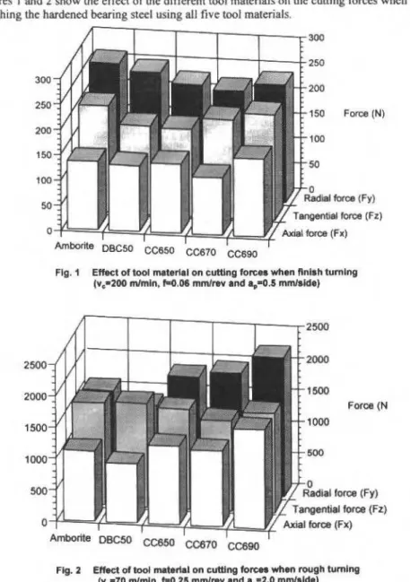
low coocentratlon PCBN compacts and conventional ceramic cutting tools (m.ixed alumina, whisker reinforced alumina and silicon nitride bascd oeramics). The resuJts indicated that in general, the radial force was the highest. foUowed by the J:angcntial and axial forces. When roughing. cutting forces were approximatcly 6-9 times higber than whcn finishing. Cutting forces increased almost Jinearly with feed rate, depth of cut and tool wear, but decreased sligbtly as the cutting speed was increased.
Keywonb; Hardened Steel. CultÜ\g Forces, Macbining. PCBN, Ceramic Tooling.
lntroduction
Conventional wisdom suggests that steels become " difficuiHo-machlne" at hardness values greater than about 300 HY (30-32 HRC). Therefore workpiece materiais above this limit are recommended to be cut near-net shape in the annealed conditíon, heat treated and finally ground to desired dimensions and tolerances. However, tuming and milling such materials using PCBN and ceramic tooling instead of grínding is often quicker and th erefore, substantial cost savi ngs can be made (Collier, 1987). Addítionally, bard part macb ining (HPM) avoíds the problems of distortion and subsequent re-machíning that typically occur with existi ng processing procedures used in die block manufacture.
High-speed steel and cemented carbide tool s are ineffective as their edge strength is insufficient to withstand the cutting stresses at elevated temperatures and diamond reverts to graphite at temperatures above 750°C. The ability of polycrystallíne cubic boron nitride (PCBN) cutting
tools
to maintaín a workable cutting edge at elevated temperature is, to some extent, shared with several of the newer conventíonal ceramic tool materiais, thereby offering an alternativo to PCBN in a number of circumstances.Cutting forces when machining hnrd materiais are not extremely higher than when cutting in the annealed state due to the relatively small amount of plastic deformatioo of the chip (limited by crack initiation and resulting in a saw-tooth type of chip) and also because of the low contact area between chip and too I, which reduces the friction force (Nakayama et ai ., 1988). Nevertheless, cutting forces are reported to be approxímately 30 to 80% hjgher than when machining materiais of lower hardness (Bordui, 1988). Anenlion should therefore be paid to the tool edge preparation, the use ofnegative rake geometry and appropriate nose radii. Despite tbe lower forces obtained when using a sharp edge, a charnfered edge should be employed ín order to distribute the radial force along the edge and improve the edge resistance to failure by fracture, mainly in the case of rough and interrupted cutting. According to Collier ( 1987) and Stier ( 1988), a large comer radius anda large cutting edge angle
X
r also improves tool strenglh. ln general, when machining hardeoed steels with PCBN and conventional ce ramic tooling, Sandvik recommends the use ofa T-land edge preparation ofO. J mm x 20°. Edge hooing isalso recommended for PCBN tools, typical hone radius values ranging from O. I -0.15 mm for heavy roughing operations when machining steel mill rolls, to 0.02-0.05 mm when fioishing (Hatschek. 198 1).
Kônig and Wand ( 1987) reported that during continuous tuming of a bearing steel hardened to 60 HRC using PCBN tooling, the cutting forces decreased with ao increase in cutting speed up to 200 mi mio, after which they remained constant. The tangential aod axial forces were shown to increase almost
CVt1lng Forces As.s.ustnerll when Tumlng Haldeoed Bearing S1eel 354
linearly with deplh-of-cut. Changes io feed rate produced signiticant variation ln axial aod radial forces, however lhe tangential force was less affected. When usi ng mixed alumina cutting tools to machine case hardened steels, the radial force was found to be up to lhree times higber tban when using PCBN tools.
When macbining hardened too! stcels (58 HRC) using DBCSO wlth a positive or neutral rake angle too I, Heath and Dodsworth ( 1987) found tbat tlank wear was accelerated aod unstable cutting conditions were produced. Nakai et ai. ( 1991) reported tbat when machining AISI T4 high speed steel wilh PCBN tools, increasing lhe workpiece hardness from 15 to 62 HRC resulted lo a gradual increase of the tangential and axial forces, but that tbe radial force increased rapidly when lhe workpiece hardness exceeded 45 HRC. Tuming AISI 01 tool steeJ using PCBN tooling (BN200), Ahmad et al. ( 1988) found that an increase in the work material hardness had a profound effect on both the tangential and feed forces due to an increase in the energy necessary to shear the harder material. When comparing lhe radial forces for mixed ceramic and PCBN tools used for turning case hardened DIN 16MnCr5E steel (62 HRC), KOnig e! ai. ( 1990) reported that the míxed ceramic too I produced radial forces two to three úmes higher than with lhe PCBN insert..
As far as the machine too I is concerned, the static and dynamic stiffness of the machine too V workpiece pair are of great importance wheo HPM , sioce vibratlon must be minimised, if not eliminated, during cutting. This can be achieved through a proper design of bed ways as well as headstock and tailstock bearings. When varying the stlffness of tbe machine tooVworkpiece system during hard cutting with PCBN tools, Chryssolouris (1982) found tbat with low stiffness, wear behaviour was characterised by early cracking, leading to a decrease in too I Life. Unfortunately, data on lhe minimum stiffuess required for a satisfactory tool performance are not available.
Although the technicalliterature is not spec ific with regard to lhe power consumption wben HPM, machine tools with a minimum power from I O to 15 kW are generally r equired. Other recommendations include (Ekstedt, 1987): protection ofbed ways from cbips and contaminates., proper lubrication of bearings, bigh accuracy of the vital components of the machine-tool and compensation devices and production systems tbat provide tbe accuracy and repeatability required.
The application of a cutting Ouid is recommended when machining components wbich must attain close tolerances and accuracy. ln these cases, a 5% water soluble oíl emulsion provide acceptable results (Collier, 1987). lf tlood coolant is impracticaJ, the use of a spray mist, refrigerated aír or compressed air is advised.
Experimental Work
Continuous dry turning tests were conducted on a 17 kW Dean, Smith & Grace latbe with a top speed of 2000 rpm wbicb was continuously variable. Bars of AlSl 52100 bearing steel containing 0.95% carbon and L73% chromium (determ ined with a HiJger Polyvac EIOOO spectrometer) were heat treated to provi de a case hardness of 62 ± 1 HRC. Due to tbe fact tba1 tbe dépth of the hardened layer did not exceed I O mm. lhe workpiece hardness was closely monitored throughout the test program with an Encotest ETI I portable hardness tester and rehardening was undertaken when recorded v alues approached thc lower control limit. Cutting forces were measured using a Kistler piezoelectric dynamometer model type 9257 A connected to a bank charge amplifiers and a UV recorder during the
ftrSt 30 seconds of cutting.
355
Results
A. M. Abrto and D. AspinwaJI
Table 1 Tool materiais and geometry
Tool material trade name
Amborite (PCBN) DBC50 (PCBN) CC650 (mlxed alumina)
CC670 (whisker reinforced alumina)
CC690 (silicon nitride based ceramlc)
lndexable insert geometry
SNMN 090316 T02020
SNMN 090316 T02020
SNGN 120416 T02520
SNGN 120416 T01 020
SNGN 120416 T02520
Figures I and 2 show the effect of lhe different tool materiais on tbe cutting forces wbeo fmishing and roughing tbe hardened bearing steel using ali flve too I materiais.
300
250
Force (N)
200
150
100
50
of===f=~~~==~==~
Amborite DBC50 CC650 CC670 CC690
Fig. 1 Effllct of tool material on euttlng forces when flnlsh tumlng
(v~200 mlmln,
r-o.oa
mmlrev and a,•O.S mmlalde}Fig. 2
2000
1500
Force (N
1000 500
Effeet of tool material on euttlng forces when rough tumlng
Cuttlng Foo:ea Assessment when Tumlng ftardened Bearing Steel 356
ln general, the radial (thrust) component was the highest, followed by the tangentíal (cuttlng) force and axial (feed) force. Amborite produced the highest forces during finishing, foUowed by DBC50. The conventional ceramic products gave lower values. When roughing using PCBN-based tools, the tangential force was slightly hlgher than the radial component. No such difference was found with the conventiona.l ceramic tools.
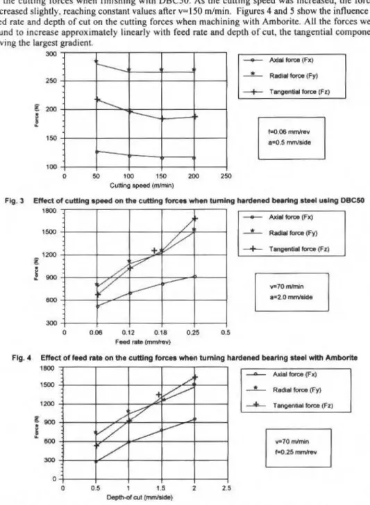
For the subsequeot tests, only the PCBN tools were used. Figure 3 shows the effect of cutting speed on the cutting forces when finishing with DBCSO. As the cutting speed was increased, lhe forces decreased slightly, reaching constant values after v= 150 m/min. Figures 4 and 5 show lhe influence of feed rate and deplh of cut on lhe cutting forces when machining wilh Amborite. Ali the forces were found to increase approximately linearly wílh feed rate and deplh of cut. the tangential component having the largest gradient.
300
..___
g 200 R
"-.
,...__
...
150,._
100
o 50 100 150 Cutllng apeed (m/mln)
200 250
- Axial force (Fx)
-*-
Racll* force (Fy)-+-
TllniJenUIII force (Ft)f:0.06 mm/rev a=0.5 rnrnllllde
Fig. 3 Etfect of cuttlng apeed on tha cuttlng ton:es wtlen tumlng harclened beartng ateei uatng 09C50
1800
1500
1200
g
i
900600
300
o
/,
+
v
//
v
~_/
..----
~v
0.06 0.12 0.18 0.25 0.5
- Axial force (FX) _ L _ Radial force (Fy)
-+-
Tangenhllon:e (Fz)va70mlmln a•2.0 mm/alde
Fig. 4 Effect of feed rate on the euttlng foreea when tumlng harclened beartng ateei wlth Amborlte
1600 1500 1200 300 o o . /
j
~
/ .
~
~
~
v
/
0.5 , 1.5 2
OepCh.ol cut (nvnlllde}
2.5
_..__ Aldal force (Fx)
- *-
Radial force (F'()_.__ T engenllal force (FZ)
357 A. M. Abrflo ando. AspinwaD
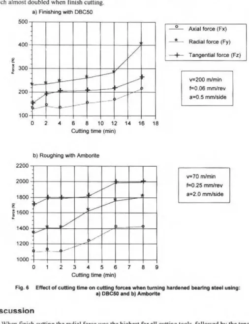
hnally, Fig. 6 shows lhe effect of cutting time, and consequently tool wear on the cuttíng forces, when: a) finish tumíng wíth DBC50 and b) rough tuming with Amborite. The end of thc test was determined by lhe time required for each too! to reach an average flank wear VB8 ... 0.3 mm. Altbough ali lhe forces increased with cutting time, the moSt dramatic change was observed in the radial force, which almost doubled when finish cutting.
500 400 300 200 100 2200 2000 1800 1600 1400 1200 1000
a) Flnishing wtth DBC50
v
/
f----' c---
---f - -
v
f -
-
v
/
~
- --'/...---·
r----
>-_
_,~
o
2 4 6 8 10 12 14 16 18Cuttlng time (min)
b) Roughing wlth Amborlte
v
v
--o
v
/
_....-
I-v
v
v
/
:./---'
v--·-2 3 4 5 6 7 8 9
Cuttlng time (mln)
- 0- Axial force (Fx)
---À...- Radial force (Fy)
-+-
Tangentlal force (Fz}v=200 mlmln
f.=0.06 mmlrev
a=0.5 mmlside
v=70 mlmln
1=0.25 mmlrev
a=2.0 mmlslde
Fig. 6 Effect of euttlng time on euttlng torcaa wtlen tuming tlardaned beartng atHI ualng: a) OBC50 and b) Amborite
Discussion
When finish cutting the radial force was the bighest for ali cutting tools, followed by lhe tangential and then axial force. This was not unexpected, since wheo cutting bardened-~Js the radjal force is
Cutting Forces Assessment wt1en Tumlng Hardened Beartng Steel 358
to its high thennal conductivlty.
By
channelingheat
away from the cutting zone the induced softening of the work material was reduced, thereby giving rise to higher cutting forces. When rough cutting however, two different operating regimes were observed: Amborite and DBC50 gave tangential forces marginally higher than the radial component whereas the conventional ceramic products followed the sarne trend observed when finish tuming. One possible explanation for the bebaviour of Amborite and DBC50 was found examining the pro file of the cutting edges (Abrão, 1995). After only two minutes cutting, the slope of the crater wall was much steeper on the whisker reinforced alurnina and silicon nitride cerarnic tools lhan on Amborite, and lhe crater was located very close to the cutting edge leading to its deterioration. Consequently the radial component ofthe resultant cutring force will be much more promineni compared to Amborite (and possibly to DBC50) where the shape of the crater will lead to a more equal share of the resultant force between the tangentiaJ and radial components. The narrower width of lhe chamfer produced on lhe whisker rcinforced tools was possibly thc maio responsible for the slightly lower resultant cutting force when finish cutting.The decrease in the cutting force as the cutting speed increased was probably caused by a reducrion in the strength ofthe material owing to an increase in the cutting temporature and was also reported by Kõnig and Wand ( 1987). Ali forces increased with feed rate and depth of cut., however the radial force which was the highest at the beginning of the tests (lower feed rate and depth of cut) was overshadowed by the tange ntial force as the cutting parameters were increased. Similar results were reported in the literature by Hodgson and Trendler (I 987) and KOnig and Wand ( 1987) and it would appear that under such conditions. it is likely that the associated increase in temperature was not sufficient to match the increase in the shear plane area and soften the work material.
The effect of the cutting time, and consequently tool wear on cutting forces was investigated wheo finish tuming using DBC50 and when rough tuming with Amborite. As expected. ali thc forces increased with cutting time, especially the radial force when fin ishing which seemed to be more responsive to the wear experienced by the cutting too I.
Conclusions
Cutting forces measurements undertaken when tuming hardened bearing steel indicated that, in general. radial forces were the highest, followed by the tangential and axial components, except when rough cutting using Amborite and DBC50 wbere the tangentíal force was marginally greater, and
The forces were found to docrease slightly with cutting speed and to increase with feed rate, depth of cut and too I wear.
Acknowledgments
We would like to thank Professor K.B . Haley, Head ofthe School ofManufacturing & Mechanical Engineering and Professor M .H. Loretto, Director of the IRC in Materiais for High Performance Applications, for lhe provision of laboratory facílities. AdditionaJ thanks goto Paul Bossom and Shaun Webb, De Beers Industrial Diamond Division (PTY) Ltd., for thc supply of PCBN tooling materiais and both CNPq-Brazil and EPSRC-UK for fmancíal support.
References
Abeto, A.M., 1995, MThe Machining of Annealed and Hardened Steels Using Advanced Ceramic Cutting Tools ~ . PhD. Thesls, University ofBirmingbam, UK.
Ahmad,M.M., Hogan,B., and Goode, E., 1988, "Machinabillty Tests on Cubic Boron Nitride", Proceedings, Fifth Conference of the Irish Manu facturing Committee, Advances ln Manu facturing Technology, pp. 495-S 14. Bordui, D .. 1988, ''Hard-Part Machining With Ceramic lnserts", Ameriean Ceramic Society BuUetin , Vol. 67(6),
pp. 998-1001.
Chryssolouris.O .. 1982, wEffects of Machine-tool-workpiece Stiffness on lhe Wear Behaviow Of Superhard Cuning Material", Annals of theCIRP, Vol. 31(1), pp. 65-69.
359 A. M . AbfAo and o. Asplnwall
Hal ~c h e k . R.l... 1981 , "Take a New t.ook AI Ceramic/cermets". American Machinist. Special report no.:733, pp. 165-176.
Hcath, P.J. and DODSWORTH.J. 1987. "Brazeable PCBN lnserts-a Usc:r's Guide".lndustrial Díamond Review. Vol 3. pp. 107-111
Hodg.son. T. and Trcndlcr, PJ UI., 1980, ··cubic Boron Nilridc Machinjng; With Particular Referenoc to Cutting Tool Geometry and Cutting Force$ When Machining Tool Steer'. Proceed ings, l ntcmationaJ Confcrence on Manufacturing Tcchnology, pp. 63-70. Melbourne, Austral ia.
Konig, W., lding, M .. and Link, R. , 1990. ~ Fine Tuming and Drilling Hardened Steels", Industri al Diamond Review, Vol. 2, pp. 79 • 85.
Kõnig, W., and Wand , Th., 1987. ~T urnlng Bearing Steel Wlth Amborite and Ceramic", Industrial Diamond Review. Vo1.3.pp. ll7-120.
"\aklli.T., Naklltani,S .,Tomita. K., and Goto, M., 1991, " Hard Tuming by PCBN", Proceedings, Superabrasivcs'91, SME. pp 1161-1175. Chicago. I L. USA.
Nakayama. K .. Arai. M .. and Kanda. T., 1988, " Machiniog Characteristics ofHard Materiais", Annals ofthe CIRP, Vol. 37(1 ). pp. 89 · 92.
!\ 1-l Sandvik Coromant Hard part lUming guidc, 2 1 p.
RBCM • J. of lhe Braz.. Soe. Mecbanlcal Sclencn
V o/. XVII • n•4 • 1 !195 • pp. 360-372
ISSH 0100-73$
Printed ln Brazll
Comparação de Métodos Estacionários e
GMRES em Simulação de Reservatórios de
Petróleo Utilizando Malhas Não-Estruturadas
de Voronoi
Comparison of
some Estationary Methods with the GMRES
in the Petroleum Reservoir Símulation Using
Non-Structured Voronoi Grids
Francisco Marc:ondes
Universidade Federal ela Paralba Departamento de Engenharia Mecênlca Campina Grande. PB Brasil
Mário Cesar Zambaldl
Univef'Sldade Federal de Santa Catarina Departamento de Matemática 80040-900 Florfan6polis, SC Brasil
Clovis Raimundo Mallska
Univef'Sldade Federal de Santa Catarina Departamento de Engenharia Mecênlca 88040..900 Florianópolis,
se
BrasilAbstract
The solution of lhe linear systcms arising in pc:troleum reservoir engineering simulatlon using non-sttuctured Voronoi grids is the main goal ofthis work. Thc solutloo is obcained using stationary and GMRES (Gcnctalized Minimal Residual Method). The GMRES mcthod is preoonditioned by two schem.es: ooc of thcm is based on a ILU factorization while thc other one takes into account only ofthe jacobian matrix struetured.
Two ordering schemes, are also investigated, one is based oo the grid generatlon structure and lhe other one via ordering planes.
Krywords: Petroleum Reservoir Simulation, Noo-structuTed Voronoi Orids, Stationary Met.hod, OMRES, Natural Grid Generaúon, Ordering Planes
Resumo
No presente trabalho a soluçllo dos sistemas lineares oriundos da simuJaçllo de reservatórios de petróleo utilizando malhas não-estruturadas de Voronoi é obtida através de métodos estacionários e GMRES (Generalized Minimal Residual Met.hod). Para a resoluçlo oom o método GMRES
sao
utilizados dois tipos de ~ndicionadores. um global e outro baseado somente em uma parte da estrutura do jacobino.Também, são utilizados dois esquemas de ordenaçllo das incógnitas, uma baseada na geraçllo natural da malha e outra via plano ordenador.
Palavras-cllan( SlmulaçAo de Reservatórios de Petróleo, Malhas de Voronoi, Métodos Estacionários, GMRES, Geraç1o Natural da Malha, Plano Ordenador.
Introdução
A simulação numérica de reservatórios de petróleo é uma ferramenta de importância vital no auxllio do gerenciamento de uma determinada bacia petroHfera. O primeiro passo na simulação é a escolha de um modelo matemático que represente adequadamente o comportamento dos fluidos presentes no reservatório. Em geral, por mais simples que seja o modelo, as equações representativas sao altamente não-lineares e acopladas. Com o intuito de obter as equações aproximadas estas equações
sao
integradas no espaço e no tempo. Para a integração temporal, geralmente é utilizado um esquema totalmente impllcito no tempo e o conjunto de equações não-l ineares 6 resolvido utilizandoiteração de Newton.
Para a discretização do domlnio espacial existem diversas possibilidades, as quais podem-se englobar dentro de duas categorias básicas, malhas estruturadas e malhas não estruturadas. A malha
361 F. Marcondes, M. C. Zambaldl and C. R. Mallaka
estruturada mais utilizada na simulação de reservatórios de petróleo é a malha cartesiana (Yanosik e McCraken, 1983; Rubin c Blunt; 1991; etc). Recentemente apareceram trabalhos que fazem uso de coordenadas curvillneas (Fieming, 1987; Sharpe, 1993; Maliska et ai .. 1993), sendo que os dois primeiros trabalhos citados trabalham com coordenadas curvillneas ortogonais e o último com coordenadas curvillneas nAo-ortogonais.
Em malhas não-estruturadas existem trabalhos que fazem uso da técnica dos elementos finitos (Coutinho et ai. , 1993) e aqueles que fazem uso de malhas não estruturadas, mas continuam realizando balanço de massa para cada componente (Forsyth, 1989; Fung et ai., 1993; Palagi, 1992). A malha proposta por Palagi ( 1982) é um caso partic!Jlar dos trabalhos de Forsyth (1989) e Fung et ai. (1 993), uma vez que a malha utilizada pelo mesmo é um diagrama de Voronoi. cuja principal caracterlstica é ser localmente ortogonal. Isso, por sua vez. facilita sobremaneira o processo de integração das equações governantes.
A grande vantagem do uso de malhas não-estruturadas, no que tange a discretização do domínio é a facilidade de representar geometrias bastante complexas. Trabalhando-se com malhas estruturadas nem sempre é possivel resolver um determinado problema sem que se tenha de fazer uso de vários domlnios, mesmo trabalhando-se com coordenadas generalizadas. Entretanto, o sistema de equações resultante , quando do uso de malhas não estruturadas, é geralmente esparso e sem nenhuma lei de formação, o que influencia o método numérico para a resolução do problema.
Para a resolução do problema, utiliza-se iterações newtonianas em cada nfvel de tempo. Em cada interação de Newton um sistema de equações lineares deve ser resolvido. Métodos iterativos devem ser empregados para os sistemas lineares, como a literatura do petróleo s ugere. Isto porque os métodos iterativos requerem, em geral, pouca memória adicional e baixo custo por iteração.
A ordenação das incógnitas afcta a taxa de convergetlcia dos métodos baseados ou derivados dos gradientes conjugados precondicionados para malhas estruturadas (Watts, 198 1; Behie e Forsyth, 1984 ). No caso de malhas estruturadas as matrizes, apesar de serem esparsas, têm uma lei de formaçao. por exemplo, cinco diagonais para problemas bidimensionais. Conforme O' Azevedo et ai. ( 1991) a combinação de malhas nilo-estruturadas com meios bastante heterogêneos, tomam os métodos, que trabalham com algum esquema de precondicionamento baseado em fatoraçllo incompleta, bastante sensfvel à numeração dos nós. Em muitos casos não existe uma maneira óbvia de ordenação. Evidentemente, este problema nll.o é grave quando se trabalha com métodos não-precondicionados. A qualidade do precondicionador influenc ia muito na taxa de convergên~ia do método iterativo e a ordenação dos nós influencia diretamente o precondicionador.
Os métodos ponto a ponto requerem pouca memória adicional e tem custo reduzido por íteraçllo. Por outro lado, a taxa de convergência é lenta quando comparadas aos métodos não-estacionários, e geralmente dependem de parâmetros a serem definidos pelo usuário. Este fato é significativo pois além de considerar muitas iterações no tempo, também são necessárias várias iterações newtonianas para um intervalo de tempo.
No presente trabalho, será dado ênfase à solução dos sistemas provenientes da simulação numérica de reservatórios de petróleo utilizando malhas de Voronoi. A geração da malha de Voronoi é obtida pelo gerador desenvolvido por Maliska Jr. (I 993). O modelo utilizado é o Black-Oil, bifásico e a análise será restrita a geometrias bidimensionais. Na resoluçao dos sistemas lineares oriundos da linearização de Newton serão abordados os métodos ponto a ponto de Jacobi, Gauss-Seidel e SOR (Sucessive Over-Relation), e o método GMRES. Serão testados dois tipos de precondicionamento neste trabalho. O primeiro é um tipo de fatoraçâo incompleta simplificada, baseada na concentraç!lo dos elementos próximos à diagonal, e o outro é uma fatoraç!lo que leva em consideração toda a estrutura da matriz. Na solução com o GMRES serão investigados dois esquemas de ordenaçll.o. Um oriundo da geração natural da malha, e outro, obtido por uma ordenação semelhante à utilizada para malhas cartesianas.
Descrição dos Métodos
De acordo com a formulação do problema, deve-se resolver um sistema linear newtoniano várias vezes, mesmo numa simples iteração de Newton. Considere, entao, o sistema linear de n variáveis,
Comparison of Some Estationary Mettlods with lhe GMRES ln lhe ... 362
onde
J
v é a matriz jacobiana e fv é a função reslduo na v-ésima iteração de Newton, num passo arbitrário de tempo.Os sistemas lineares da Eq. ( I ) devem ser resolvidos. aproximadamente, por métodos iterativos lineares. Um critério de convergência baseado em considerações teóricas e práticas dos métodos de Newton lnexatos (Dembo et ai., 1982), deve ser
(2)
onde
e -
O, . Os métodos iterativos originalmente apresentam taxa de convergência lenta e precisam ser acelerados. Isto caracteriza o uso de precondicionadores, (Golub e Van Loan, 1989). Teoricamente, funcionam como se fosse aplicado o método iterativo no sistema linear equivalente, porém mais fâcil de resolver,(3)
onde M é chamada matriz de precondicionamento. Esta matriz deve ser ao mesmo tempo uma aproximação para o Jacobiano e sua açllo sobre um vetor. simples de calcular. Efetivamente, o sistema da Eq. (3) nào é explicitado e aplica-se o precondicionador adequando-o ao método iterativo línear.
Os métodos iterativos estacionários ponto a ponto (Jacobi. Gauss--Seidel e SOR) envolvem baixo custo por iteraç!o. Por outro lado, a tax.a de convergência é lenta, além de restrições sobre a matriz Jacobiana (dominância diagonal) e da dependência de parâmetros, como no caso do SOR. Com filosofia oposta. os métodos iterativos nllo~estacionários envolvem uma minimizaçllo de funcional, que é quadrático. simétrico e positivo definido para o gradiente conjugado (GC) clássico, restrição eSta que é relaxada no GMRES desenvolvido por Saad e Schultz ( 1986). Considere, para maior clareza da descrição dos métodos que serao apresentados, o sistema linear da Eq. ( I), sem indexação da iteração de Newton.
JAX = f (4)
Métodos Iterativos Estacionários
Os métodos dessa natureza são baseados, no processo iterativo
(5)
onde o "sobrescrito" K significa agora a K-ésima iteração do método iterativo, numa determinada iteração newtoniana
A matriz do sistema linear é particionada da forma J= B-N. Para o processo iterativo da Eq., (5), o sistema linear em B deve ser simplificado. A condição teórica de convergência do processo da Eq .. (5) é que o raio espectral da matriz 8 '1N seja estritamente menor que I (um). Para descrição dos métodos
na forma matricial, suponha J= L+(}+.U, onde D= Diag (1), L eU as partições estritamente tri.angular inferior e superior, respectivamente, da matriz J.
Um esquema simples para a Eq., (5) é o método da Jacobi, onde B= D, N= -(L+U). Em forma de componentes do vetor solução pode-se escrever,
[
i - 1 n )
t.X.(k+l ) o: f. - ~ J .. t.X.(kl _ ~ J .. t.XJ(k )
/J ..
I I ~ 1) ) ~ IJ 11
j -I j • i-+ I
363 F. Marcondes, M. C . Zambaldl and c. R. Maliska
No método SOR, utiliza-se a informação atua1izadajá dispoolvel dos componentes t.Xi<k • t) _ Além disso introduz·s~ no particionamento, um parâmetro de relaxa~o da forma B=D+ a L e N={
l-a )D-U. O parâmetro aE (0,2) deve minimizar o raio espectral de B- (a) N (a) . Observe que se a
= I tem-se o método de Gauss-Seidel. Pode-se escrever então,
[
i -I n
l
t..x .(lc · 1l "'" a
r.- ""
JJt..x.<k - ll - "" J .. t..x .<kl /J .. + < 1 - a)t..X.<klI I "-' I J .LJ IJ J 11 I
j=l j • i+l
(7)
o desempenho da iteração SOR depende da escolha de a e, na maioria dos problemas, é imposslvel obtê-la sem uma anâlise da distribuição dos autovalores de B·1N.
Em muitos casos, a matriz jacobiana apresenta estrutura de blocos. Suponha que J ij seja uma submatriz njxn1 e n1 + n2 + --- + n'L ~ n, a dimensl!.o do sistema do linear. Nesse caso t..X. e f. representam subvetores de ordem n1. tnUio, para o processo iterativo do método de Gauss-Sei dá po~
exemplo, tem-se
t..x
1<k • 11 = [ f ... I
i~l
.LJ j. t.X IJ J <k • 11 _~
"-' j .. lj f.X <kl Jl/J.
11 J • I J • i + 1(8)
No presente trabalho, a matriz jacobiana é de blocos, com cada bloco sendo de dimensão 2.
Método GMRES
O GMRES faz parte de uma classe de métodos (ORTHOMIN, ORTHODlR, ORTHORES, GCR) obtidos por generalização do gradiente conjugado. O residuo corrente, r • f - Jt..X , é minimizado no
• O O 2 O m - 1 O
o
subespaço de Krylov asso<: lado ao sistema, K m = span {r , Jr . J r . ~ J r } , onde r é o resfduo no ponto inicial. Para tal. é necessário obter uma base ortonormal de Km. através do processo de Gram-Schimdt modificado e, posteriormente, resolver um sistema triangular, cujos elementos sào gerados durante a onogonalização. F,.sse sistema reduzido tem a dimensl!.o do parâmetro de recomeços da onogonalização, uma vez que, por limitação de memória e do custo-iteração, a base do subespaço Km não pode ser e~tendida arbitrariamente. Fica caracterizado. no contexto do método, a resolução de um problema de quadrados mínimos associados. o que permite evitar o denominado "break-down" no contexto de Lancws (Golub e Van Loan, 1989), suscetlvel a outros métodos dessa classe. O algoritmo do método, na versão de recomeços a cada m iterações. é descrito a seguir, onde a matriz de precondicionamento
M.
é dada por fatoraçào incompleta.ALGORiTMO GMRES (m). Dado o vetor aproximação t..x0 e a matriz de precondicionamento
M. faça
passo I -inicialização
r0 "' M -1 (f-Mx0) e v1 = r0
/~r
01!
passo 2 - ortogooalizaçãoparaj= l, ... ,m
Cornparison of Some &tationary Melhods wíth lhe GMRES in lhe ...
W+-w -
L
uij vii - 1 uj + lj =
llwll
. +I
v
=
w / u j+ljpasso 3 - solução corrente
passo 4 -recomeço
se
llr
0ll
< TOL pare senãoO m I m R mil
ôX = ôX e v = r /ur u
No algoritmo acima. e 1 é o veto r canO nico de o+ I componentes, Um é uma matriz de ordem (m+ I )xm do tipo Hessemberg, obtida pelos uij• V m é uma matriz nxm , cujas colunas são os vetores vi e TOL é a tolerância para convergência. Na implementaç!o computacional é possfvel executar os passos 2 e 3 simultaneamente por rotações de Givens. Neste caso, a norma do reslduo fica sempre disponlvel na j-ésima iteração. onde o teste de convergência é feito, sem explicitar a solução.
Fatoração Incompleta (ILU)
Os esquemas de precondicionamento baseados em fatoração incomple.ta (ILU- lncomplete LU factorization), consistem em obter fatores M=LU na forma produto, onde L é triangular inferior unitária e U é triangular superior, considerando estruturas que não perm1tem excessivo preenchimento nas matrizes de L e U, o que normalmente ocorreria na fatoração completa do jacobiano.
A matriz de precondicionamento deve ser uma boa aproxim.ação da matrizjacobiana (M-J), e deve ser fácil de fatorar. Existem diversas possibilidades na fatoraçllo de M. Uma forma posslvel é tomar M como sendo a diagonal de J. Neste caso, o cálculo da inversa de M é direto. No presente trabalho usar-se-á dois tipos de precondJcionamento.
365 F. Marcondes. M. C. Zambaldt and C. R. Mallska
{
O se ) ..
~O
I (J .. ) c IJ
'J - se J .. IJ =O (9)
No m-~ s imo passo da eliminação gaussiana. defini-se
t(J .) = minlt(J),t(J ) +t(J . ) + I)
IJ IJ tm nlJ ( lO)
Todo~ os elementos nos fatores LU de J têm nível O. Se uma fatoraçào incompleta de nlvel I é realizada somente os elementos com ordem menor ou igual a um são aceitos. com os elementos de ordem mais alta sendo rejeitados. Quanto maior o nlvel da rLU, menor o custo por iteração do método iterativo. entretanto. a memória e o trabalho na realização da fatoraçllo aumentam, o que pode comprometer o desempenho global.
Modelo Fisíco
O s resultados que serão apresentados foram oriundas da simu laçllo numérica do escoamento bifàsico (ó lco-âgua) em reservatórios de petróleo. A seguir serâ apresentada uma breve descrição do modelo. Assumindo que existe somente duas fases imisciveis no reservatório (óleo (0) e ãgua (W)) e desprezando os efeitos de pressão capilar c gravitacional, pode-se escrever a equação de conservação volumétrica para a fase p como.
(li)
onde ~ é a porosidade e BP é o fator de formação volumétrica da fase p. SP é a saturação da fase p, Pé a pressão dos nuidos presentes no reservatório e qP é a razão nas condições de armazenamento da fase p por unidade de volume do rese.rvatório e ÀP é a mobilidade da fase p, dcftnida por
( 12)
onde K é a permeabilidade absoluta do meio. ~a permeabilidade relativa e ~P a viscosjdade, da fase p.
Escrevendo a Eq. ( 11) para a.~ fases óleo e ãgua constata-se que existem três incognitas (S0, Sw e P)
e ape nas duas equações. A equação para o fechamento do problema vem da conservação da massa global. dada por
( 13)
Integração das Equações Governantes
A Fig. I apresenta um volume de controle de Voronoi. O ponto i é o gerador e os pontos j's seus vizinhos. Para cada ponto j é possfvel a linhar um s istema cartesiano local x' -y' de tal forma que o eixo x · (linha que une o ponto i ao ponto j) seja perpendicular à face do volume de controle e o eixo y'
Comparison of Some Estatlonaty Methods w!tt1 lhe GMRES lo lhe ...
j=2 ~
I
•
j=4
ijp "'
Fig. 1 Volume de controle de Voronol
Integrando a Equações (li) no espaço e no tempo, tem-se
(.t.V Sn)"+ '-(.t.V S")n
:Z:...:...L :Z:...:...L=
~T N. .. ),n~.l(pn + l _ pn ~ l)+qn + l Ál BP i Ál BP i Li 1J p, 1J p.j p, 1 pj =I
•
j=S(14)
A Eq. ( 14) mostra que a metodologia empregada é totalmente implfcita, uma vez que nesta equação existem termos (mobilidades e fator volumétrico, por exemplo, que dependem das incógnit_aS do problema (Sp e P).
llp
é a vazio volumétrica da fase p nas condições de superflcie e Nv o número de vizinhos do volume i. O termo T;i na Eq. ( 14) é conhecido como fator de transmissibilidade e é o produto de fatores geométricos e da permeabilidade absoluta, dado por(15)
onde h e b são a altura e largura da face ij, respectivamente.
O sistema de equações é resolvido iterativamente usando o método de Newton. A forma residual da equação de conservação do componente p para o volume i é
N. ( K )" + I ( V S
)n
+ I R . =L
T . -.-!2.. (P!I + I _ P!l + I) + qn + I _~
...2 ·-p, t IJ ~PBP ij J 1 p .ó.t BP IJ • I
+(~~)"o
p= o wÁt BP i • •
(16)
Expandindo o reslduo em série de Taylor, tem-se
(17)
367 F. Marc:ondes. M. C. Zambaldi and C. R Maliska
~ (~)v
v+l
L
ax
t.X = - R;;;p =o,w V'XAs incógnitas (P e Sw) são calculadas, após cada iteração newtoniana. como
e a solução é aceita quando todas as tolerifldas são satisfeitas, de acordo com
ó.P~. ~~x ~ ó.Po~ max
ASV + I <AS*
u w. max - U w, max
Resultados
( 18)
( 19)
(20)
Os resultados que serão a seguir apresentados foram obtidos com o GMRES e Gauss-Seidel (GS). Foram realizados, também, alguns testes com o Jacobi e SOR. Entretanto, os resultados obtidos com os mesmos não serão aqui apresentados por diversas razOes. Foi constatado no decorrer dos testes com o método de Jacobi que os erros de balanço de componentes eram sempre superiores ao GS. Como a estrutura numérica da sequência de sistemas são distintas, mesmo em cada iteração newtoniana, valores diferentes de ex podem ser necessários para o SOR. Tentativa de obtenção de uma estimativa razoável deste parâmetro em alguns nlveis de. tempo nlo apresentaram converg~ncia. Verificou-se, também, que a taxa de convergência do método de GS podia ser melhorada se a estimativa inicial fosse dada pela solução do sistema Jbt.X = f, onde Jb é a diagonal da matr iz jacobiana. Este foi a estimativa inicial para todos os testes realizados com o método de GS. Isto caracteriza um tipo de precondicionamento por estimativa inicial. Deve-se salientar que o precondiclonamento explicito para os métodos ponto a ponto não permitem uma fórmula dada pela Eq. (8). De fato, neste caso exigiria explicitar a matriz M'1 J e, posteriormente, efetuar a partição em somas de fatores, o que é
evidentemente inviável para uma fatoração incompleta usual.
Para os resultados obtidos com o GMRES foram utilizadas duas ordenaçOes. Uma ordenação da geração natural da malha e outra através de uma linha ordenadora horizontal ou vertical. Considere-se, por exemplo, o caso de uma linha horizontal. Localiza-se o ponto gerador com o menor valor de y e passa-se uma linha horizontal com altura igual a y minimo. Todos os pontos geradores que estiverem sobre esta linha serão renumerados. A seguir, localiza-se entre os pontos nlo renumerados. o próximo ponto com menor valor de y c repete-se o processo anterior. Este processo 6 feito at6 que todos os pontos sejam renumerados.
Para todos os casos que serâo apresentados. o máximo ót para o GS e GMRES foram diferentes. Foram feitas algumas experi~ncias e verificou-se que o GS conseguia trabalhar bem com um t.t
máximo de 18.600 segundos. Para o GMRES trabalhou-se com 36.000 segundos. Apesar de ter-se permitido avançar a solução com intervalos de tempo bastante grandes, foram realizados alguns testes com Ât reduzidos pela metade para verificar se o transiente flsico estava sendo respeitado. Apesar de não reportado neste trabalho. a concordância foi excelente. Todos os testes foram realizados numa estação de trabalho Sun SPARC Station 10 com placa processadora P512. Foi utilizado como critério de parada de uma iteração newtoniana 6,893xl0 Papara ó.Pô.mu e J0·4 paraó.S:,. max ·
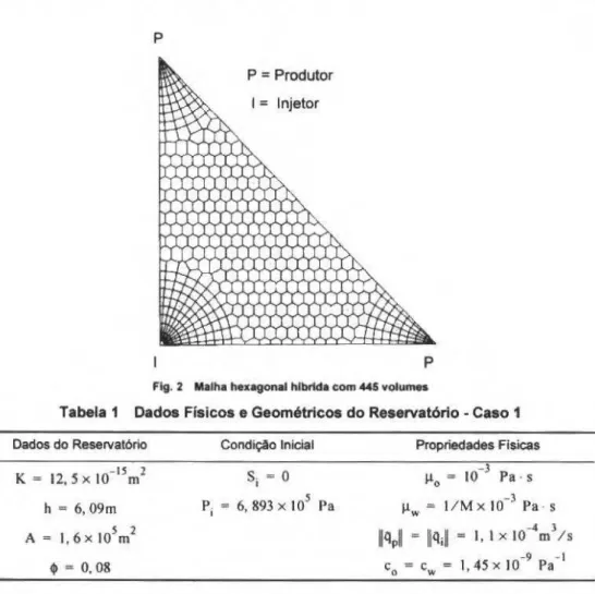
A Fig. 2 apresenta a malha hexagonal hibrida para a configuraçAo de cinco ~os . A Tabela I apresenta os dados 11sicos e geométricos para este caso. As curvas de permeabilidade relativa silo dadas pela Eq. (21):
K =
s
2rw w
2 K,ro .. ( I - Sw)
M = llo/ J.lw
Comparison ot Some Estatlonary Methods wíth the GMRES in lhe ...
p
P =Produtor I= lnjetor
p
Fig. 2 MaJha heJtagonal hlbrida eom 445 volumn
Tabela 1 Dados Flsicos e Geométricos do Reservatório -Caso 1
Dados do Reservatório
K = 12,5 x l0-15m2
h = 6, 09m A= 1, 6x 10sm2
~
=
0,08CondiçAo Inicial
S; =O
5
Pi = 6, 893 X 10 Pa
Propriedades Fisicas
- .l j.L
0 = lO Pa · s -3 J..lw
=
1/ Mx 10 Pa · s-4 l
lllpl
-= ~ ll; l""
I, I X 10 m /s-9 - 1 c0 = cw=l,45x l0 Pa
368
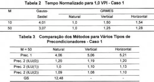
A Tabela 2 apresenta os tempos normalizados para duas razOes de viscosidade. M=IO e M=50, para wn tempo fmal de simulação de 1,0 volume poroso injetado (VPU). Como precondicionamento para o método GMRES foi empregado a parte tridiagonal da matriz jacobiana (prec. I). O tempo normalizado é obtido dividindo-se o tempo de computaçllo pelo tempo de computação mfnimo, de todos os métodos, para cada razão de viscosidade. Pode-se observar o desempenho bastante superior do GMRES para as duas razões de v iscosidade. Um dos motivos deste comportamento é que o GMRES permite trabalhar com intervalos de tempo maiores, e o número de iterações do GMRES foi muito inferior às iterações do GS, apesar do custo da iteração individual do OMRES ser superior. Além disso, pode-se verificar que, com Intervalos de tempo iguais, o desempenho do GMRES seria
ainda superior. Observando-se somente os resultados do GMRES, verifica-se que a ordenação natural
foi a que apresentou melhor resultado. Isto deve-se ao fato do precondicionador utilizado nll.o ser sensfvel às ordenações utilizadas.
369 F. Marcondes, M. C. Zambaldi and C. R. Maliska
Tabela 2 Tempo Normalizado para 1,0
VPI-
Caso 1M Gauss- GRMES
Seidel Natural Vertical Horizontal
10 4,01 1,0 1,50 1,54
50 3,07 1,0 1,25 1.28
Tabela 3 Comparaçlo dos Métodos para Vários Tipos de Precondlclonadores • Caso 1
M=50 Natural Vertical Horizontal
Prec. 1 4,06 5,06 5,21
Prec. 2 (ILU(O)) 1,20 1,19 1,20
Prec. 2 (ILU(1)) 1,0 1,10 1,13
Prec. 2 (ILU(2)) 1,09 1,08 1,10
GS 12.48
A Tabela 4 apresenta os dados flsicos para a malha mostrada na Fig. 3. Neste problema existem 8 (oito) poços, sendo 6 (seis) produtores e 2 (dois) injetores. As curvas de penneabilidade e viscosidade são dadas na Eq. (22}, com as unidades no SI.
K,w = (S - 0,2) (-250S2+32S - 55) Kko = 1-k,w
~w ~
10-3(1+
1,4Ç12P- (l.37 x 107))~o =
I, 1163 x 10-1 (I+ I, 4Ç12P - ( I, 37 x 107))Fig. 3 Malha htx.gonal hlbrtda com 1026 volumtt