Detecção e localização de distúrbios transitórios em linhas de transmissão de energia utilizando sensores sem fio

(1)

Universidade Federal de Minas Gerais

Escola de Engenharia

Programa de Pós-Graduação em Engenharia Elétrica

Detecção e Localização de Distúrbios Transitórios

em Linhas de Transmissão de Energia Utilizando

Sensores sem Fio

Dênio Teixeira Silva

Tese de Doutorado apresentada ao

Programa de Pós-Graduação em

Engenharia Elétrica da Universidade Federal de Minas Gerais, como requisito parcial para obtenção do título de Doutor em Engenharia Elétrica.

Orientador: Prof. Dr. Julio Cezar David de Melo (UFMG)

Co-Orientador: Prof. Dr. José Luiz Silvino (UFMG)

(2)

(3)

Universidade Federal de Minas Gerais

Escola de Engenharia

Programa de Pós-Graduação em Engenharia Elétrica

Detection and Location of Transient Disturbances

in Power Transmission Lines Using Wireless

Sensors

Dênio Teixeira Silva

Thesis presented to the Graduate Program in Electrical Engineering of the Federal University of Minas Gerais in partial fulfillment of the requirements for the degree of Doctor in Electrical Engineering.

Advisor: Prof. Dr. Julio Cezar David de Melo (UFMG)

Co-Advisor: Prof. Dr. José Luiz Silvino (UFMG)

(4)

(5)

(6)

(7)

(8)

(9)

Agradecimentos

Agradeço à minha mulher Leila e aos meus filhos Raphael e Bárbara pelo apoio e paciência,

(10)

(11)

i

Resumo

Este trabalho apresenta uma aplicação de sensores sem fio em linhas de transmissão de energia para detectar e localizar distúrbios transitórios impulsivos causados por descargas atmosféricas diretas na linha e circuitos nas fases. As descargas diretas e os curtos-circuitos produzem correntes transitórias de grande magnitude e com alta taxa de variação de corrente. A corrente de retorno da descarga atmosférica que atinge diretamente o cabo pára-raios circula através do cabo e das torres em direção ao solo. O curto-circuito produz uma corrente transitória que induz uma tensão significativa no cabo pára-raios. Da mesma forma, a descarga direta na fase induz uma tensão significativa no cabo pára-raios. A tensão induzida no cabo pára-raios produz uma corrente transitória com alto valor de pico que circula através do cabo pára-raios e nas torres em direção ao solo. Sensores sem fio, instalados no topo das torres, podem medir essas correntes. A componente transitória das correntes é maior nas torres próximas ao ponto onde ocorreu a descarga direta ou o curto-circuito. Esse comportamento é utilizado para localizar o distúrbio transiente. Cada sensor mede o pico de corrente transitória e o pico da taxa de variação da corrente que circula nas torres. Somente os sensores próximos ao distúrbio medem valores significativos de corrente nas torres. Essas medidas são digitalizadas pelos sensores e enviadas através de uma rede sem fio para um computador de localização. Nesse computador, essas medidas são analisadas através de um programa de localização para identificar se o distúrbio transitório é uma descarga direta ou um curto, para localizar o vão onde ocorreu o distúrbio transitório, e para avaliar a potência no caso de uma descarga direta.

(12)

(13)

iii

Abstract

This work presents an application of wireless sensors in power transmission lines to detect and locate impulsive transient disturbances caused by direct lightning strokes to the line and short circuits. Direct stroke and short circuit on phases produce transient currents of great magnitude and high rate of change. The return current of the lightning stroke to shield wire flows through the wire and through the towers to earth and a short-circuit produces a transient current that induces a significant voltage along the shield wire. Accordingly, a direct stroke to phase cable induces a significant voltage in the shield wire. This induced voltage produces a current with high peak value that flows though the wire and through the towers to earth. Wireless sensors installed on top of the towers, can measure these currents flowing in the towers. The transient component of the currents is greater in the towers close to the stroke or to the position of the short-circuit. This behavior is used to locate the transient disturbance. Each sensor measures the peak value of the transient current, and the peak value of the rate of change of current, but only the sensors close to the disturbance measure significant values of the current in the shield wires. These analog measurements are converted into binary data by the sensors and sent via a wireless network to a computer. In this computer, the values of the measurements are analyzed by the location software to identify whether the transient disturbance is a direct stroke or a short-circuit, to locate the span where the transient disturbance occurred, and to evaluate the power in case of a direct stroke.

(14)

(15)

v

Abbreviations

AC Alternating Current

ANATEL Agência Nacional de Telecomunicações ( National Telecommunications Agency)

AODV Ad hoc On Demand Distance Vector

ATP Alternative Transient Program

CEMIG Companhia Energética de Minas Gerais

CSMA/CA Carrier Sense Multiple Access with Collision Avoidance

CT Current Transformer

CTS Clear-to-Send

DC Direct Current

DCF Distributed Coordination Function

DIFS Distributed Interframe Space

DSDV Destination-Sequence Distance Vector

DSR Dynamic Source Routing protocol

DSSS Direct Sequence Spread Spectrum

DYMO Dynamic MANET On-demand

EMC Electromagnetic Compatibility

EPRI Electric Power Research Institute

FH Frequency Hopping

FTP File Transfer Protocol

GPS Global Positioning System

HTR Hierarchical Tree Routing

HTTP Hyper Text Transfer Protocol

HWMP Hybrid Wireless Mesh Protocol

IEEE Institute of Electrical and Electronics Engineers

IETF Internet Engineering Task Force

IP Internet Protocol

ISM Industrial, Scientific and Medical

ITU-R International Telecommunication Union - Radio Communication Sector

LAN Local Area Networks

(20)

x

LLC Logical Link Control

LLS Lightning Location System

LOS Line of Sight

MAC Media Access Control

MANETs Mobile Ad hoc NETworks

MSC Message Sequence Chart

MTBF Mean Time Between Failures

NAV Network Allocation Vector

NS Network Simulator

OLSR Optimized Link State Routing

OPGW Optic Ground Wire

OPTL overhead power transmission lines

OSI Open Systems Interconnection

PAN Wireless Personal Area Network

PDU Protocol Data Unit

PV PhotoVoltaic

RREP Route Reply Packet

RREQ Route Request Packet

RTS Request-to-Send

SDL System Description Language

SIFS Short Interframe Space

SMTP Simple Mail Transfer Protocol

SNR Signal-to-Noise Ratio

TCP Transmission Control Protocol

TORA Temporally-Ordered Routing Algorithm

TTL Time to Live

UDP User Datagram Protocol

VPN Virtual Private Network

WAN Wide Area Networks

WLAN Wireless LAN

WMAN Wireless Metropolitan Area Network

(21)

xi

List of Figures

Figure 2.1 - Return stroke current measured at Morro do Cachimbo research station. ... 7

Figure 2.2 - Tower with shield wires. ... 8

Figure 2.3 - Lightning location system (LLS)... 9

Figure 2.4 - Direction finder antenna, B is the magnetic flux generated by the lightning, is the angle between coil direction and the hit position. ... 10

Figure 2.5 - Two terminal impedance-based fault location method. ... 11

Figure 2.6 - Two terminal travelling waves fault location method. ... 12

Figure 2.7 - Measurement of current using Rogowski coil, i(t) is the current being measured, v(t) is the coil voltage, and K is a constant. ... 14

Figure 2.8 - The OSI model . ... 16

Figure 2.9 - Internet communication layers. ... 18

Figure 2.10 - The types of information formats and the flow of information between the layers. ... 19

Figure 2.11 - Stack of IEEE 802.x standards . ... 22

Figure 2.12 - 802.11 and 802.15.4 services. ... 22

Figure 2.13 - ZigBee layers . ... 23

Figure 2.14 - Basic access mechanism . ... 24

Figure 2.15 - The problem of the hidden terminal (B) . ... 25

Figure 2.16 - RTS/CTS mechanism . ... 26

Figure 2.17 - 802.11 channels . ... 27

Figure 2.18 - 802.15.4 channels . ... 27

Figure 2.19 - Network topologies. ... 28

Figure 2.20 - Nearly linear topology and the equivalent mesh topology. ... 29

Figure 2.21 - Infra-structured wireless network. ... 30

Figure 2.22 - Infra-structured wireless network. ... 30

Figure 2.23 - Some common Ad Hoc routing protocols. ... 31

Figure 2.24 - The operation of the AODV protocol . ... 33

Figure 2.25 - The first Fresnel zone. ... 35

Figure 2.26 - The elevation angle of the antenna and the difference in the tower levels. ... 37

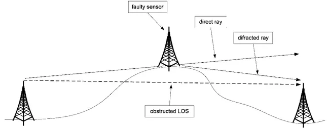
Figure 2.27 - Obstruction of the signal in case of a failure one sensor on the top a hill. ... 38

Figure 2.28 - Dipole antenna ... 38

(22)

xii

Figure 2.30 - Some types of collinear antennas. ... 40 Figure 2.31 - Irradiation diagrams of the collinear array of three dipole antennas . ... 40 Figure 3.1 - Direct lightning stroke currents, i1 an i2 are the currents that flow to ground

through the nearest towers, i1’ and i2’ are the residual currents that flow to the next

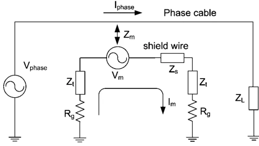
towers. ... 44 Figure 3.2 - Position of the sensor on the top of the tower. ... 45 Figure 3.3 - Genscape wireless monitoring system . ... 48 Figure 3.4 - Equivalent circuit for the induction of voltage on the shield wires: Iphase is the

current on the phase cable, Zm is the mutual impedance, Zt is the impedance of the

tower, Zs is the impedance of the shield wire, Rg is the tower grounding resistance,

Vm is the induced voltage, Im is the induced current, Vphase is the phase voltage,

and ZL is the load impedance. ... 49

Figure 3.5 - The equivalent circuit for the evaluation of the induced voltages and currents on the shiel wire and towers. ZT is the tower impedance plus the grounding

resistance, ZW is the wire impedance, Vm is the induced voltage, In is resulting

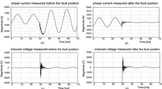
induced current. ... 50 Figure 3.6 - Line-to-ground fault currents before (a) and after (b) the short-circuit position;

Voltage induced on the shield wire before (c) and after (d) the short-circuit

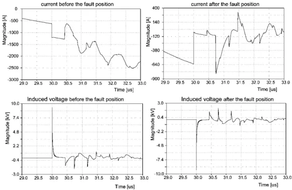
position. ... 51 Figure 3.7 - Details of the edges of the transient currents and the induced voltages of Figure

3.6. ... 52 Figure 3.8 - Currents in the shield wire and in the towers near the fault position, IS1 to IS7 are

the shield wire currents, IT1 to IT6 are the tower currents, Zf is the short-circuit

impedance, If is the short-circuit current (T1 to T6 are the identifications for tower

1 to tower 6). ... 53 Figure 3.9 - Waveforms of the transient currents in the shield wire and towers according to

Figure 3.8. ... 54 Figure 3.10 - Equivalent circuit for the high frequency induction in the shield wire, Zt e Zs

are the surge impedances of tower and shield wire, respectively, Rg is the tower grounding resistance, Vm is the induced voltage. ... 55

Figure 3.11 - Position of the sensor on the top of the tower (a), detail of the tip of the tower (b), and the detail of the coil (c). ... 56 Figure 4.1 - Block diagram of the wireless sensor. ... 60 Figure 4.2 -current induced by the fault. ... 61 Figure 4.3 - Overview of the wireless network communication of the detection and location

(23)

xiii

Figure 4.7 - Linear topology (a) and mesh topology (b) the dashed line circle around the source node indicates the range of the radio transceiver (equal for every node). . 68 Figure 4.8 - The alternative path at the end of the network ... 68 Figure 4.9 - MSC diagram of the data transmission process. ... 70 Figure 4.10 - Message types and fields. ... 71 Figure 4.11 - The SDL diagram of the flooding process. ... 73 Figure 4.12 - Message format with address fields. ... 74 Figure 4.13 - Allocation of 802.11 channels for 12 transmission lines, the numbers indicate

the channels. ... 75 Figure 4.14 - The path of the sync messages. ... 76 Figure 4.15 - The equivalent circuit of the shield wire and towers to evaluate the distribution

of currents: ZT is the tower and grounding impedance, ZER and ZEL are the

equivalent resistances to the right and to the left of the span, respectively, Vm and

In are the voltage and current induced. ... 80

Figure 4.16 - The current transformer and apparatus installed on shield wire, Im is the current

induced in the shield wire. ... 81 Figure 4.17 - The CT equivalent circuit, Rsec and Lm are the secondary resistance and

inductance of the CT, respectively, Im is the induced current and N is the number

of turns of the secondary of a window type CT. ... 81 Figure 4.18 - Power supply circuit. ... 82

Figure 4.19 - The output voltage of the power supply (a), the output of the PWM (b), and the current at the secondary of the current transformer (c). Vreg, Vop, and Isec refer to the labels in Figure 4.18. ... 84 Figure 5.1 - The stroke positions, span lengths and footing resistances used in the simulations. ... 86 Figure 5.2 - Simulated currents of a direct lightning stroke to the top of tower 4. ... 87 Figure 5.3 - Simulated currents of a direct lightning stroke to the middle of the span, between

towers 4 and 5. ... 87 Figure 5.4 - Simulated currents for a lightning stroke to phase cable, close to tower 4. ... 89 Figure 5.5 - The stroke points used in the simulations. ... 90 Figure 5.6 - Currents of a direct stroke to shield wire 1 in tower 3. ... 91 Figure 5.7 - Currents of a direct stroke to shield wire 1 at the middle of the span, between

(24)

xiv

Figure 5.11 - ATP saturable component: Lp, Rp, Ls and Rs are the primary inductance and resistance, and secondary inductance and resistance, respectively, Rmag is the magnetizing resistance, SATURA is the ATP support routine. ... 102 Figure 5.12 - The current induced in the 21th span and the CT output current. ... 102 Figure 5.13 - A piece of the diagram of the simulated overhead power line showing six spans

and the CT: the cables are modelled by the LCC objects, the grounded resistors represent the tower grounding resistances, RB is the burden resistor. ... 102

Figure 5.14 - Positions of the phase cables and shield wires, H varies for every tower

(dimensions in meters). ... 103 Figure 5.15 - Simulation scenario. ... 105 Figure 5.16 - The alternative paths of the network in a power line with branches. ... 114 Figure 5.17 - The simulation of branches. ... 115 Figure 5.18 - Communication in case of a failure of one sensor. ... 118 Figure 5.19 - The position of antennas in the field measurements. ... 119 Figure 5.20 - The tower as an obstacle inside the Fresnel zone. ... 120 Figure A 1 - Tower dimensions (m) and the positions of the phase cables (A, B, and C) and

the shield wire (S) (m). ... 135 Figure A 2 - The instant of the fault within the voltage cycle. ... 136

Figure B 1 - Tower dimensions (m) and the positions of the phase cables (A, B, and C) and the shield wire (S) (m). ... 137 Figure B 2 - The simulation diagram of a direct stroke to shield wire. ... 139 Figure B 3 – Shape of the lightning stroke current used in the simulations. ... 140 Figure C 1 - Tower dimensions (m) and the positions of the phase cables (A, B, and C) and

(25)

xv

List of Tables

Table 2.1 - The maximum difference between the top of towers as a function of the antenna elevation angle. ... 38 Table 4.1 - 802.15.4 and 802.11 transceivers. ... 77 Table 5.1 - Results for one set of simulations of a non-homogeneous power transmission line

(“Tn” is the abbreviation for “tower n”, “Tn-Tn+1” means between “tower n” and “tower n+1”). ... 88 Table 5.2 - Results for the simulations of a direct stroke to phase cable (shielding failure)

(“Tn” is the abbreviation for “tower n”). ... 89 Table 5.3 - Results for one set of simulations of a non-homogeneous power transmission line

(“Tn” is the abbreviation for “tower n”, “Tn-Tn+1” means between “tower n” and “tower n+1”). ... 92 Table 5.4 - Results for the simulations of a direct stroke to phase cable (shielding failure)

(“Tn” is the abbreviation for “tower n”, “Tn-Tn+1” means between “tower n” and “tower n+1”). ... 93 Table 5.5 - Lightning stroke position estimation using the values of Table 5.3 and Table 5.4

(“Tn” is the abbreviation for “tower n”). ... 95 Table 5.6 - Results of the fault simulations in T4. ... 97 Table 5.7 - Results of the fault simulations in the middle of the span (between T4 and T5). . 97 Table 5.8 -di/dt values for different types of transient disturbances. ... 99 Table 5.9 - Maximum power available simultaneously from eight spans. ... 101 Table 5.10 - Simulation results for the maximum power available simultaneously from ten

(26)

xvi

(27)

1

Chapter 1 Introduction

Accidental outages of electric power transmission lines have significant social and economic impacts in large areas, causing losses of various types. Each of these lines can carry power to several cities or even several states. Besides, large energy systems are interconnected and a problem with one transmission line can propagate to other lines causing problems in cascade. The outages are caused by short-circuits in the phase cables, disruptions of cables or lightning discharges that hit the power line directly.

1.1 The problem

Direct lightning strokes to power transmission lines are the main cause of faults [1]. Therefore, it constitutes a major problem for power distribution companies. It is of great relevance to determine if the cause of the power outage is a direct stroke or a short-circuit caused by other events like fire or trees. There is scientific and technological interest in low cost systems to identify, quickly and accurately, the incidence of direct strokes to the transmission line and locate the stroke point. Thus it will be possible to begin immediate corrective actions and effective preventive actions. Because the lines crosses great extensions of territory in regions that are often inhospitable, such a system allows a great reduction in the time wasted in the preventive or corrective actions.

1.2 The motivation

(28)

2

If the stroke location system has the additional feature of short-circuit fault location, the location system is more complete and useful. Besides, the usefulness is increased if the system can detect and locate short-circuit that do not cause a fault.

The known operational fault location systems perform the location through measurements at the ends of the transmission line and do not detect directly the lightning strokes to lines that caused an outage. There are few publications about direct stroke to power line location systems [2][3][4] and the existing operational systems combine a Fault Location System with a Lightning Location System (LLS) to perform the event correlation [5]. These systems do not detect the direct strokes nor the short-circuits that do not cause power outage.

1.3 The objectives

Events such as lightning and faults caused by fire and other phenomena can be monitored effectively and in real time by sensors distributed along the power transmission line, on the top of the towers, with communication via radio for transmitting data to a collection point. The sensors can be provided with local processing capacity that allows great flexibility in data collection, functioning as a network of "smart" sensors. The intelligent sensors can be equipped with a processor, memory, analog to digital converters, sensors and communication devices that allow making, storing and processing measurements, and running communication protocols, through which they can communicate more efficiently for data transmission. Technological developments and the spread of microcontrollers and wireless technologies made it feasible to create a low cost system for identification and location of direct strokes to transmission lines and short-circuit faults, by using intelligent sensors.

The goal of this work is to evaluate the feasibility of and to propose a system for detection and location of direct strokes and short-circuits (transient disturbances) in overhead power transmission lines (OPTL). In this work the whole system is studied and the main issues of the system are addressed:

a) How to detect the direct strokes and short-circuits with the sensors; b) How to locate the events;

(29)

3

1.4 The solution

The result of this work is a method to detect and locate direct lightning strokes and short-circuit faults in overhead power transmission lines using sensors on the top of the towers. The detection is performed by the measurement of induced currents in shield wires using wireless sensors that send these measurements to be processed by a computer at one of the ends of the transmission line. The wireless sensors are the nodes of a wireless network that transports the information to be processed. The transient disturbances are located by the computer after processing the information about the currents in the shield wires received from each sensor close to the disturbance. This work includes the analysis and the proposal of a low maintenance solution to supply power to the sensors without using photovoltaic (PV) cells and batteries, using the continuous power available in the shield wires.

1.5 The results

The method to detect and locate direct lightning strokes and the method to locate short-circuit faults was evaluated using simulations that showed their feasibility and accuracy. The operation of the wireless sensor network was simulated to verify the behavior of the high number of sensors operating in the peculiar linear topology. The field measurements showed the feasibility to use the well known wireless standards in the wireless network to guarantee a reliable operation. The simulations and field measurements showed the feasibility of using the power of the shield wires to feed the sensors eliminating the PV cells and batteries and their maintenance.

(30)

4

1.6 Text organization

(31)

5

Chapter 2 General Concepts

2.1 Transient disturbances

The power systems disturbances are mainly classified as steady-state and transient phenomena [6]. The transients induced by direct strokes to overhead power lines and the transients caused by short circuit faults are two important transient disturbances that can cause power outage with several consequences.

The direct lightning strokes to power transmission lines are the main cause of faults, representing about 65% of the events according to international statistics. In our state, Minas Gerais, Brazil, with high keraunic level, the faults in power transmission caused by lightning strokes represent 70% of events (20% being permanent), according to the state power company CEMIG (Companhia Energética de Minas Gerais) [1]. The direct strokes to phase cables can establish high overvoltages between phase conductor and earth. The overvoltage can cause the insulator failure and an electric arc between the conductor and the tower creating a short circuit path from phase conductor to ground [7]. The direct strokes to the shield wire of overhead power transmission lines produces high value of transient currents flowing in the shield wires and towers and corresponding high surge voltage on the top of the tower which can damage the insulators.

The short circuit faults can occur between one or more phases and ground, and between phases. Other causes of short-circuits are the fall of towers and the proximity of trees to cables. The calculations from CEMIG [8] show that the resistance of short circuits caused by strokes is low, between 0 and 10 . In case of short circuits caused by fire, the resistance is between 10 and 70 . In case of short circuits caused by threes, the resistance is above 70 .

2.2 Lightning strokes

(32)

6

most common are the cloud-to-cloud. Cloud-to-ground strokes are the most important due to the greater extent of the problems but represents less than 25% of the total. Approximately 90% of cloud-ground discharges are negative, i.e. the lower region of the cloud base is loaded negatively, inducing positive charges on the ground [9].

The phenomenon of atmospheric discharge consists of several steps. In case of negative cloud-to-ground type, first the cloud with the base charged with negative charges induces a positive charge in the ground establishing a great potential difference between its base and the ground (several megavolts). Under certain conditions, the electric field inside the base of the cloud reaches values above the dielectric strength of the air (3 MV/m). This condition creates an ionized channel of plasma with several tens of meters, know as stepped leader. This stepped leader moves toward the ground in straight segments with spacing of approximately 50 m in time intervals of the order of 1 µs [9]. When the stepped leader is close to the ground (hundreds of meters), there is the formation of an intense electric field between the front of the stepped leader and the ground with induction and consequent formation of positive discharges from the ground up, called upward leaders. With the meeting between the upward leaders and the stepped leader, there is the formation of the main discharge channel called return stroke with upside direction and possessing speed above 108 m/s, with average rise time of 10 µs and average duration of 100 µs [10]. The abrupt local expansion of the air due to intense channel discharge temperature causes the phenomenon called thunder.

In 80% of cases, after the first return stroke there are a series of subsequent return strokes. The first stroke and the unique stroke have similar characteristics. In case of subsequent strokes, they have different characteristics from the first stroke [11].

(33)

7

Figure 2.1 - Return stroke current measured at Morro do Cachimbo research station [13].

(34)

8

Figure 2.2 - Tower with shield wires.

2.3 Lightning location systems

(35)

9

Figure 2.3 - Lightning location system (LLS).

(36)

10

Figure 2.4 - Direction finder antenna, B is the magnetic flux generated by the lightning, is the angle between coil direction and the hit position.

The Time of Arrival system uses a different approach to locate the lightning stroke. The detection stations record the time of arrival of the electromagnetic field generated by the lightning. The differences between the time records of three or more stations are used to locate the hit position. There is a hyperbole associated to the difference of time between two stations which is the geometric place of hit positions that would result in the same time difference of arrival time between these two stations. The intersection of these hyperboles determines the hit position.

The location accuracy of these systems is of the order of several hundred meters [15].

2.4 Fault location systems

The fault locations systems usually perform the location of the fault using terminals installed at the ends of the transmission line to gather information from the phase cables. Two of the most used fault location systems are the impedance-based systems and the travelling wave systems [16]. The system can use one terminal at the end of the line, or two terminals, one at each end. The two terminal systems are more accurate than one terminal systems.

Two-terminal fault location techniques based on impedances usually use the following approach. The fault is at location m of the line from Bus G and (1–m) from Bus H (Figure

(37)

11

Figure 2.5 - Two terminal impedance-based fault location method [16].

VF is the voltage at the fault. The bus voltages and currents are as indicated in the figure.

Use of voltage/current relationships in all three phases (A, B, and C) yields the results shown in Equation (2.2) and Equation (2.2):

(VGF)abc = m ZLabc (IGF)abc + VF (2.1)

(VHF) abc = (1− m ) ZLabc ( IHF) abc + VF (2.2)

VF is the fault voltage on the fault resistance RF, VGF and VHF are the bus voltages in

fault condition, IGF and IHFare the line currents in fault condition, m is the distance to the fault

position, and ZLabc is the line impedance. Subtracting the two equations to eliminate the

unknown VFresults in Equation (2.3):

(VGF)abc − (VHF)abc = m ZLabc (IGF)abc + (m −1) ZLabc (IHF )abc (2.3)

This equation can be solved for the real m, and the phase values can be substituted with

the symmetrical components. The state power company CEMIG has a two terminal system with location accuracy of 2% of the line length that have located fault resistances up to 110 [8].

(38)

12

megahertz. These traveling waves have a front wave with fast rise time and a relatively slow fall time. The waves travel at speeds close to the light, from the point of failure toward the terminal points at buses A and B of the line as illustrated in Figure 2.6.

Figure 2.6 - Two terminal travelling waves fault location method.

A and B are the buses at the end of the power line with a length L and the fault occurs at

the distance x from bus A. ta and tb are the propagation time of the transient waves generated

by the fault to the buses A and B, respectively. The waves are not limited to the transmission

line where the fault occurred. They propagate through the adjacent electrical system with descending amplitude, as a result of the combined effects of line impedance and successive reflections. The fault location by traveling waves is based on the precise determination of the moment when the wave fronts pass through known points, usually substations located at the terminal points of the transmission line. Knowing the instant of time when the wave front arrives to terminals A and B of the transmission line (ta and tb) and starting from the length of

the line (L), it is possible to determine the location of the fault from the terminal (x) by the

formula:

2

) t (t c k L

x= + a − b (2.4)

where c is the speed of light (299.792.458 m/s) and k = 0.95 to 0.99 is a reduction factor

(39)

13

2.5 Modeling of transmission line towers and cables

The modeling of the power transmission lines is essential for the simulations performed in this work. To model a power line it is necessary to model the towers and the cables.

The towers are represented in the simulations by their surge impedance which has a critical role in the determination of the rise of potential at the top of the towers under lightning and transient fault conditions. Besides, the surge impedance of towers and cables determines the lightning and fault currents flowing through the towers. The rise of potential at the top of the towers can lead to back-flashover across the insulator strings.

Tower surge impedance determination includes both theoretical calculations and experimental measurements with models and full-scale towers. Experimental methods include the direct method [21] and the time-domain reflectometry method [22]. In the direct method the current is injected in the tower top and the ratio of the measured voltage and current records is calculated. In time-domain reflectometry method the tower impulse response of small-scale models is measured and analytical expressions are used for the calculation of the surge impedance based on traveling wave theory. Theoretical studies for predicting the surge characteristics of towers have been performed in the time domain by solving the electromagnetic field equations analytically [23][24][25]. The IEEE suggests a method to calculate the tower surge impedance [26], used in this work, based on the equation proposed by Chisholm et.al. [25]:

Z₀=60 ln cot 1

2tan

-1 Ravg

h₁+h₂ (2.5)

R_avg=r1h2+r2 h1+h2 +r3h1

h₁+h₂ (2.6)

where:

Z0=tower surge impedance

r1=tower top radius (m)

r2=tower midsection radius (m)

r3=tower base radius (m)

h1=height from base to midsection (m)

h2=height from midsection to top (m)

(40)

14

Z₀=60 ln 2 h2_r+r2 (2.7)

where Z0 is the tower surge impedance, h is the height of tower and r is the radius of the tower

base.

Modeling of cables is a well-known theme whose treatment is well defined in the literature. The Alternative Transient Program (ATP), used to perform the simulations of the power transmission lines [27] in this work, have line and cable support routines to simulate accurately the cables of a power transmission line. These routines are based on well-known and widely used theories well documented in [28] and simulate the cables for steady state 60 Hz analysis and for higher frequency transient analysis. There are several case studies showing that the simulation results using the ATP program and the line and cable support routines are close to the field measurements [28][29][30].

2.6 The Rogowski coil

The measurement of the transient currents can be carried out by a Rogowski coil which is a coil with turns equally distributed along a non magnetic core. The return wire goes back concentrically to avoid the external fields produced by external currents near the coil (Figure 2.7). The placement of the coil is very easy due to the construction of the coil in an open ring shape that is mechanically closed around the conductor of the current to be measured.

Figure 2.7 - Measurement of current using Rogowski coil, i(t) is the

current being measured, v(t) is the coil voltage, and K is a constant.

The Rogowski coil voltage (v(t)) is proportional to the rate of change of the current by

(41)

15 dt di A l N dt di K

v(t)= =− ₀ (2.8)

where µ0 is the vacuum permeability, N is the number of turns, l is the mean length of the

toroid and A is the area of the turn. Integrating the voltage v(t), we obtain an output voltage, vout(t), proportional to the original current i(t) by the time constant RC of the integrator:

Ai(t). l N RC 1 v(t)dt RC 1 (t)

v_out = = ₀ (2.9)

The most important characteristics of a Rogowski coil are large bandwidth, large range (from amperes to kiloamperes), good linearity (non-magnetic core), no saturation, easy installation, and galvanic isolation between the primary circuit and the measuring circuit [31]. The Rogowski coils are usually used to measure the stroke currents in the towers of lightning research stations [9].

2.7 The wireless networks

2.7.1 Network architecture overview

(42)

16

Figure 2.8 - The OSI model [32].

Figure 2.8 shows that the lower layers entities perform a node-to-node communication. The hosts in the Local Area Networks (LANs) and the routers in the LANs and in the Wide Area Networks (WAN) use the physical, link and network layers to communicate. Equipments like switches in the Local Area Networks (LAN) and wireless access points in the Wireless LANs use the physical and data link layers to communicate. The model shows that the communication between the upper layers (transport, session, presentation and application) is end-to-end (source and destination) [32].

(43)

17

The presentation layer provides independence from differences in data representation (e.g., encryption) by translating from application to network format, and vice versa. The presentation layer works to transform data into the form that the application layer can accept [32].

The session layer establishes, manages and terminates connections between applications. The session layer sets up, coordinates, and terminates conversations, exchanges, and dialogues between the applications at each end. It deals with session and connection coordination. Examples of session layer protocols are the Windows NetBIOS protocols [34].

The transport layer is responsible for error-free data delivery and in the proper sequence, flow control, multiplexing and error checking and recovery. Flow control manages data transmission between devices so that the transmitting device does not send more data than the receiving device can process. Multiplexing enables data from several applications to be transmitted onto a single physical link. Error checking involves the use of mechanisms for detecting transmission errors, while error recovery involves the action of requesting the retransmission of the data when errors occur [32]. The transport protocols used on the Internet are TCP (Transmission Control Protocol) and UDP (User Datagram Protocol). For certain applications the transport protocol may not be necessary. Some functions of this layer can be implemented in the application layer, or in the application. In this case, if a reliable service is necessary, the application has to implement error checking and recovery.

The network layer provides switching and routing technologies creating logical paths for transmitting data from node to node. Routing and forwarding are functions of this layer, as well as addressing, internetworking, error handling, congestion control and packet sequencing. The network protocol used on the Internet is the IP (Internet Protocol) protocol [32].

The data link layer provides reliable transit of data across a physical network link. In this layer, data packets are encoded and decoded into bits. It provides transmission protocol acknowledge and management and handles errors in the physical layer, flow control and frame synchronization [32].

(44)

18

single link of a network. LLC is defined in the IEEE 802.2 specification and supports both connectionless and connection-oriented services used by higher-layer entities. IEEE 802.2 defines a number of fields in data link layer frames that enable multiple higher-layer entities to share a single physical data link [35]. Besides, the LLC enables the upper layers to use different MAC layers, like the TCP/IP protocols in the wireless routers that use both the 802.3 Ethernet MAC [36] and 802.11 MAC [37]. The Media Access Control (MAC) sublayer of the data link layer manages upper layer access to the physical network medium. The IEEE MAC specification defines MAC addresses, which enable multiple devices to uniquely identify one another at the data link layer.

The standard of physical layer defines the electrical, mechanical, procedural, and functional specifications for activating, maintaining, and deactivating the physical link between communicating network systems. Physical layer specifications define characteristics such as voltage levels, timing of voltage changes, physical data rates, maximum transmission distances, and physical connectors. Physical layer implementations can be categorized as either LAN or WAN specifications. This layer conveys the bit stream (electrical impulse, light or radio signal) through the network at the electrical and mechanical level. Examples of LLC and MAC layers are the ones specified in IEEE 802.3 (Ethernet), IEEE 802.11b (Wireless LAN), and IEEE 802.15.4 (Wireless PAN) [38] standards.

The TCP/IP protocol suite has five layers (Figure 2.9). Usually, the application layer includes the functions of presentation and session layers, if necessary. Cryptography, a typical function of presentation layer, is partially implemented in the MAC layer of IEEE wireless standards.

Figure 2.9 - Internet communication layers.

(45)

19

these formats associated to the corresponding layer. The dashed line shows the real flow of the information data between the application layers of two equipments communicating in the network.

Figure 2.10 - The types of information formats and the flow of information between the layers.

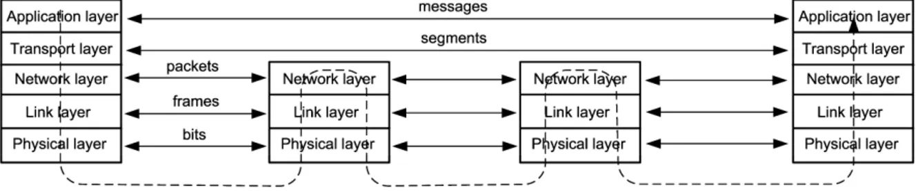
A message is the application layer PDU whose source and destination are application layer entities. A segment is the transport layer PDU whose source and destination are transport layer entities. A packet is the network layer PDU whose source and destination are network layer entities. A frame is the link layer PDU whose source and destination are data link layer entities. A PDU is composed of a header (and possibly a trailer) and upper-layer data. The header and trailer contain control information intended for the corresponding layer entity in the destination system. Data from the upper-layer entity is encapsulated between the header and trailer of the PDU. At the physical layer the information is transported by bits, the smallest logical unit of information in the network.

Data delivery services on the network can be divided into reliable services and unreliable services. In reliable services, there are mechanisms to ensure that the data sent by the source node will arrive without errors at the destination node. The source node is notified that the data was received, or that the network could not accomplish the delivery of data to the destination because of network problems. TCP transport layer of the Internet is an example of implementation of this type of service. These mechanisms are not implemented in the unreliable services. The source node sends the data and there is no guarantee of delivery of the data to the destination. The UDP protocol of the Internet is an example of implementation of this type of service.

(46)

20

Connection-oriented service has three phases: connection establishment, data transfer, and connection termination. During connection establishment, the end nodes may reserve resources for the connection. The end nodes also may negotiate and establish certain criteria for the transfer, such as a window size used in the connections. The data transfer phase occurs when the data is transmitted over the connection. During data transfer, most connection-oriented services will monitor for lost packets and resend them. The layer that implements the service is generally also responsible for ordering the packets in the right sequence before passing the data to the upper layer in the communication stack. When the transfer of data is complete, the end nodes terminate the connection and release resources reserved for the connection.

In general, connection-oriented services provide some level of delivery guarantee, whereas connectionless services do not, therefore the connection oriented protocols are used to implement a reliable service. The connectionless protocols are usually used to implement an unreliable service but it is possible to have a connectionless reliable service, known as confirmed datagram. Connection-oriented network services have more overhead than connectionless ones.

An example of connection oriented protocol in the transport layer is the TCP protocol. An example of connectionless protocol in the transport layer is the UDP protocol. The connection oriented protocols are implemented in the upper layers (from transport to application layers) while the connectionless protocols can be implemented in every layer. An example of connectionless network protocol is the IP protocol of Internet. The connectionless protocol data unit is known as datagram. IP uses datagram packets and UDP uses datagram segments.

(47)

21

2.7.2 IEEE wireless standards

The Institute of Electrical and Electronics Engineers (IEEE) has produced the series of standards 802.X, which encompassed the wired Local Area Network (LAN), the Wireless LAN (WLAN), Wireless Metropolitan Area Network (WMAN), and Wireless Personal Area Network (PAN). The scope of IEEE 802 is the two lower network layers, the physical and the link layers. The wireless network standards supported by the industry are 802.11 (WLAN), 802.15 (WPAN) and 802.16 (WMAN). These standards specify the physical layer and the MAC layer services defining how each network node communicates with other node exchanging frames. The IEEE 802.2 link layer control (LLC) [35], is used with these MAC layers as an interface with the upper layers like the IP and the TCP/UDP Internet layers.

IEEE 802.16 [39], known as WiMax because of the alliance formed to certify the 802.16 products, is a specification for fixed broadband wireless metropolitan access networks (WMANs). It is a long-range technology which can reach up to 50 km in line-of-sight at data rates up to 70 Mbps.

The 802.15 standard defines three specifications for WPAN: the 802.15.1 for the Bluetooth technology [40]; the 802.15.3 for high rate WPAN [41]; and the 802.15.4 for low rate WPAN [38]. The 802.15.1 is best suited for connecting PDAs, cell phones and PCs in short intervals. The 802.15.3 standard has a high bandwidth up to 55 Mbps and low transmission range, like Bluetooth, and is suite for short-range multimedia streaming. The 802.15.4 is the standard of choice to be used on most Wireless Sensor Networks (WSNs). The physical layer technologies used in 802.15.4 has good performance against noise and interferences. The transmission range is high, of the order of kilometers as we show later, especially in the 868/915 MHz bands.

(48)

22

smartphones over a wide area. Like 802.15.4, 802.11 have good performance against noise and interferences because of the use of similar technologies in the physical layer.

The wired and the wireless networks can use the same transport and network layers, usually TCP/UDP and IP, respectively, and the same 802.2 LLC sublayer. Only the MAC sublayer and physical layer are different at each wired or wireless technology (Figure 2.11) [35].

Figure 2.11 - Stack of IEEE 802.x standards [35].

Figure 2.12 shows the IEEE 802.x standards. There are three possible physical layers technologies for 802.11: Frequency Hopping (FH), Direct Sequence Spread Spectrum (DSSS) and infrared light. There is only one physical layer technology used in 802.15.4, the DSSS. DSSS is a transmission technique that has good performance against noise and interferences. The communication at physical layer of these wireless standards is half-duplex. Each network node transmits or receives, not both at the same time.

Figure 2.12 - 802.11 and 802.15.4 services.

(49)

23

the application layer [42]. In the ZigBee specification there is no transport layer. ZigBee was primarily designed for the wide ranging automation applications and to replace the existing non-standard technologies. Figure 2.13 shows the ZigBee layers [8].

Figure 2.13 - ZigBee layers [8].

(50)

24

Figure 2.14 - Basic access mechanism [37].

For a single node do not monopolize the channel, it starts the counter whenever two or more packages were transmitted. The nodes have no way to detect whether there was a collision or not because they are unable to transmit and listen to the channel simultaneously [43]. Then, an Acknowledge Frame (ACK) is sent by the destination node immediately after a short period of time called Short Interframe Space (SIFS) whenever a packet is received without error. If an ACK is not received after a pre-defined period of time, there was a collision or a loss of packet and the source node reschedules the transmission according to the size of the window of backoff.

(51)

25

Figure 2.15 - The problem of the hidden terminal (B) [43].

(52)

26

Figure 2.16 - RTS/CTS mechanism [37].

The radio frequencies allowed for use in wireless networks are the frequencies of ISM (Industrial, Scientific and Medical) bands, defined by ITU-R (International Telecommunication Union - Radio Communication Sector), which do not require special licensing for operation. The ranges 433.05–434.79 MHz, 902–928 MHz, 2.4–2.5 GHz, and 5.725–5.875 GHz are the most used. Lower frequencies allow higher transmission range, because they are less attenuated, but are more susceptible to fading (unwanted reflections on obstacles) that degrades the signals. As the sensors will operate in open environments, without buildings nearby, the problems of fading are small. IEEE 802.11 uses the ranges 2.4– 2.5 GHz, and 5.725–5.875. The IEEE 802.15.4 uses the ranges 902-928 MHz and 2.4-2.5 GHz. The IEEE 802.11 standard has amendments to specify additional functionalities such as data rates, frequency of operation and data encoding. The most used are the amendments “a”, “b”, and “g”. The basic IEEE 802.11 and the amendments “b” and “g” operate in the 2.4 GHz band. IEEE 802.11a operates in the 5 GHz band. The basic IEEE 802.11 operates with the data rates 1 Mbps and 2 Mbps. IEEE 802.11a operates with data rates between 6 and 54 Mbps [44]. IEEE 802.11b data rates between 1 Mbps and 11 Mbps [45]. IEEE 802.11g operates with data rates between 1 Mbps and 54 Mbps [46].

(53)

27

MHz (with the exception of channel 14) (Figure 2.17) [45]. To use non overlapping channels, only the channels 1, 5, 9 and 13 can be used.

Figure 2.17 - 802.11 channels [47].

For 802.15.4, the spectrum is divided into 10 channels in 915 MHz band and 16 channels in the 2.4 GHz band (Figure 2.18) [38]. The center frequency of each channel is separated by 5 MHz (with the exception of channel 14) in the 2.4 GHz band and separated by 2 MHz in the 915 MHz band.

Figure 2.18 - 802.15.4 channels [48].

2.7.3 Network topologies

(54)

28

Figure 2.19 - Network topologies.

a) Bus Topology

In this topology the nodes are connected to a single common backbone. This common medium is a shared communication path for the nodes. Each node communicates directly to other node or to every node simultaneously. The shared media can be a cable like the old Ethernet 10Base2 or 10Base5, or a radio channel, like the 802.11 wireless networks.

b) Ring Topology

In this topology each node can communicate with up to two neighbors. The message travels through the ring in either clockwise or anti-clockwise direction. The FDDI and Token ring networks are examples of ring topology.

c) Star Topology

This network topology centralizes the communication in a central node responsible to forward the data to the destination node. An example of this topology is the common Ethernet network with fast Ethernet switches or hubs.

d) Tree Topology

(55)

29

e) Mesh Topology

In this topology every node can be connect to one or more neighbor nodes without any specific structure. Each node has to operate as a router to forward the data to the destination through its neighbors. The data passed on to the network can take several paths to reach the destinations, unlike the other topologies. If every device is connected to every other device the network is called full mesh.

f) Linear topology

In the linear topology the nodes are arranged in line and every node communicates with a neighbor behind and a neighbor ahead. When the nodes are geographically arranged in line (physical linear topology), but the logical topology is mesh, the topology is called nearly linear topology. Figure 2.20 shows an example of nearly linear topology and the equivalent mesh topology. For the sake of simplicity, the nearly linear topology will be referred as linear topology in this work.

Figure 2.20 - Nearly linear topology and the equivalent mesh topology.

2.7.4 Types of wireless Networks

(56)

30

Figure 2.21 - Infra-structured wireless network.

The second type of network is a wireless network without infrastructure, commonly known as Ad Hoc network. They have no fixed routers. All nodes can be connected in an arbitrary manner. These nodes function as routers, which discover and maintain routes to other nodes in the network. The mobile wireless network used on military vehicles to change information in the battlefield is an example of Ad hoc network. In this context, every sensor is a node with routing capacity. Figure 2.22 shows an Ad hoc network of notebooks.

Figure 2.22 - Infra-structured wireless network.

2.7.5 Ad hoc routing protocols

(57)

31

Table-driven routing protocols attempt to maintain consistent, up-to-date routing information from each node to every other node in the network. Each node must maintain one or more tables to store routing information. The changes in network topology trigger the propagation of updates throughout the network in order to maintain a consistent network routing information.

The source-initiated on-demand routing protocols employ a different approach from table-driven routing. This type of routing protocol creates routes only when triggered by the source node. When a node requires a route to a destination, it initiates a route discovery process within the network. This process is completed once a route is found or all possible route paths have been examined. Once a route has been established, it is maintained until either the destination becomes inaccessible along every path from the source or until the route is no longer desired.

There are several protocols of each type [50]. Figure 2.23 shows a list of the most known Ad Hoc protocols and the classification of each one: Destination-Sequence Distance Vector (DSDV), Optimized Link State Routing (OLSR), ZigBee Routing, Ad hoc On Demand Distance Vector (AODV), Dynamic Source Routing protocol (DSR), Dynamic MANET On-demand (DYMO) and Temporally-Ordered Routing Algorithm (TORA). ZigBee Routing is considered to be a hybrid protocol because it uses two routing protocols: Hierarchical Tree Routing (HTR) which is a table driven protocol and modified AODV which is an on-demand protocol. HTR is used for nodes without routing capability and AODV is used for router nodes.

Figure 2.23 - Some common Ad Hoc routing protocols.

(58)

32

(HWMP), combines the concurrent operation of a proactive tree-oriented approach with an on-demand distributed path selection protocol derived from the AODV. Nevertheless, the working group has not finished their work and the HWMP is not concluded. On the other hand, the Zigbee standard defined the ZRP that uses HTR and modified AODV. The AODV of ZigBee specification has modifications to minimize the overhead [52].

2.7.6 The AODV protocol operation

(59)

33

Figure 2.24 - The operation of the AODV protocol [50].

2.7.7 Wireless Sensor Netwoks

A wireless sensor node consists of components for sensing, computing, communication, actuation, and power supplying. These components are integrated on a single or multiple boards, and packaged in a small case. With state-of-the-art, low-power circuit and networking technologies, a sensor node powered by AA batteries can last for years with a low duty cycle working mode. A WSN usually consists of tens to thousands of such nodes that communicate through wireless channels for information sharing and cooperative processing. WSNs can be deployed on a large geographical scale for environmental monitoring and habitat study, over a battle field for military surveillance and reconnaissance, in emergent environments for search and rescue, in factories for condition based maintenance, in buildings for infrastructure health monitoring, and many other applications.

(60)

34

working modes. Location and positioning information can also be obtained through the Global Positioning System (GPS) or local positioning algorithms. All this information can be gathered from the sensors across the network and processed to construct a global view of the monitoring phenomena. The basic concept behind WSNs is that, despite the limitations in the capability of each individual sensor node, the aggregate power of the entire network is sufficient for the required work. This is a fundamental difference between the WSNs and the traditional wireless networks like the Wi-Fi installations in the offices, campi and public places. While the wireless technology is basically the same, the sensor nodes in the WSNs work to reach a common objective of the system, while in the traditional wireless networks the individual station nodes work to accomplish the individual objective of each user. In the context of power transmission lines, the sensor nodes have a common objective: to gather information from the line to allow the system to detect, identify and locate direct lightning strokes to the line or short-circuits in the phase cables.

2.8 Transmission range of radio

The transmission range of wireless equipments is an important issue in the network operation. The continuous and reliable operation of these equipments depends on the signal received from the neighbors. The open field operation of wireless sensors and other wireless equipments can be analyzed theoretically estimating the attenuation of the signal in line-of-sight operation.

2.8.1 Radio attenuation in free space

The power received by the wireless sensor in free space without obstacles, can be calculated by the Friis formula [53]:

( )

2 2

2 r t t r d 4 G G P (d)

P = (2.10)

where Pr is the power at the reception, Pt is the transmit power, Gt and Gr are the gains of

transmitter and receiver antennas, respectively, d is the distance between the antennas and is

the wavelength. With this formula, the range (d) can be calculated using the receiver

sensibility as the value of the power received:

log (d) =

20 1 _[Pt

(61)

35

where f is the frequency in MHz, dBm means that the parameter is in dB milliwatts, and dBi

means that the gain is in dB relative to an isotropic antenna. Including a gain margin (M) in

dB the value of range can be calculated by the equation below:

log (d) =

20 1 _{. [Pt}

dBm - PrdBm + GtdBi + GrdBi - 20.log(f) + 27.54 + MdB] (2.12)

The Friis formula is accurate at unobstructed Line of Sight (LOS) path at low distances. Above a critical distance, the two path model (two-ray ground reflection model) [54] is more accurate and includes a ground reflection path besides the direct path of Friis model:

4 2 r 2 t r t t r d h h G G P (d)

P = (2.13)

where hr and ht are the height of transmitter and receiver antennas (meters), respectively. The

critical distance (dc) in meters is:

λ π _r _t

c 4 h h

d = (2.14)

If the distance between the antennas is less than dc, the Friis model must be used

otherwise the two path model must be used.

To have a propagation of the signal in conditions close to the free space, the volume of the Fresnel ellipsoid (Figure 2.25) [55] between the transmitter and receiver must be free of obstructions.

Figure 2.25 - The first Fresnel zone.

(62)

36

(

₁ ₂

)

2 1 1 d d f d d c F + = (2.15)

where c is the speed of light (m/s), d1 is the distance (m) from transmitter to the obstacle, d2 is

the distance from obstacle to the receiver, and f is the frequency (Hz).

The radius of the first Fresnel zone (F1) (m) in the middle of the path is:

f 4

d c

F₁= (2.16)

If 60% or more of first Fresnel zone have no obstruction, we have the conditions close to the free space. If h is the length of the obstacle that enters the volume of the ellipsoid, the

obstruction is calculated by h/F1. For h/F1=0.5 the attenuation is 3 dB and for h/F1=1 the

attenuation is -40 dB for flat earth surface [55], as usually is the case for the sensors operating on OPTLs.

2.8.2 Weather attenuation

The system must operate on any weather conditions. Therefore, it is necessary to evaluate the additional attenuation of the signal caused by rain and snow. The rain attenuation (Ar), in dB/km, can be estimated by the following formula [56]:

Ar = K R (2.17)

where K and are constants that depend on the frequency, and R is the rate of rain in mm/hr.

For a heavy rain with the high rate of 250 mm/hr of water, the attenuation at 2.4 GHz is less than 0.1 dB/km. At 5.15 GHz the attenuation is 1.5 dB/km.

The snow attenuation (As) can be estimated by the following formula [57]:

λ λ R 00224 . 0 00349 . 0

A_s = R1₄.6 + (2.18)

where is wave length (m) and R is the water equivalent of snow rate (mm/hr). For a heavy

snow with the high rate of 50 mm/hr of equivalent water, the attenuation at 2.4 GHz is only 0.009 dB/km and at 5.15 GHz is 0.02 dB/km.

(63)

37

2.8.3 The role of antennas in the transmission range

The antenna is very important to determine the maximum range of the radio transceiver because the gain significantly affects the range of the sensor. The antenna gain is a function of its directionality. An isotropic antenna irradiates the power equally in all directions. The free space models described above consider this type of irradiation in their formulas and include the antenna gain to account for the mode of irradiation of real antennas that do not irradiate in all directions. They concentrate the power in the horizontal (azimuth) and/or vertical (elevation) plan. The higher is the directionality, the higher is the gain of the antenna.

Special attention must be paid to the installation of the sensors. Because of the high number of sensors, the installation procedure must be simple. Therefore, antennas with directionality in both the horizontal and vertical plane must be avoided because it would be necessary to align the antennas to optimize the range. The transmission lines also can change direction at angles up to 90 degrees because of the topography of the terrain. The lines may also have branches in which case a sensor has to communicate with other sensors that are not positioned in line. The choice should be for the omnidirecional antennas in the horizontal plane so that the technicians have to concern only to install the antenna in a vertical position.

The vertical plane must have an elevation angle so that the irregularities of the terrain (hills and valleys) do not affect significantly the range of the transceivers (Figure 2.26).

Figure 2.26 - The elevation angle of the antenna and the difference in the tower levels.

In Figure 2.26 the angle E must be at most half the elevation angle of the antenna. To keep the neighbor sensor inside the elevation angle of the antenna, the minimum value of elevation angle of the antenna ( ) can be calculated as a function of the distance between the towers (D) and the difference of the heights of the towers (H):

Detecção e localização de distúrbios transitórios em linhas de transmissão de energia utilizando sensores sem fio

Universidade Federal de Minas Gerais

Escola de Engenharia

Programa de Pós-Graduação em Engenharia Elétrica

Detecção e Localização de Distúrbios Transitórios

em Linhas de Transmissão de Energia Utilizando

Sensores sem Fio

Dênio Teixeira Silva

Orientador: Prof. Dr. Julio Cezar David de Melo (UFMG)

Co-Orientador: Prof. Dr. José Luiz Silvino (UFMG)

Universidade Federal de Minas Gerais

Escola de Engenharia

Programa de Pós-Graduação em Engenharia Elétrica

Detection and Location of Transient Disturbances

in Power Transmission Lines Using Wireless

Sensors

Dênio Teixeira Silva

Advisor: Prof. Dr. Julio Cezar David de Melo (UFMG)

Co-Advisor: Prof. Dr. José Luiz Silvino (UFMG)

Agradecimentos

Resumo

Abstract

Contents

Abbreviations

List of Figures

List of Tables

Chapter 1

Introduction

1.1 The problem

1.2 The motivation

1.3 The objectives

1.4 The solution

1.5 The results

1.6 Text organization

Chapter 2

General Concepts

2.1 Transient disturbances

2.2 Lightning strokes

2.3 Lightning location systems

2.4 Fault location systems

2.5 Modeling of transmission line towers and cables

2.6 The Rogowski coil

2.7 The wireless networks

2.7.1 Network architecture overview

2.7.2 IEEE wireless standards

2.7.3 Network topologies

2.7.4 Types of wireless Networks

2.7.5 Ad hoc routing protocols

2.7.6 The AODV protocol operation

2.7.7 Wireless Sensor Netwoks

2.8 Transmission range of radio

2.8.1 Radio attenuation in free space

( )

(

)

2.8.2 Weather attenuation

2.8.3 The role of antennas in the transmission range