Effects of Geopotential and Atmospheric Drag Effects on Frozen Orbits Using Nonsingular Variables

(1)

Research Article

Effects of Geopotential and Atmospheric Drag Effects on

Frozen Orbits Using Nonsingular Variables

Paula Cristiane Pinto Mesquita Pardal,

1

Rodolpho Vilhena de Moraes,

2

and Helio Koiti Kuga

3

1_{Engineering School of Lorena (EEL/USP)-LOB, Estrada Municipal do Campinho, s/n, 12602-810 Lorena, SP, Brazil} 2_{São Paulo Federal University (UNIFESP)-ICT, Rua Talim, 330 Vila Nair, 12231-280 São José dos Campos, SP, Brazil} 3_{National Institute for Space Research (INPE)-DMC, Avenida dos Astronautas, 1758 Jardim Granja,}

12227-010 S˜ao Jos´e dos Campos, SP, Brazil

Correspondence should be addressed to Paula Cristiane Pinto Mesquita Pardal; [email protected]

Received 13 April 2014; Accepted 17 June 2014; Published 3 July 2014

Academic Editor: Silvia Maria Giuliatti Winter

Copyright © 2014 Paula Cristiane Pinto Mesquita Pardal et al. his is an open access article distributed under the Creative Commons Attribution License, which permits unrestricted use, distribution, and reproduction in any medium, provided the original work is properly cited.

he concept of frozen orbit has been applied in space missions mainly for orbital tracking and control purposes. his type of orbit is important for orbit design because it is characterized by keeping the argument of perigee and eccentricity constant on average, so that, for a given latitude, the satellite always passes at the same altitude, beneiting the users through this regularity. Here, the system of nonlinear diferential equations describing the motion is studied, and the efects of geopotential and atmospheric drag perturbations on frozen orbits are taken into account. Explicit analytical expressions for secular and long period perturbations terms are obtained for the eccentricity and the argument of perigee. he classical equations of Brouwer and Brouwer and Hori theories are used. Nonsingular variables approach is used, which allows obtaining more precise previsions for CBERS (China Brazil Earth Resources Satellite) satellites family and similar satellites (SPOT, Landsat, ERS, and IRS) orbital evolution.

1. Introduction

he orbital motion of an the artiicial satellite free of dis-turbing efects, named Keplerian motion, would be ellipses with constant sizes and eccentricities, in permanent planes, where the satellites would stay indeinitely. Some of the major perturbations that afect the orbital elements of an artiicial Earth satellite are as follows: nonhomogeneity of Earth’s mass distribution, sun-moon gravitational attraction, solar radiation pressure (direct and albedo), atmospheric drag, forces due to Earth’s tides, Poynting-Robertson drag, and Yarkovsky efect.

For orbital control purposes, it can be important that some orbital elements stay frozen, that is, with near constant values, in order to facilitate some maneuvers adjustment. Especially for maneuvers that have been carried out at INPE (National Institute for Space Research) Satellite Tracking and

Control Center (TSCC), with CBERS family, it is important that eccentricity and argument of perigee stay frozen.

he notion of frozen orbits goes back to many years, the history of which is well explained in [1, 2]. Due to their scientiic interest, frozen orbits concept has been also investigated around planetary satellites and asteroids [3,4]. Many investigators have contributed research; in order to predict the long-term evolution of the eccentricity and argu-ment of perigee without numerical integration, an analytical method based on the Delaunay variables was employed in [5]; and a simple solution has been developed for the long-term behavior of a near-circular orbit in a zonal gravity ield in [6], linearizing the singly averaged variational equations of motion and eliminating a degree of freedom with an integral of motion. he constraint equation for Earth frozen orbits, based on the Lagrange’s planetary equations, can be obtained for the gravity model involving higher degree zonals in [2].

(2)

Basically, the odd terms of geopotential, responsible for the long period efects, give rise to the frozen orbits. he inluence of geopotential perturbations on frozen orbits has been studied by several authors, including Cutting et al. [7], where secular and long period terms of geopotential up to�₃ are considered.

In the present work, such study is extended in order to verify the inluence of perturbations due to geopotential up to

�5terms and atmospheric drag on frozen orbits. Nonsingular

variables [8] are also introduced, turning analytical formulas suitable for very low eccentricity orbits application. Brouwer theory [9] is used to express analytically secular and long period terms due to geopotential for eccentricity and argu-ment of perigee. he inluence of atmospheric drag is also analytically expressed, using Brouwer and Hori theory [10].

In artiicial satellite theory, several analytical models have been proposed to describe the atmospheric density [11]. However, in general, the more realistic are the models, the more diicult is the solution of the motion equations. Both Brouwer and Brouwer and Hori theories are convenient for analytical developments and furnish reasonable orders of magnitude accuracy.

hese analytical expressions enable carrying out the temporal behavior analysis of eccentricity and argument of perigee in the neighborhood of a frozen orbit, as well as calculating the magnitude of the perturbations due to geopotential and atmospheric drag.

Such development will allow more precise predictions for the orbital maintenance and evolution of CBERS family and similar satellites.

2. Frozen Orbits Concept

A frozen orbit is characterized by keeping (or trying to keep) the argument of perigee and the eccentricity of an orbit constant, so that, for a given latitude, the satellite always passes at the same altitude, beneiting the users through this regularity. In another way, this type of orbit maintains almost constant altitude over any point on Earth surface. he design of frozen orbits involves selecting the correct values of eccentricity and argument of perigee, for a given semimajor axis and orbital inclination (in which critical value of 63.43∘ is an intrinsic singularity in the artiicial satellite theory [12]). he analytical nonlinear system of equations considering geopotential perturbations up to�₃terms are as follows [7]:

��

�� = 3��2� 2 �

�2_{(1 − �}2₎2(1 − 54sin 2_�)

× {1 + �3�� 2�2� (1 − �2)(

sin2� − �2cos2�

�sin� )sin�} = 0,

��

�� = 3��3� 3 �sin�

2�3_{(1 − �}2₎2(1 − 54sin

2_�)_cos_{� = 0,}

(1) wherea,e,i, and�are the classical orbital elements: semi major axis, eccentricity, inclination, and argument of perigee,

respectively;�_� is the Earth equatorial radius;� = √�/�3 is the satellite mean motion; � is the Earth gravitational constant; and �₂ and �₃ are the second and third gravity coeicients, respectively.

Equation (1) shows that perturbations efects in the eccentricity vanish for values of�equal to 90∘and 270∘.

3. Secular Perturbations and Long Period

Terms Using Nonsingular Variables

Brouwer [9] and Brouwer and Hori [10] analytical develop-ments allow analyzing the efects of the perturbations due to geopotential up to�₅order and to atmospheric drag on the neighborhood of a frozen orbit. Such equations are expressed in terms of the Keplerian orbital elements and are related to the disturbances on eccentricity and argument of perigee. However, these equations are placed so that singularity points may occur. Especially for the eccentricity values used by INPE, which applies frozen orbits theory on CBERS family, it indeed occurs [13,14].

With a view to eliminate the singularity points, a variables change is needed. Brouwer and Brouwer and Hori analyt-ical equations were rewritten using nonsingular variables approach. As consequence, eccentricity and argument of perigee no longer explicitly appear in the rewritten equations. he nonsingular variables,�and�, used by INPE TSCC and deined in terms of the eccentricity and the argument of perigee, are as follows [8]:

� = �cos�, � = −�sin�. (2)

Consequently, the eccentricity and the argument of perigee are given by

� = √�2_{+ �}2_, _{� =}_arctan

(−��). (3)

In order to carry out the variables change for eliminating the singularity points, other trigonometric expressions were rewritten in terms of nonsingular variables:

sin� = �

√�2_{+ �}2, cos� = � √�2_{+ �}2,

sin(2�) = 2��

√�2_{+ �}2, cos(2�) = � 2_{− �}2

√�2_{+ �}2.

(4)

he analytical equations for the frozen orbits dynamics,

(3)

0.0000 0.0004 0.0008 0.0012 0.0016 0.0020 0.0024

0

Eccen

trici

ty

Argument of perigee (deg) Perturbations due to geopotential up toJ3

40 80 120 160 200 240

0

Argument of perigee (deg)

40 80 120 160 200 24

�0= 90 ∘

�0= 100

∘

�0= 110

∘

�0= 120

∘

�0= 130

∘

(a)

0.0000 0.0004 0.0008 0.0012 0.0016 0.0020 0.0024

Eccen

tr

ici

ty

Perturbations due to geopotential up toJ3and atmospheric drag

0 40 80 120 160 200 240

�0= 90

∘

�0= 100

∘

�0= 110

∘

�0= 120

∘

�0= 130

∘

(b)

Figure 1: Phase plane diagram considering perturbations due to geopotential up to�₃and due to�₃and atmospheric drag for 300 days.

using nonsingular variables approach are presented in the Appendix, since the formula are too large to be displayed explicitly in the text.

4. Results and Analysis

he solutions for ̇� and ̇� equations, which are explicitly written in the Appendix, were obtained using CBERS-1 satellite real orbital data. Perturbations due to geopotential up to �₅ and atmospheric drag were analytically included and rewritten in terms of nonsingular variables. Results were plotted using a phase plane of eccentricity and argument of perigee, which is analogous to the system state evolving over time. Here, the period of time corresponds to 300 days. Such results allowed evaluating frozen orbits behavior.

In this application, the orbit was considered frozen when the argument of perigee was�= 90∘. he graphics aterwards show that the orbit starts escaping from its initial position if the arguments of perigee values are much diferent from 90∘ and that it is inclined to be conined and cycle-limited when such values are closer to 90∘.

First, a dynamic model including perturbations due to geopotential up to�₃only was considered. In a second step, the model took into account the efects due to geopotential up to �₅. Finally, a model including perturbations due to geopotential up to �₅ terms and atmospheric drag was analyzed. he drag efects analysis occurred for two diferent geopotential model accuracy levels: up to�₃terms only and up to�₅terms.

With the dynamical model development (i.e., a model consisting of more disturbing efects), a greater accuracy was expected for the frozen elements. First of all, a greater prevision capacity of these elements variations was expected, when compared to the results including terms up to�₃only.

In fact, the amplitudes of variation of argument of the perigee and eccentricity decreased when geopotential terms up�₅and atmospheric drag efects were included, as it will be shown next.

he results were obtained for the following CBERS-1 initial orbital elements:

(i) semimajor axis (�₀): 7148.763 km, (ii) eccentricity (�₀): 0.0011934, (iii) orbital inclination (�₀): 98.4896∘,

(iv) argument of perigee (�₀): from 90∘ up to 130∘ (step 10∘).

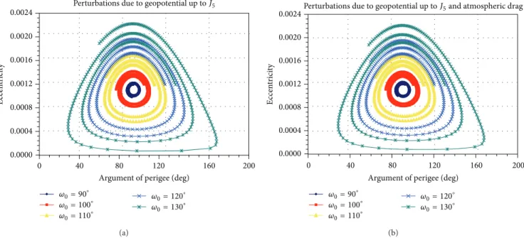
Figures 1and 2show curves obtained for ive diferent initial conditions. Such graphics were based on the solution of (2) and (4), both rewritten in nonsingular variables.Figure 1

shows the results for two models: geopotential up to�₃only and geopotential up to�₃included in atmospheric drag. In

Figure 2, the results for other two models are presented:

geopotential up to�₅and a more complete dynamic model that takes into account geopotential up to�₅and atmospheric drag. Regarding the atmospheric drag, the solar lux used was F10.7 of 250, which denotes the maximum solar activity and manifests itself on augmented atmospheric densities and, consequently, on higher atmospheric drag efects.

From Figures 1 and 2, it is noticeable that the curves

ofFigure 2 have less amplitude of variation for the frozen

elements than the irst one. Besides, if the two graphics of

Figure 1are compared amongst themselves, the inclusion of

(4)

0.0000 0.0004 0.0008 0.0012 0.0016 0.0020 0.0024

Eccen

tr

ici

ty

0 40 80 120 160 200

Perturbations due to geopotential up toJ5

�0= 90

∘

�0= 100

∘

�0= 110

∘

�0= 120

∘

�0= 130

∘

(a)

0.0000 0.0004 0.0008 0.0012 0.0016 0.0020 0.0024

Eccen

tr

ici

ty

Perturbations due to geopotential up toJ5and atmospheric drag

0 40 80 120 160 200

�0= 90

∘

�0= 100

∘

�0= 110

∘

�0= 120

∘

�0= 130

∘

(b)

Figure 2: Phase plane diagram considering perturbations due to geopotential up to�₅and due to�₅and atmospheric drag for 300 days.

Table 1 shows the maximum amplitudes of variation of

eccentricity and argument of perigee,Δ� and Δ�, for ive initial conditions. From Table 1, it is possible to observe that the magnitudes decrease when the perturbations due to geopotential up to�₅and atmospheric drag are included in the dynamic model, although the greater decreases occur with the inclusion of perturbations due to geopotential up to

�5.

FromTable 1, the amplitude of variation of the argument

of perigee decreases when geopotential terms up to�₅ and atmospheric drag terms are included. his behavior happens again for all initial conditions. If the argument of perigee initial values are far from the frozen orbits conditions (�= 90∘), the cycles including�₅ and atmospheric drag are still complete, while the cycles including�₃only start demeaning, as can be seen inFigure 1. In other words, the inclusion of the efects due to geopotential up to�₅and atmospheric drag improves the prevision precision of the argument of perigee. With respect to the eccentricity, the reduction is subtler, but it still occurs, since one of the atmospheric drag efects is to circularize the orbit (because the drag acts reducing the semimajor axis of the orbit).

In practice, the theory using only terms factored up to�₃ can persuade to wrong needs of orbital maneuver corrections. If it is supposed, for instance, that the mission requires a perigee value between 90∘±10∘, the�₃dynamic model would foresee a corrective maneuver, while the model including�₅ and atmospheric drag excludes the need of a maneuver, as can be seen on the irst line ofTable 1. So, the conclusion is that it is imperative for the inclusion of geopotential terms up to

�5and atmospheric drag terms to improve the precision on

planning of maneuvers carried out by INPE TSCC.

As shown inFigure 2andTable 1, the more meaningful decreases on the frozen elements amplitudes of variation occurred when the geopotential was factored up to�₅. his

way,Figure 3isolates the geopotential up to�₃and up to�₅

efects from the atmospheric drag ones, and only results due to geopotential will be shown. Because of the major interest on the frozen orbits conditions, only � equal to 90∘ and 100∘ will be considered from this point on. Figure 3phase plane shows that including geopotential terms up to�₅causes a great diminution on the magnitude of eccentricity and argument of perigee amplitude of variations.

he atmospheric drag efects in eccentricity and argu-ment of perigee over time are emphasized in Figures 4

and5. Secular and long period components, whose outline is senoidal with exponential overlay, are noticeable. he dynamic model includes disturbing efects due to geopoten-tial up to�₅and atmospheric drag. here was a maximum solar activity (solar lux 250), and again only�equal to 90∘ and 100∘results were analyzed.

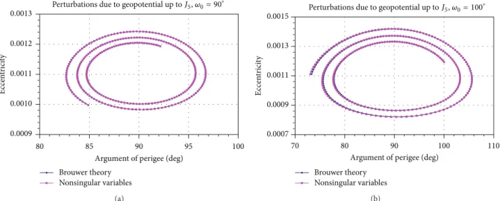
As the analytical development of geopotential and atmospheric drag perturbations may lead to singularities, the equations were rewritten using nonsingular variables approach.Figure 6was built in an efort to verify whether ̇� and ̇�equations were correctly written in terms of nonsingu-lar variables. he results obtained from analytical equations of geopotential up to �₅, that is, developed using Brouwer theory, were compared to the results obtained from the equations written in nonsingular variables. As can be veriied

in Figure 6, the transformation to nonsingular variables

was developed correctly, since the curves plotted extremely resembles. In fact, the curves even superpose each other. And, considering that the interest rests on frozen orbits concept, only�being equal to 90∘and 100∘was considered inFigure 6.

5. Conclusions

(5)

Table 1: Frozen elements maximum variation for each dynamic model.

Initial conditions �₃ �₅ �₃+ drag �₅+ drag

�0 �0 Δ� Δ�(∘) Δ� Δ�(∘) Δ� Δ�(∘) Δ� Δ�(∘)

0.001193 90∘ 2.32E−04 13.583 1.36E−04 7.390 2.31E−04 13.486 1.35E−04 7.322

0.001193 100∘ 3.86E−04 20.195 3.38E−04 16.548 3.83E−04 19.964 3.35E−04 16.360

0.001193 110∘ 6.81E−04 33.496 6.64E−04 29.996 6.76E−04 33.200 6.58E−04 29.728

0.001193 120∘ 1.02E−03 50.737 1.02E−03 46.574 1.01E−03 50.209 1.01E−03 46.111

0.001193 130∘ 1.38E−03 91.747 1.36E−03 73.663 1.36E−03 84.792 1.35E−03 72.323

0.0007 0.0009 0.0010 0.0012 0.0013

60 70 80 90 100 110 120

Eccen

tr

ici

ty

J3

+ J5

�0= 90

∘

(a)

0.0006 0.0008 0.0010 0.0012 0.0014 0.0016

60 70 80 90 100 110 120

Eccen

tr

ici

ty

�0= 100

∘

J3

+ J5

(b)

Figure 3: 300-day phase plane diagram for perturbations due to geopotential up to�₃and�₃+ �₅.

0 40 80 120 160 200 240 280 320

Time (day)

Overlay

Overlay Secular 3.00E − 06

2.00E − 06

1.00E − 06

0.00E + 00

−1.00E − 06

−2.00E − 06

−3.00E − 06

−4.00E − 06

and atmospheric drag

92∘

100∘

�0=

Δe

Δefor perturbations due to geopotential up toJ5

Figure 4: Eccentricity variation in terms of secular and long period components.

were obtained explicitly. To the dynamic model including geopotential up to �₃ terms only were included in pertur-bations due to geopotential up to�₅ and atmospheric drag. he inclusion of such perturbations followed Brouwer and Brouwer and Hori theories. he perturbations analytical expressions were then rewritten in terms of nonsingular vari-ables, in order to avoid singularities due to the eccentricity values used by INPE TSCC. Since the analytical equations

developed for frozen orbits maintenance showed a small additional computational burden, the inclusion of terms due to perturbations of geopotential up to �₅ and atmospheric drag in INPE TSCC operation sotware is justiied.

he inclusion of geopotential perturbations up to�₅was responsible for the major decrease in the frozen elements amplitudes of variation, for any initial condition. he atmo-spheric drag introduces secular and long period components with senoidal outline of exponential overlay amplitude in eccentricity and argument of perigee. Whether to take or not into account the atmospheric drag showed relevant impact for long periods of time.

he frozen elements smaller amplitudes of variation, when �₅ terms and atmospheric drag perturbations are included, improve the precision for prediction of eccentricity and argument of perigee. his means an enhanced precision not only on maneuver’s computations but also on maneuver’s prediction, which contributes to a better performance in the orbital operations conducted at the INPE TSCC.

(6)

0.00 0.05 0.10 0.15 0.20 0.25

0 40 80 120 160 200 240 280 320

Time (day) −0.05

−0.10

−0.15

Overlay

Overlay Secular

Δ�for perturbations due to geopotential up toJ5

and atmospheric drag

92∘

100∘

Δ�

(deg)

�0=

Figure 5: Argument of perigee variation in terms of secular and long period components.

0.0009 0.0010 0.0011 0.0012 0.0013

80 85 90 95 100

Eccen

tr

ici

ty

Brouwer theory Nonsingular variables

Perturbations due to geopotential up toJ5,�0= 90

∘

(a)

Brouwer theory Nonsingular variables 0.0007

0.0009 0.0011 0.0013 0.0015

70 80 90 100 110

Eccen

tr

ici

ty

Perturbations due to geopotential up toJ5,�0= 100

∘

(b)

Figure 6: Comparison between the results obtained analytically and using nonsingular variables approach.

he images from diferent days can be compared for the same latitude and then be used to preview harvests, to detect ire on forests, and to locate underground airports, as well as others utilities.

Appendix

Equations of Motion

he analytical equations for the frozen orbits dynamics, ̇�and

̇�

, which were developed according to Brouwer and Brouwer and Hori theories and were rewritten using nonsingular variables approach are presented as follows:

̇�

= 3��2�2�

�2_{(1 − �}2_{− �}2₎2(1 − 54sin 2_�)

×{{_{_{ {

1 + �3��

2�2� (1 − �2− �2)(

sin2� − ( �2+ �2)cos2�

√�2_{+ �}2_sin_� )

× �

√�2_{+ �}2 +

�5�3� �2�3(1 − �2− �2)3

×{{_{_{ {

5 64[[

[

(( 1 − �2− �2)sin� √�2_{+ �}2 −

√�2_{+ �}2_cos2_�

sin� )

× [4 + 3 ( �2_{+ �}2_{)] + √�}2_{+ �}2_sin_�

(7)

× (1 − 9cos2� − 24cos

4_� 1 − 5cos2�)

− 15₃₂√�2_{+ �}2_cos2_�_sin_{� [4 + 3 ( �}2_{+ �}2_)]

× (3 + 16_{1 − 5}cos_cos2�₂_{� +} 40cos4� (1 − 5cos2�)2)

} } } } }

× �

√�2_{+ �}2 } } } } }

+ � �2�2� 2�2_{(1 − �}2_{− �}2₎2

× (��)1/2exp(−��)

× { −_�₂_{+ �}1 ₂_{(32 −}3₂cos2�)

× [12 + (−24 +1 1112�� + 24�5 2�2) ( �2+ �2) + (−1583_{768 −}233_{128�� −} 3_8�2_�2_{+ 143}

128�3�3 + 13_2304�4_�4_{) ( �}2_{+ �}2₎2_]

+_(�₂_{+ �}₂_{) (1 − �}1 ₂_{− �}₂₎_{(32 −}3₂cos2�)

× [12 + (18 +34�� +18�2�2) ( �2+ �2) + (−667_{768 −} _{192�� +}95 241_384�2_�2_{+ 49}

576�3�3 + 11_2304�4_�4_{) ( �}2_{+ �}2₎2_]

− (32 − 32cos2�)

× [12 + (3124 +1912�� + 24�1 2�2) ( �2+ �2) + (−187_{768 +} _{192�� +}49 123_128�2_�2_{+ 97}

576�3�3 − 5_2304�4�4) ( �2+ �2)2]

− ( 3 −cos2�)

× [(−58 + 14�� +18�2�2) ( �2+ �2) + (− 332 − 16�� −3 16�5 2�2+ 316�3�3

+ 196�4�4) ( �2+ �2)2]

+ [18 (1 − 11cos2� − 40cos

4_� 1 − 5cos2�)

− 5�4 12�2

2 (1 − 3cos

2_{� − 8}cos4� 1 − 5cos2�)]

× [4 + ( 1 + �2_�2_{) ( �}2_{+ �}2₎

+ (− 316 − 38�2�2+ 116�4�4) ( �2+ �2) 2

]

× [18 (1 − 33cos2� − 200cos

4_� 1 − 5cos2� −

200cos6�

(1 − 5cos2�)2)

− 5�4 12�2

2 (1 − 9cos

2_{� − 40}cos4�

1 − 5cos2�

− 80cos6� (1 − 5cos2�)2)]

× [ (1 − ��) (�2_{+ �}2₎

+ (18 + 58�� +18�2�2− 18�3�3) ( �2+ �2) 2

] }

× 2�� √�2_{+ �}2,

̇�

= − 3��2�2�

�2_{(1 − �}2_{− �}2₎2 (1 − 54sin 2_�)

×{{_{_{ {

�3��

2�2�sin� + 532

�5��3 �2�3(1 − �2− �2)3

× [4 + 3 ( �2+ �2)]sin� (1 − 9cos2� − 24cos

4_� 1 − 5cos2�)

× �

√�2_{+ �}2 + 1 − � 2_{− �}2

√�� (�2_{+ �}2₎(−��exp(−��))

× { [1 + (34 + �� +14�2�2) ( �2+ �2)

+ (21_{64 +} 3_{8�� +}_32�9 2�2_{+ 18�}3�3

+ 164�4_�4_{) ( �}2_{+ �}2₎2_] + �2�2�

(8)

× [(12 +78�� +14�2�2− 124�3�3) ( �2+ �2) + ( 21_{256 −} _{256�� +}93 _128�27 2�2+ 39_128�3�3

− 65_768�4_�4_{− 1}

256�5�5) ( �2+ �2) 2

] �_�2₂− �_{+ �}2₂}

+ �2�2� 2�2_{(1 − �}2_{− �}2₎2

×{{_{_{

{[18 (1 − 11

cos2� − 40cos

4_� 1 − 5cos2�)

− 5�4 12�2

2 (1 − 3cos

2_{� − 8}cos4�

1 − 5cos2�)]

× [(32 + 2�� + 12�2�2) ( �2+ �2)

+ (− 316 − 12�� +58�2�2+ 12�3�3+ 116�4�4) × ( �2_{+ �}2₎2_{] �}2− �2

�2_{+ �}2

− ��3 �2

2��sin�

× [(32 + 2�� + 12�2�2) √�2+ �2

+ (−27_{16 −} 5_{2�� +}1_8�2�2_{+ 12�}3�3_{+ 116�}4�4)

× ( �2+ �2)3/2] � √�2_{+ �}2

} } } } } } } } } }

− √ 1 − �_{�� (�}₂2_{+ �}− �₂2₎(−��exp(−��)){{_{

{ {

√ 1 − �2_{− �}2

× [1 + (−14 +14�2�2) ( �2+ �2)

+ (− 364 − 32�3 2�2+ 164�4�4) ( �2+ �2) 2

]

+ �2�2�

2�2_{(1 − �}2_{− �}2₎3/2(32 − 3 2cos2�)

× [(16 +1724�� + 12�5 2�2− 124�3�3) ( �2+ �2) + (−179_{768 −} _{768�� −}7 133_384�2_�2_{+ 311}

1152�3�3 + 95_2304�4_�4_{− 1}

256�5�5) ( �2+ �2) 2

]

× �_�2₂− �_{+ �}2₂ + �2�2� 2�2_{(1 − �}2_{− �}2₎2

× { [18 (1 − 11cos2� − 40cos

4_� 1 − 5cos2�)

− 5�4 12�2

2 (1 − 3cos

2_{� − 8}cos4� 1 − 5cos2�)]

× [(−52 + 2�� +12�2�2) ( �2+ �2)

+ ( 116 −54�� −98�2�2+ 14�3�3+ 116�4�4) × ( �2+ �2)2] �_�2₂− �_{+ �}2₂}

− ��3 �2

2��sin�

× [(−32 + 2�� +12�2�2) √�2+ �2

+ (−27_{16 −} 13_{8 �� −}3_2�2�2_{+ 18�}3�3_{+ 116�}4�4)

+ ( �2_{+ �}2₎3/2_] � √�2_{+ �}2

} } } } } .

(A.1)

Conflict of Interests

he authors declare that there is no conlict of interests regarding the publication of this paper.

Acknowledgments

he authors wish to express their consideration to the National Institute for Space Research (INPE) that kindly provided everything necessary for this paper to be devel-oped. he authors are also grateful to S˜ao Paulo Research Foundation (FAPESP) for the support, under Contract no. 2012/21023-6; to CAPES; and to CNPq.

References

[1] S. L. Cofey, A. Deprit, and E. Deprit, “Frozen orbits for satellites close to an Earth-like planet,”Celestial Mechanics and Dynamical Astronomy, vol. 59, no. 1, pp. 37–72, 1994.

[2] G. W. Rosborough and C. A. Ocampo, “Inluence of higher degree zonals on the frozen orbit geometry,” inProceedings of the AAS/AIAA Astrodynamics Conference, vol. 76, pp. 1291–1304, San Diego, Calif, USA, August 1991.

(9)

[4] M. Ceccaroni, F. Biscani, and J. Biggs, “Analytical method for perturbed frozen orbit around an asteroid in highly inho-mogeneous gravitational ields: a irst approach,”Solar System Research, vol. 48, no. 1, pp. 33–47, 2014.

[5] J. C. Smith, “Analysis and application of frozen orbits for the TOPEX mission,” inProceedings of the AAS/AIAA Astrodynam-ics Conference, AIAA 86-2069, Williamsburg, Va, USA, August 1986.

[6] R. A. Cook, “he Long-term behavior of near-circular orbits in a zonal gravity ield,” in Proceedings of the AAS/AIAA Astrodynamics Conference, pp. 2205–2221, August 1991. [7] E. Cutting, G. H. Born, and J. C. Frautnick, “Orbit analysis for

Seasat-A,”he Journal of Astronautical Sciences, vol. 26, no. 4, pp. 315–342, 1978.

[8] H. Fuming and H. K. Kuga, “CBERS simulator mathematical models,” Tech. Rep., XSCC-Xian Satellite Control Center, 1999. [9] D. Brouwer, “Solution of the problem of artiicial satellite theory without drag,”he Astronomical Journal, vol. 64, pp. 378–397, 1959.

[10] D. Brouwer and G. Hori, “heoretical evaluation of atmospheric drag efects in the motion of an artiicial satellite,”he Astro-nomical Journal, vol. 66, pp. 193–225, 1961.

[11] R. V. de Moraes, “Non-gravitational disturbing forces,” Advances in Space Research, vol. 14, no. 5, pp. 45–68, 1994. [12] S. L. Cofey, A. Deprit, and B. R. Miller, “he critical inclination

in artiicial satellite theory,”Celestial Mechanics, vol. 39, no. 4, pp. 365–406, 1986.

[13] R. Vilhena de Moraes, H. K. Kuga, and P. C. P. Raimundo, “Analytical development of geopotential and atmospheric drag for frozen orbits,” inProceedings of the 5th International Con-ference on Mathematical Problems in Engineering and Aerospace Sciences (ICNPAA ’05), pp. 495–502, Cambridge Publishers, Timisoara, Romania, 2005.

[14] P. C. P. M. Pardal, H. K. Kuga, and R. V. de Moraes, “Study of orbital elements on the neighborhood of a frozen orbit,”Journal of Aerospace Engineering, Sciences and Applications, vol. 1, pp. 23–32, 2008.

(10)

Submit your manuscripts at

http://www.hindawi.com

Hindawi Publishing Corporation

http://www.hindawi.com Volume 2014

Mathematics

Journal of

Mathematical Problems in Engineering

Hindawi Publishing Corporation http://www.hindawi.com

Differential Equations

International Journal of

Volume 2014

Mathematical PhysicsAdvances in

Complex Analysis

Journal of

Optimization

Journal of

Combinatorics

International Journal of

Journal of

Function Spaces

Abstract and Applied Analysis Hindawi Publishing Corporation

International Journal of Mathematics and Mathematical Sciences

Hindawi Publishing Corporation http://www.hindawi.com Volume 2014

The Scientiic

World Journal

Discrete Dynamics in Nature and Society

Discrete Mathematics

Journal of

http://www.hindawi.com Volume 2014 Hindawi Publishing Corporation