Maximilian-Benedikt Herwarth Detlef Köhn
Speculative bubbles and contagion: Analysis of volatility’s clusters during the DotCom bubble based on the dynamic conditional correlation model
Maximilian-Benedikt Herwarth Detlef Köhn
Speculative bubbles and contagion: Analysis of volatility’s clusters during the DotCom bubble based on the dynamic conditional correlation model
SÃO PAULO 2015
Thesis presented to Escola de Economia de Empresas de São Paulo of Fundação Getulio Vargas, as a requirement to obtain the title of Master in Economy.
Knowledge Field:
International Master in Finance
Adviser:
Koehn, Maximilian-Benedikt
Speculative bubbles and contagion: Analysis of volatility’s clusters during the DotCom bubble based on the dynamic conditional correlation model /
Maximilian-Benedikt Koehn - 2015 56.
Orientador: Pedro Luiz Valls Pereira.
Dissertação (MPFE) - Escola de Economia de São Paulo.
1. Crise financeira. 2. Finanças – Aspectos psicológicos. 3. Finanças – Modelos econométricos. 4. Mercado financeiro. I. Pereira, Pedro L. Valls. II. Dissertação (MPFE) - Escola de Economia de São Paulo. III. Título.
Speculative bubbles and contagion: Analysis of volatility’s clusters during the DotCom bubble based on the dynamic conditional correlation model
Thesis presented to Escola de Economia de Empresas de São Paulo of Fundação Getulio Vargas, as a requirement to obtain the title of Master in Economy.
Knowledge Field:
International Master in Finance
Approval Date: ___/___/____.
Committee members:
_________________________________ Prof. Dr. Pedro Luiz Valls Pereira
_________________________________ Prof. Dr. João Pedro dos Santos
Sousa Pereira
Dedicated to the “Seven Fs”:
Faith, Family, Finances, Fitness, Friends, Fun and Future by
Revendo a definição e determinação de bolhas especulativas no contexto de contágio, este estudo analisa a bolha do DotCom nos mercados acionistas americanos e europeus usando o modelo de correlação condicional dinâmica (DCC) proposto por Engle e Sheppard (2001) como uma explicação econométrica e, por outro lado, as finanças comportamentais como uma explicação psicológica. Contágio é definido, neste contexto, como a quebra estatística nos DCC’s estimados, medidos através das alterações das suas médias e medianas. Surpreendentemente, o contágio é menor durante bolhas de preços, sendo que o resultado principal indica a presença de contágio entre os diferentes índices dos dois continentes e demonstra a presença de alterações estruturais durante a crise financeira.
Reviewing the definition and measurement of speculative bubbles in context of contagion, this paper analyses the DotCom bubble in American and European equity markets using the dynamic conditional correlation (DCC) model proposed by Engle and Sheppard (2001) as an econometrical - and on the other hand the behavioral finance as an psychological explanation. Contagion is defined in this context as the statistical break in the computed DCCs as measured by the shifts in their means and medians. Even it is astonishing, that the contagion is lower during price bubbles, the main finding indicates the presence of contagion in the different indices among those two continents and proves the presence of structural changes during financial crisis.
TABLE OF CONTENTS
TABLE OF CONTENTS ... 8
LIST OF TABLES ... 9
LIST OF FIGURES ... 9
LIST OF ABBREVIATIONS ... 10
1. INTRODUCTION ... 11
2 OVERVIEW OF RELEVANT LITERATURE ... 13
2.1 PRICE BUBBLES ... 13
2.2 FINANCIAL CONTAGION ... 14
3 PRICE-BUBBLES AND THEIR IDENTIFICATION ... 17
3.1 INTRODUCTION AND DEFINITION ... 17
3.2 TYPICAL DEVELOPMENTS OF BUBBLES ... 19
3.3 TECHNOLOGY-BUBBLE AND THEIR DEVELOPMENT ... 20
3.4 BEHAVIORAL FINANCE ... 23
3.4.1FEEDBACK TRADING MODEL ... 23
3.4.2OTHER BEVAVIORAL EXPLANATIONS ... 26
4 METHODOLOGY AND EMPIRICAL SPECIFICATION ... 27
4.1 DATA ... 27
4.2 DESCRIPTIVE STATISTICS ... 29
4.3 MODEL SPECIFICATIONS ... 31
5 EMPIRICAL RESULTS ... 34
6 SUMMARY & CONCLUSION ... 40
7 REFERENCES ... 42
LIST OF TABLES
TABLE1. OVERVIEW OF EMPIRICAL RESEARCHES………..…16
TABLE2. DESCRIPTIVE STATISTICS OF COMPOUNDED STOCK MARKET RETURNS…...30
TABLE3. UNIT ROOT TESZS: ADF, PP AND KPSS………...31
TABLE4. OBTAIN LAG-ORDER SELECTION STATISTICS………...34
TABLE5. DYNAMIC CONDITIONAL CORRELATION………..35
TABLE6. CONSTANT CONDITIONAL CORRELATION………52
TABLE7. VARYING CONDITIONAL CORRELATION………..52
TABLE8. DYNAMIC CONDITIONAL CORRELATION DOTCOM………...53
TABLE9. CONSTANT CONDITIONAL CORRELATION DOTCOM………..53
TABLE10. VARYING CONDITIONAL CORRELATION DOTCOM………..54
TABLE11. WALD TEST………....36
TABLE12. WALD TEST FOR DOTCOM TIME FRAME……….46
TABLE13. DYNAMIC CONDITIONAL CORRELATION- SAMPLE VS DOTCOM………….37
TABLE14. CONSTANT CONDITIONAL CORRELATION- SAMPLE VS DOTCOM…………54
TABLE15. VARYING CONDITIONAL CORRELATION- SAMPLE VS DOTCOM…………..55
LIST OF FIGURES FIGURE1. STOCHASTIC AND DETERMINISTIC BUBBLES………..18
FIGURE2. NASDAQ COMPOSITE AND OMPOUNDED NASDAQ COMPOSITE 1990-2005………..22
FIGURE3. AMERICAN AND EUROPEAN INDICES 1990-2005………...……22
FIGURE4. NORMALIZED STOCK MARKET INDICES………..28
FIGURE5. ALL STOCK MARKET INDICES……….50
FIGURE6. STOCK MARKET INDICES………50
FIGURE7. STOCK MARKET RETURNS………..29
FIGURE8. SCATTER PLOT EVERY INDICES WITH EACH OTHER………51
FIGURE9. ESTIMATED DYNAMIC CORRELATION COEFFICIENTS……….…38
FIGURE10. CONDITIONAL VARIANCES OF THE RETURNS………...39
FIGURE11. ESTIMATED DYNAMIC CORRELATION DOTCOM………55
LIST OF ABBREVIATIONS
ADF Augmented Dickey-Fuller
AIC Akaike’s Information Criterion
ARCH Autoregressive Conditonal Heteroskedasticity
CCC Constant Conditional Correlation
Coef. Coefficient
Conf. Int. Confidence Interval
DAX Deutscher Aktienindex (German Stock Index)
DCC Dynamic Conditional Correlation
e.g. exempli gratia (for example)
et. al. et alii (and others)
FPE Final Prediction Error
FTSE100 Financial Times Stock Exchange
GARCH Generalized Autoregressive Conditional Heteroskedasticity
HQIC Hannan and Quinn Information Criterion
INDU Dow Jones Industrial Average
IXIC NASDAQ Composite
KPSS Kwiatkowski, Phillips, Schmidt, and Shin
MGARCH Multivariate Generalized Autoregressive Conditional Heteroskedasticity
NASDAQ National Association of Securities Dealers Automated Quotations
SBIC Schwarz’s Bayesian Information Criterion
SP500 Standard & Poor's 500
SXXE EURO STOXX Index
Std. Err. Standard Error
PP Phillips-Perron
1. INTRODUCTION
The deviation of market prices from fundamental values is not only a
phenome-non of the present, but is also observed since the last centuries, e.g.: The Tulipomania in
Netherlands, the South Sea Bubble in Great Britain or even the DotCom bubble, see
Carlos et al. (2006) or Ofek and Richardson (2003).
During those last centuries, the analysis of patterns of international spread of financial
events became the subject of many academic studies. Especially, during price-bubbles,
empirical research focused on volatility models and tried to answer the international
markets’ phenomena of high correlated markets.
De facto, financial markets around the world are getting more and more integrated. In
those highly integrated markets any shock in a single market can quickly lead to a
spill-over to other markets. The reason behind this can have different sources, for instance:
financial, geopolitical, and political relations between those countries. Empirical studies
of contagion events, which focus only on the fundamental relations among economies,
are not able to explain satisfactorily those spillovers from one market to another. The
behavioral finance theories offer a behavioral-psychological explanation for those
dif-ferent stock market anomalies and their spillover effects. Shock spillovers and thereby
contagion can be attributed to irrational behavior of investors and for instance linked to
a herding behavior among them, shown by Hirshleifer and Teoh (2009) and Ionescu et
al. (2009).
The term contagion has been gone through a lot of different definitions and
measurements, always trying to define and answer the process in a context of
cross-country analysis. In the beginning, it was defined as a simple static measure of
transferred the relation to their respective equity markets and to a cross-country
portfo-lio diversification, shown by Cho and Parhizgari (2008). Later on, researches – like
Darbar and Deb (1997), Karolyi and Stulz (1996), and Parhizgari et al. (1994) – on
cor-relation analyses tried to develop new measures and techniques by including
co-movements, causality and error-correction models among cross-country market returns.
Meanwhile, like Forbes and Rigobon (2002) have shown, the estimation of
cor-relations requires additional statistical refinements. Engle and Sheppard (2001)
demon-strated that those estimations have to consider the dynamics - the time-varying and the
constant - aspect of correlations, which is called dynamic conditional correlations
(DCC).
In consideration of previous studies, this paper answers the following questions
and closes thereby a rarely mentioned topic in the literature about the correlation of
market indices and the evaluation of financial contagion between stock-market returns:
1. What is a speculative bubble and how can be indicated a typical price bubble?
2. Holds the - in many cases assumed - contagion effect between the American
and European stock markets in the presence of price bubbles, like the DotCom
bubble?
3. Which model is the best for analyzing the phenomenon of financial contagion
between stock market returns of different countries?
In this context, the goals of this study are to analyze the DotCom price bubble as
well to evaluate the financial contagion between American and European stock market
returns in this context. Therefore, three multivariate conditional correlation volatility
models will be used, the DCC-GARCH by Engle and Sheppard (2001), the constant
correla-tion (VCC) by Tse and Tsui (2002). Nevertheless, the main focus lies on the
DCC-GARCH model.
The paper is constructed as follows: Chapter 2 gives a short overview about the
literatures of price bubbles and financial contagion. Chapter 3 defines generally
price-bubbles and their development, subsequently the DotCom bubble is explained as well
shortly analyzed. The chapter 4 starts with a short descriptive statistic of the considered
data set and describes the empirical strategy according to test for financial contagion.
Chapter 5 presents the results according to previous strategies and the last chapter
con-cludes and compares the results with former findings.
2 OVERVIEW OF RELEVANT LITERATURE
According to the different parts of this study, the overview of relevant literature
has to be split as well into two main parts: The first part deals with the definition of
bubble and their different explanations. The second part deals about the contagion effect
among the different indices.
2.1 PRICE BUBBLES
The discussion how to define and identify a bubble is not a new topic. Garber
(2000)explains a bubble as “a fuzzy word filled with import but lacking any solid
oper-ational definition.” He defines both sides of a bubble, the positive as well as the
nega-tive. He suggests that a bubble can best be explained by “a price movement that is
inex-plicable based on fundamentals.” The main task of this definition is that a bubble can
in-stance, Kindleberger and Aliber (1996) defines that “a bubble is an upward price
movement over an extended range that then implodes.” The most important
assump-tions to define a bubble are the irrationality versus the rationality. Arrow (1982) gives a
short summary over the difference between individual rationality and irrationality and
markets.
Blanchard and Watson (1982) published one of the first papers about bubbles in the
financial markets regarding the rational expectations. The more recent paper by O’Hara
(2008) summarized the overview of literature about bubbles in detail. In her paper, she
distinguished different theories of bubbles. Therefore, she differentiated between
ration-al and irrationration-al traders, as well rationration-al and irrationration-al markets. Tirole (1982) and
Brun-nermeier and Nagel (2004) showed that a bubble could even occur under the assumption
of rational investors and rational markets. The theory behind the irrationality of the
markets is based on the theory of Kindleberger and Aliber (1996) and Keynes (1935).
This paper analyzes the technology-bubble – often mentioned as the DotCom-bubble.
Ofek and Richardson (2003) were one of the first authors, who explained the internet
bubble in the 1990’s. Their conclusion is that the technology-bubble “burst to the
un-precedented level of lockup expirations and insider selling”. This study assumes also
rational markets, like Ross (2005) and Aschinger (1991) did. Garber (1990) gives a
good overview over the past famous bubbles and concludes that a bubble is a present
phenomenon and will occur frequently.
2.2 FINANCIAL CONTAGION
The literature about contagion effect in financial markets is that extensive to
et al. (2003) are only some of those, which have to be mentioned. In general, the focus
of most literatures is the contagion effect across countries. Therefore, the spread of
cri-ses from one country to another has been one of the most discussed issues in
interna-tional finance since the last decades. This is caused by the frequently occurrence of the
last crisis. Financial contagion characterizes situations in which local shocks are
trans-mitted to others financial sectors or even countries. This is comparable with a pandemic,
for instance an epidemic of infectious disease. One of the most known definition
ex-plains a contagion as a “structural change in the mechanism of the proliferation of
shocks arising from a particular event or group of events associated with a particular
financial crisis”; see Arruda and Pereira (2013). Applied to a financial crisis means this
that a specific shock can propagate like a virus, starting in a country and overlapping
even to other continents.
An interesting way to define contagion is the five-step definition by Pericolo and
Sbracia (2001). According to the authors, contagion can be explained by a) an increased
probability of a crisis in a country by a crisis in another - different - country; b) highly
stock volatility as an uncertainty from crisis of a country to the financial market of
an-other country; c) higher co-movements in stock prices or quantities between financial
markets with and without crisis in the markets; d) difference in transmission mechanism
or channel for contagion in and after the crisis; and e) co-movements which can not
explained by the fundamentals.
For instance, Filleti et al. (2008) analyzed the contagion between the Latin American
economies and two emerging markets. Armada et al. (2011) tested the contagion effect
between the financial markets of nine developed countries and Azad (2009) for the
contagion effects during the US Subprime crisis. Marcal et al. (2011) evaluated the
con-tagion in the financial crisis of Asia and Latin America.
Regarding to the technology-bubble, Anderson et al. (2010) studied the proliferation of
the technology-bubble. Most of the studies applied variations of Engle and Sheppards’
(2001) DCC model. Table 1 gives a short overview about the different researches,
which mainly focus on the effect of financial crisis on emerging markets.
TABLE 1: OVERVIEW OF EMPIRICAL RESEARCHES
None of the previous studies analyzed only the contagion effect between
Ameri-can and European indices during the technology-bubble, most of the studies related the
contagion between developing, industrialized and emerging countries.
Consequently, this paper will confirm the hypothesis of financial contagion
dur-ing the technology-bubble, if structural breaks are identified. In contrast to previous
which analyzed the financial contagion among several industry-sectors in a specific
country, this paper will focus on the contagion within different countries during the
technology-bubble. The presence of a contagion effect can be determined by the
in-crease in conditional correlations of the indices during the period of crisis compared to
the previous periods.
3 PRICE-BUBBLES AND THEIR IDENTIFICATION
“A market in which prices always fully reflect available information is called efficient“, by Fama (1970)
3.1 INTRODUCTION AND DEFINITION
As mentioned before, many papers focus on the explication, proof and analysis
of market mispricing. Particularly, many well-known scientists - leading by Shiller
(2000) and Fama (1965) - are engaged in the detection of bubbles. There are different
opinions how to define a price-bubble. There are two kinds of bubbles: The
determinis-tic bubble, which will burst in a specific time or the stochasdeterminis-tic, which will increase to
infinite, as seen in figure 1. Trivially said and knew from the efficient-market
hypothe-sis of Fama (1970): An investor cannot score abnormal returns, because all relevant and
available information are included in stock prices.
Nevertheless, at the beginning of every speculative price-bubble there is a belief
of high probability of excess returns, see therefore Garber (1990). In an efficient
mar-ket, stock-market changes are only justified with new information. During the
normally no new information are published, which could explain those high
stock-prices.
Notwithstanding, one of the most-known definitions is following: A positive
price-bubble is the deviation of market price from the expected discounted dividends
(this is called the fundamental value) and is based on the dividend model of William
(1938):
�!>
!(!!)
!!! !!!
!
!!! (1)
�! defines market price, �! dividends and returns. Speculative bubbles can arise from
stock’s price-expectation. As mentioned before, there are two types of bubbles. The
main focus of this paper, as those of Scherbina (2013), Jarchow (1997), will be
stochas-tic bubbles. Those can burst with a specific probability during the time-period. In
con-trast to stochastic bubbles, deterministic bubbles increase to infinite. If a bubble burst,
there are two following opportunities:
1) The market price will fall behind in the fundamental value, or
2) the market price will fall below the fundamental value.
Figure 1, based on the theory of Aschinger (1991) and Jarchow (1997), shows the
dif-ferent two scenarios: a deterministic Bdet and a stochastic bubble (Bstoch) under the
as-sumption that the fundamental value stays constant during time.
FIGURE 1.STOCHASTIC AND DETERMINISTIC BUBBLES
3.2 TYPICAL DEVELOPMENTS OF BUBBLES
The majority opinion about a typically development of a bubble is based on
Kindleberger and Aliber (2005), Rosser et al. (2012) and Aschinger (1991). Below, the
characteristics and phases of a speculative bubble are illustrated generally - as well -
compared to the technology-bubble:
1) The beginning of each bubble is initiated with an exogenous shock, which
implicates pervasive economical changes. In this phase a full branch of an industry can
be changed. The exogenous shock can be caused by economical or political reasons;
some are even caused by new technological developments. Structural changes raise the
optimism of investors, banks and companies. The optimism and the expectation of a
new welfare and new expected profit of the companies encourages investments to risky
stocks. The expectation of stock market is positive. Therefore, investors hope for higher
returns than in status quo ante.
2) The next step of a speculative bubble - the boom - is reached by the
expecta-tion of always continuing raising returns and a potential new market. By dint of
equa-tion 1 means that, that the market price is now a multiple of its proper fundamental
val-ue.
3) In consequence to the phase of the boom, interest rates are generally reduced,
credit activities are increased and therefore, the total money supply increases. This
be-havior intensifies the proper boom-phase. The demand for credit increases permanently.
4) The abnormal increase of the stocks allures speculators and the credit
activi-ties are expanded by lower interest rates. A perpetual growing spectrum of participants
from wealthy investors, debt-financed investors, and in the end speculators
5) A disproportionately high return-expectation arouses even more investors,
who are investing even more capital in the price-bubble. In this phase behavioral and
irrational factors determine the investors’ buying behavior. For instance, bandwagon
effects are incorporated into behavioral effects: Following the motto, if others are
buy-ing, I will also buy. Those herd instincts happen avalanche-like and increase the capital
inflow of each bubble, as Weil (2010) showed.
6) Due to higher interest rates, stagnant price trends or rejection of new
technol-ogies- the expectation can dramatically change. The first disembark of insiders, who
would like to liquidate their winnings, triggers speculations of declining stock prices.
7) Professional investors escape. The others, the much bigger mass of
non-professional investors, are trying to liquidate their winnings as well. This will lead to a
huge increase of the demand of liquids funds in fear of illiquidity. The mass gets into a
kind of a panic and sells their stocks at any price. Because the order of selling
domi-nates, the prices will decline strongly. The speculative bubble burns, and the prices will
go back to their fundamental value. This is caused to the microeconomic model supply
and demand; stock prices will decrease at oversupply.
3.3 TECHNOLOGY-BUBBLE AND THEIR DEVELOPMENT
The following chapter will give a short overview about the technology-bubble –
also called DotCom bubble because of the domain ending COM – and analyze it with
the help of the previous shown development.
The technology-bubble started not at a fix time, it grew during the early 90’s
The start of the technology-bubble was caused by the hope, that the internet can
im-prove the productivity of a company and therefore increase their expected profits.
As Xiong (2013) and Scherbina (2012) have shown the interest of achieving excess
re-turns grew in times of the technology boom, especially of private investors.
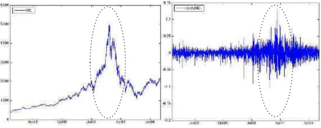
The chart of the index NASDAQ gives a good overview of this speculative
bub-ble: The NASDAQ increasedsince the end of the 90’s. It doubled up in the time period
between 1996 and 1998 and even quadrupled in the time between 1998 and 2000.
Espe-cially during the technology-bubble, the demand of internet-companies was enormous,
whereupon the expected profit, respectively the winning-probability, of those
compa-nies were excluded and evaluated even illusory. The basic idea behind the trade of those
stocks was trivially: One thought that the companies would offer their services for free
at the beginning, thus would improve their market share and would generate some sales
at a future date. Many of those new founded companies had the same business-idea and
competed against each other. The technology-bubble burst in March 2000. Analog to
the foundation of many new companies with similar business-ideas and their parallel
increase in stock-prices, many of those companies moved avalanche-like - as well - to
the other direction up to bankruptcy in March 2000. Discussed by Scherbina (2012),
Ofek and Richardson (2003), Xiong (2013) and Brunnermeier and Nagel (2004) as well.
Figure 2 shows on the left hand the NASDAQ Composite (IXIC) as well on the right
hand the compounded NASDAQ Composite. Those figures illustrate exemplary the
FIGURE 2. NASDAQ COMPOSITE AND COMPOUNDED NASDAQ COMPOSITE 1990-2005
The technology-bubble triggered an enormous worldwide financial crisis and
showed the influences of overoptimistic perspectives for the Internet industry and
there-fore, the high stock prices. Figure 3 shows the INDU, DAX, FTSE100, SP500, SXXE,
and IXIC. The graph shows the series with all indices normalized to 100 points on the
first day of the sample, 1 December 1990. The indices are normalized to illustrate better
the relative performance of the initial value of each index.
FIGURE 3. AMERICAN AND EUROPEAN INDICES 1990-2005
As one can see, all graphs have a similar trend and the series are not stationary.
bubble is different. For instance, some markets are highly volatile, like IXIC or SXXE,
others like FTSE100 shows a more stationary trend behavior.
Nevertheless, one can identify some volatility cluster and show that this holds even for
the compounded returns - as will be shown later on in chapter 4.
3.4 BEHAVIORAL FINANCE
A main important part of the puzzle of a speculative bubble is the assumption of
a Homo Oeconomicus, a fully rational individual. But especially individuals, like
inves-tors, tend to overreact or make decision regarding irrelevant information’s. This is in
contrast to the assumption of a full-rational investor, who will always make rational,
utility-maximizing decisions, like Sheffrin (1983) and Simon (1979) point out. This
irrational behavior tends to result in excess volatility clusters. Therefore, to understand
more in detail which physiological factors drive a bubble, this chapter will focus on the
behavioral finance and analyze those with the dotcom-bubble. The behavioral finance is
a new behavioral-scientific approach, which explains stock volatilities during
specula-tive bubbles with the help of psychologies and rational models. Employing
behavioral-scientific approaches, the processing of relevant information’s are analyzed to explain
speculative bubbles. (Nguyen and Schueßler 2011)
3.4.1 FEEDBACK TRADING MODEL
One of the main discussed models of the behavioral finance is the Feedback
Trading model at the stock market. This model produces a speculative bubble under the
trading information’s. The mechanism of those models allows a bubble to grow with
more capital inflow until a certain time. At the moment when the capital inflow will
rapidly decrease, the bubble will break down.
The following example will explain this theory:
Caused by positive news of a company their stock price increases. Some
inves-tor groups buy those stocks with the expectation that the stocks will increase in the
fu-ture and therefore, the return increases as well. The first step is to define the trading
volume as the amount of trading stocks of those companies. The demand after those
stocks increases with the expectation of growing returns and involving that the stock
price will be higher than the fundamental value. The trading volume increases also
be-cause of the amount of money. Those will attract as well other Feedback Traders, who
are expecting that the price will still grow. This schematic repeats as long as no capital
is invested anymore. At this point, the price will not grow anymore. Investors would
like to sell their stocks profitably. The necessary demand of capital threatens the
bub-ble- it can and will burst, see Scherbina (2013) for more details.
A bubble will burst therefore, when the supply of capital is exhausted. To grow a
speculative bubble need to get more new invested capital. Once the capital inflow will
decrease, the prices will fluctuate. The result of this will change the optimistic mood,
which will deflate the bubble as well. In fact, there are some indicators that a bubble
will burst as soon as a huge amount of unprofessional investors are speculating with
those overpriced stocks, as Scherbina (2013) showed.
Many behavioral models assume that competitive arbitragers limit the huge price
volatilities. The following model by De Long et al. (1990a) shows that rational
model implies three investor types, based on DeLong et al. (1990a) and Scherbina and
Schlusche (2012):
1) Positive Feedback Trader: The base of the stock demand is based only on
past prices changes.
2) Passive Trader: The trading base is dependent on the asset value relative to
their fundamental value.
3) Informed rational speculators: The foundations of their trading’s are news
about the fundamental value as a hypothesis for future price movements.
With the help of those models Belhoula and Naoui (2011) showed that rational
investors tend to destabilize than to stabilize stock prices. One assumption is that the
rational investors know the Feedback Traders based their future demand on the base of
past price changes. To get higher price volatility, speculators have a higher demand of
trading than in absence of Feedback Trader. If Feedback Traders entrance the market,
the speculators invert their trading’s and earn the profit from the Feedback Trader’s
expense.
The model shows clearly that rational speculators are not trading against
ex-pected future mispricing’s, which occurs as a result of an overreaction of the Feedback
Traders to past prices changes. Instead, rational speculators anticipate the behavior of
positive Feedback Traders and drift the prices up. In following rational trader will gain
from those mispricing’s and buy the stocks to sell those later to inflationary prices. The
rational arbitragers will benefit from the bandwagon effect instead of trading against the
mispricing’s. All in all, a bubble arises from those rational, speculative behaviors.
Those findings coincide with the conclusions of Abreu and Brunnermeier (2003) and
3.4.2 OTHER BEVAVIORAL EXPLANATIONS
This following section will discuss some more behavioral aspects to understand
better the behavioral explanation of a speculative bubble. Overconfidence and over
op-timism are important for the evaluation of stock prices, as De Bondt (1998) found out.
Individuals tend to be overoptimistic if they have an own influence on stock prices. The
phenomenon of overconfidence explains that every individual has a higher confidence
in his own expectation and evaluation. Both phenomena’s are documented by
experi-ments: Stocks, which are held in their own portfolios, are getting overvaulted belong
their returns and expected growth.
Another effect is called the bandwagon effect or as well the herding behavior,
based on DeBondt and Forbes (1999). This phenomenon explains the buying behavior,
which is influenced by the buying behaviors of others. This means: A non-professional
investor buys/sells stocks analog to the market/investors-majority in a speculative
bub-ble. He makes his decision based on other market participants, which emblematize the
majority. This behavior is relevant: On the right hand, he does not deviate from the
ma-jority opinion, because the mama-jority cannot be wrong. On the other hand, he is not
will-ing to swim against the stream and be against the majority. Nguyen and Schueßler
(2011) analyzed this specific behavior.
Another aspect that occurs during a bubble is the Narrow Framing, researched and
troduced by Barberis and Thaler (2002) and Barberis et al. (2006). This means that
in-dividuals judge differently over identical stocks in the same decision situations, if the
stock or portfolio strategy is positive described. In the initial stage of the
technology-bubble one assumed a huge benefit of new technology innovations. In those times
technologies, get an even higher rating than if they were objective rated.
Non-professional investors tends also to hold bad-performed stocks to long, so that, they do
not have to realize their loses. That loss-aversion affects the behaviorism of each
inves-tor.
To understand the formation phase of a speculative bubble you have to take
those previous behaviors in consideration. Under rational assumption, it does not make
sense to invest in stocks, which have a higher market value than their fundamental
val-ue. But this happens explicit during bubbles as shown by Weil (2010) and as well by
Nguyen and Schueßler (2011). Non-rational investing means not only that stock prices
are determined not always objective by future expectations but also biased by individual
characters and their emotional factors, as respectively shown by the studies of Barberis
et al. (2006), Kugler and Hanusch (1992).
4 METHODOLOGY AND EMPIRICAL SPECIFICATION
In following chapter, the data set will be analyzed as well as the dynamic
condi-tional correlation (DCC) model will be explained.
4.1 DATA
The data on stock market prices consists of the Standard and Poor's 500 (SP500),
Dow Jones Industrial Average (INDU), NASDAQ Composite (IXIC), Financial Times
Stock Exchange (FTSE100), Deutscher Aktienindex (DAX) and Euro STOXX Index
(SXXE) for U.S., U.K. and Germany. (All indices are shown in figure 6 in the
repre-sentatives for American and as well three for European markets. The daily data are
col-lected over the period from December 1, 1990 to December 31, 2014.
All data are obtained from Bloomberg. Daily data are used in order to retain a high
number of observations to adequately capture the rapidity and intensity of the dynamic
interactions between markets.
Figure 4 presents the normalized stock market indices with an interesting
pat-tern. Using normalized stock market prices; the figure illustrates better the relative
per-formance of the initial value of each index than plotting all indices naturally, as seen in
Figure 5 in the Appendix. Figure 4 identifies a period of joint fall in all the indices
con-centrated during the highlighted period (from July of 1998 to October of 2001).
FIGURE 4. NORMALIZED STOCK MARKET INDICES
Regarding the sample definition, the intention was to select an extensive set of
historical data with approximately a 24-year period, which amounted to 5952
observa-tions for each series. Compounded market returns i (index i) at time t are computed as
following:
�!,!= log(
!!,!
!!,!!!
where �!,!and �!,!!! are the closing prices for day t and t −1, respectively. Figure 7
in-dicates those compounded market returns and identifies some clusters, especially in
times of crisis and bubbles. As Figure 7 clearly shows, the volatility cluster during the
DotCom period seems to be more sprawled than the subprime crisis, which had highly
returns in a short-term.
FIGURE 7. STOCK MARKET RETURNS
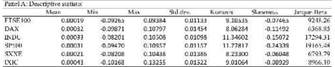
4.2 DESCRIPTIVE STATISTICS
The descriptive statistics of the data are given in table 2, which is divided in two
panels A and B. As seen from panel A, the mean value for each return series is close to
zero and for each return series the standard deviations are larger than the mean values
and varies from 1.05% to 1.45%. The minimum alters from -8.20% to -10.17% and the
maximum varies from 9.38% to 13.26%. Each compounded market return displays a
to 11.78 - indicating that there are bigger tails than the normal distribution and
there-fore, the returns are not normally distributed.
In panel B, unconditional correlation coefficients in stock market index returns indicate
strong pairwise correlations. The correlations within the different continents are highly
positive over the full sample. The European indices: FTSE100, DAX and SXXE, have a
correlation between 76% to 90% and the American Indices: INDU, SP500 and IXIC,
have nearly 78% to 96%. The correlations between the different continents are even
high; every correlation is bigger than 44%. Those high positive unconditional
correla-tions are the first indicators for a strong contagion effect.
TABLE 2.DESCRIPTIVE STATISTICS OF COMPOUNDED STOCK MARKET RETURNS
The results of the unit root tests for the market returns are summarized in table 3.
The Augmented Dickey-Fuller (ADF), Phillips-Perron (PP) and Kwiatkowski, Phillips,
Schmidt, and Shin (KPSS) tests are used to explore the existence of unit roots in
indi-vidual series. The results of unit root tests have rejected the null hypothesis of the unit
TABLE 3.UNIT ROOT TESTS:ADF,PP AND KPSS
Figure 8 depicts the plots between every indices. Visually, one can see a higher
relationship between indices from the same continent, for instance SP500 and INDU, or
DAX and SXXE. It is not a perfect relationship, because not all points are lying exactly
on the straight lines. The closer they are to the line (taken altogether), the stronger
would be the relationship between the variables. These relationships between the series
are linearly fitted by straight red lines.
4.3 MODEL SPECIFICATIONS
The econometric method is based on the modeling of multivariate time-varying
volatilities. One of widely used models is DCC one of Engle and Sheppard (2001) and
Tse and Tsui (2002), which captures the dynamic of time-varying conditional
correla-tions, contrary to the benchmark CCC model by Bollerslev (1990) which keeps the
con-ditional correlation constant. The main idea of this models is that the covariance
trix,�!, can be decomposed into conditional standard deviations, �!, and a correlation
matrix,�!. �!as well �! are designed to be time-varying in the DCC GARCH model.
The specification of the DCC model can be explained as follows:
�! =�+ �!
!
!!! �!!!+�! ���� =1,…,�����! Ω!!!~�(0,�!), (3)
where �! is a 6×1 vector of stock market index returns.
follows with z is a 6×1 vector of i.i.d errors:
�! = �!"#$!"!,!,�
!"#,!,�!"#$,!,�!"!"",!,�!""#,!,�!"!#,! !
= �! !
!�
! (4)
���ℎ�!~�(0,�!).
�!is the conditional covariance matrix and is given by following equation:
�! =�(�!�!′Ω!!!). (5)
Therefore, equation can be written for the 6 different market indices:
�!"#$!"",! �!"#,! �!"#$,! �!"!"",! �!""#,! �!"!#,!
=
�!"#$!""
�!"#
�!"#$ �!!!"" �!""# �!"!#
+
�!!! �!"! �!"! �!"! �!"
!
�!"! �!"! �!!! �!"! �!"! �!" ! �!"! �!"! �!"! �!!! �!"! �!"! �!" ! �!"! �!"! �!"! �!!! �!"! �!"! �!" ! �!"! �!"! �!"! �!! ! �!"! �!" ! �!" ! �!" ! �!"! �!"! �!! ! ! !!!
�!"#$!"",!!!
�!"#,!!!
�!"#$,!!!
�!"!"",!!!
�!""#,!!!
�!"!#,!!!
+
�!"#$!"",!
� !"#,! �!"#$
,! �!"!"",!
�!""#,!
�!"!# ,!
. (6)
Applying Engle and Sheppards’s 2001 dynamic conditional correlation model, the
�! = �!"#$!"",!,�!"#,!,�!"#$,!,�!"!"",!,�!""#,!,�!"!#,! !
is a 6×1 vector of stock market
returns, such that �!"#$!"" is the return of FTSE 100, respectively the other indices with
�! Ω!!!~�(0,�!).
The conditional covariance matrix �! is defined by two components on the CCC model,
which are estimated independent of each other: The sample correlations �! and the
di-agonal matrix of time varying volatilities �!. Therefore, the covariance forecast is given
by following equations:
�! =�!�!�!, (7)
where �! =���� ℎ!"#$!"",!, ℎ!"#,!, ℎ!"#$,!, ℎ!"!"",!, ℎ!""#,!, ℎ!"!#,! is a
6×6 diagonal matrix of time varying standard deviations from the univariate GARCH
models, for
ℎ!,! =�!+�!�!,!!!!+�!ℎ!,!!! (8)
correlation matric is defined by:
�! = �!,! . (9)
Getting the DCC-GARCH model, two steps have to be taken. The first one is to
esti-mate a univariate GARCH model. The second stage is to define the vector of
standard-ized residuals, �!,!=
!!,!
!! ,!
to develop the DCC correlation specification:
�! =���� � !! !!! ,… ,�!!! ! ! � !���� � !! !!! ,…,�!!! !
! , (10)
where �! =(�!,!,!) is a symmetric - positive defined - matrix. �! varies according to a
GARCH-type process as follows:
�! = 1−�! −�! �+�!�!!!�!!!!+�!�!!! (11)
The variables, �
! and �!, are positive,�! ≥ 0����! ≥0 and, therefore, �! +�! <1.
�
!��� �! define scalar parameters, which capture the effects of previous shocks and
previous dynamic conditional correlation on current dynamic conditional correlation. �
explains the 6×6 unconditional variance matrix of all standardized residuals �!
,! with
a correlation estimation like following:
�!,!,! = !!,!,!
!!,!,!!!,!,!
≤ 1 (12)
As Aielli (2013) pointed out in the DCC model the choice of � is not obvious as �! is
neither a conditional variance nor correlation, even �(�!!!�!!!!) seems to be
incon-sistent for the target because of �! not having a martingale representation. Aielli (2013)
solved the issue of the lack of consistency and the existence of biased estimation
pa-rameters by introducing a corrected DCC model (cDCC). This model has nearly the
same specification as Engel’s (2002) DCC model, except the correlation �!:
�! = 1−�!−�! �+�!�!∗!!�∗!!!
! +�
!�!!!,���ℎ�∗ = ���� �! !
5 EMPIRICAL RESULTS
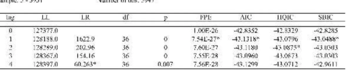
Table 4 reports the final prediction error (FPE), Akaike’s information criterion
(AIC), Schwarz’s Bayesian information criterion (SBIC), and the Hannan and Quinn
information criterion (HQIC) lag order selection statistics for a series of vector
auto-regressions of order 1 through a requested maximum lag. The equation for the FPE is
given by Luetkepohl (2005), with T as the number of observations and K as the number
of equations:
��� = Σ!
!!!"!!
!!!"!!
!
(14)
AIC, SBIC and HQIC are computed according to their standard definitions, see fore
those equations Akaike (1974), Schwarz (1978) and Hannan and Quinn (1979):
��� =−2 !! ! +
!!!
! (15)
���� =−2 !!
! +
!" (!)
! �! (16)
���� =−2 !!
! +
!"# (!"! )
! �!, (17)
where LL is the log likelihood and �
! indicates the total amount of parameters in the
model.
Table 4 is the result as preestimation. This preestimation version is later used to
select the lag order for the three different MGARCH-models.
The “*” indicates the optimal lag. Even, the FPE is not an information criterion;
the prediction error has to be minimized. Therefore, it is included in the lag selection
discussion and is selected by the lag length with the lowest value. Measuring the
differ-ence between given model and true model, the AIC has to be as low as possible, shown
by Akaike (1973). A similar interpretation provides the SBIC and the HQIC.
Luet-kepohl (2005) discussed the theoretical advantage of SBIC and HQIC over the AIC and
the FPE. In the data series of 6 indices, the likelihood-ratio (LR) tests selected a model
with 4 lags. HQIC has chosen a model with two lags, whereas FPE, AIC and even the
SBIC have selected a model with only one lag. Consequently, a one ARCH term and
one GARCH term is used for the conditional variance equation of each indices. In
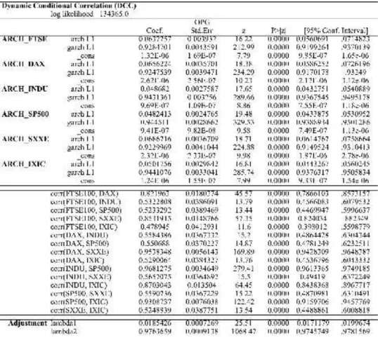
fol-lowing, table 5 shows the DCC estimation with GARCH(1) and ARCH(1).
As table 5 shows, all estimated conditional quasi-correlations are high and
posi-tive between the volatilities of the 6 different indices. For instance, the estimated
condi-tional correlation between INDU and IXIC is 0.8703. This means that high volatility in
the INDU is related to a high volatility in the IXIC and vice versa. The dynamic
condi-tional correlations within the American indices are between 0.87 and 9.97. The
Europe-an estimated correlations have in contrast to the AmericEurope-an indices a little smaller
inter-val, between 0.82 and 0.95. Finally, table 5 presents the results for the adjustment
pa-rameters �
! and �!. Both estimated values for �! and �! are statistically significant. The
estimations for the CCC as well the VCC can be found in Appendix, table 6 and table 7.
The same methodologies of the DCC, CCC and VCC are used for the specific
time frame of the DotCom, which is illustrated in the tables 8, 9 and 10. If �! =�! =0,
than the DCC model reduces the CCC model. Table 11 (and Table 12 for the DotCom
time frame) shows the result of the Wald test - see Wald (1943) - with the null
hypothe-sis that �! =�! = 0 at all conventional levels. The result below indicates that the
as-sumption of constant (time invariant) conditional correlations supposed by the CCC
model is too restrictive for the data set of 6 indices.
TABLE 11. WALD TEST
An interesting finding can be even seen in table 13, 14 and 15. Those tables
in-dicate the different conditional correlation matrix and compared them with the null
hy-pothesis that the correlation between different stock markets is lower during a bubble
means, that the null hypothesis is right and is not rejected. Meaning that during the
DotCom the correlation between the different indices were lower than in the time
with-out bubble. “No” indicates that the conditional correlation is higher during the DotCom.
Table 13 indicates the different conditional correlation in two different time frames. As
one can see, every conditional correlation is higher in the full sample as in the DotCom
time frame. The findings from the conditional correlation of the CCC and the VCC
models confirm this result as well.
TABLE 13. DYNAMIC CONDITIONAL CORRELATION- SAMPLE VS DOTCOM
Figure 9 visualizes the computed individually DCC plots for pair-wise countries
with the different contagion source countries.
The break-point dates are represented by vertical dash circles, which indicate the two
main crises, DotCom (1999-2001) as well the Subprime Crisis (2006-2007). An
inter-esting outcome is that it seems - even with a general high correlation among the
contin-gents - that during a bubble or crisis the contagion decreases. Having a closer look to
the DotCom bubble time, another graphs are plotted, can be seen in figure 9. The time
FIGURE 9. ESTIMATED DYNAMIC CORRELATION COEFFICIENTS
Having estimated the DCC model, the conditional variance is forecasted for the
next 50 time periods into the future. Figure 10 shows the result of those forecasts. From
those conditional variances one can see the impact of crisis to the different stock
mar-kets. As figure 11 illustrates that the variance in period of the DotCom bubble persist
crisis there was an even higher variance. Getting as well a deeper look to the DotCom
bubble, figure 12 illustrates this specific time frame.
6 SUMMARY & CONCLUSION
Given the main objective of this paper to analyze the phenomenon of financial
contagion between stock market returns of different continents, the empirical analysis in
this paper examined the co-movements and spillover effects in the stock market returns
of American and European markets between 1990 and 2014. Three multivariate
condi-tional correlation volatility models were used: the DCC-GARCH by Engle and
Shep-pard (2001), the CCC by Bollerslev (1990) and the VCC by Tse and Tsui (2002).
Throughout the work these methodologies were applied to daily returns of SP500,
INDU and IXIC (all United States), FTSE100 (UK), DAX (Germany) and SXXE
(Eu-rope) for the period from 12/01/1990 to 01/01/2015 and confronted with other models
most widespread in the literature on the subject. The result does not reject the
hypothe-sis of higher contagion in American and European stock markets during crihypothe-sis.
Especial-ly, during the DotCom bubble there was contagion, but not that significant as observed
for the full time sample. All three contagion tests show that multivariate estimates were
significant for all returns in those models and therefore, demonstrate that there have
been changes in the structure of dependence between American and European markets.
This can be caused by different facts, like micro- and macroeconomic factors or even
investors’ behavior. Without any doubt, those impacts can distort the efficient allocation
of investment portfolios and should take into consideration regarding the diversification
analysis. Especially regarding the DotCom bubble, amplifying losses arising from the
negative shocks triggered by the extreme optimism about the new technology industry,
the Internet. Those typical human behavior occurs because the structure of those
wheth-er on a macroeconomic or company scale, by agents - rational and irrational - with the
power to influence the behavior of an entire market, as discussed in Sector 3.4.
The statistical significance of DCC-estimations indicates that the conditional
correlations were dynamic. In fact, the variance-covariance analysis produced useful
information on the dynamic correlations between the three developed markets, and for
each pairwise series, the dynamic conditional correlations vary considerably from their
respective constant correlations, implying the absence of any constant correlation
be-tween the stock markets under study.
The empirical findings showed that the American and European (as well separately
U.K. and German) markets were highly correlated since the end of 1995 with the
begin-ning of the DotCom bubble. These results confirm the presence of spillover effects
7 REFERENCES
Abreu, Dilip and Markus K. Brunnermeier. 2003. “Bubbles and Crashes.”
Econo-metrica, 71: 173204.
Aielli, Gian P. 2013. “Dynamic Conditional Correlations: On Properties and
Estima-tion.” Journal of Business & Economic Statistics, 31 (3): 282–299.
Akaike, Htrotugu. 1973. “Maximum likelihood identification of Gaussian
autoregres-sive moving average models.” Biometrika, 60(2): 255–265.
Akaike, Htrotugu. 1974. “A New Look at the Statistical Model Identification.” IEEE
Transactions and Control, AC-19: 716–723.
Anderson, Keith P., Chris Brooks and Apostolos Katsaris. 2010. “Speculative
bub-bles in the S&P 500: Was the tech bubble confined to the tech sector?” Journal of
Empirical Finance, 17(3): 345–61.
Armada, Manuel J. R., Joao Leitao, and Julio Lobao. 2011. “The contagion effects
of financial crisis on stock markets: What can we learn from a cointegrated vector
autoregressive approach for developed countries?” Revista Mexicana de
Economıa y Finanzas, 6: 29–53.
Arrow, Kenneth. 1982. “Risk Perception in Psychology and Economics.” Economic
Inquiry, 20(1): 1–9.
Arruda, Bruno P. and Pedro L. Valls Pereira. 2013. “Analysis of the volatility’s
de-pendency structure during the subprime crisis.” Applied Economics, 45(36):
5031–5045.
Aschinger, Gerhard. 1991. “Theorie der spekulativen Blasen.”
Azad, Sohel. 2009. “Efficiency, cointegration and contagion in equity markets:
Evi-dence from China, Japan and South Korea.” Asian Economic Journal, 23(1): 93–
118.
Bae, Kee–Hong, G. Andrew Karolyi and Reneé M. Stulz. 2003. “A New Approach
to Measuring Financial Contagion.” Review of Financial Studies, 16(3): 717–763.
Beirne, John, Guglielmo Maria Caporale, Marianne Schulze-Ghattas, and Nicola
Spagnolo. 2009.“Volatility Spillovers and Contagion from Mature to Emerging
Stock Markets.” ECB Working Paper No. 1113.
Belhoula, Malek and Kamel Naoui. 2011. “Herding and Positive Feedback Trading in
American Stock Market: A Two Co-directional Behavior of Investor.”
Interna-tional Journal of Business and Management, 6(9): 244–252.
Blanchard, Olivier J. and Mark W. Watson. 1982. “Bubbles, Rational Expectations
and Financial Markets.” NBER Working Paper Series 945.
Bollerslev, Tim. 1990. “Modelling the Coherence in Short–Run Nominal Exchange
Rates: A Multivariate Generalized Arch Model.” Review of Economics and
Statis-tics, 72(3): 498–505.
Brunnermeier, Markus K. and Stefan Nagel. 2005. “Hedge Funds and the
Technolo-gy Bubble.” Journal of Finance, 59(8): 2013–2040.
Carlos, Anna, Larry Neal and Kirsten Wandschneider. 2006. “Dissecting the
anat-omy of exchange alley: the dealings of stock jobbers during and after the South
Sea Bubble.” University of Colorado Workingpaper.
Celik, Sibel. 2012. “The more contagion effect on emerging markets: The evidence of
Chiang, Thomas C., Bang Nam Jeon, and Huimin Li. 2007. “Dynamic correlation
analysis of financial contagion: Evidence from Asian markets.” Journal of
Inter-national Money and Finance, 26(7): 1206–1228.
Chittedi, Krishna Reddy. 2015. ”Financial Crisis and Contagion Effects to Indian
Stock Market: 'DCC–GARCH' Analysis.” Global Business Review, 16: 50–60.
Cheung Lillian, Laurence Fung, and Chi–sang Tam. 2008. “Measuring Financial
Market Interdependence and Assessing Possible Contagion Risk in the EMEAP
Region.” Hong Kong Monetary Authority Working paper 0818.
Cho, Jang H., and Ali. M. Parhizgari. 2008. “East Asian financial contagion under
DCC–GARCH.” International Journal of Banking and Finance, 6(1): 17–30.
Darbar, Salim M. and Partha Deb. 1997. "Co–Movements In International Equity
Markets." Journal of Financial Research, 20(3): 305–322.
De Bondt, Werner F.M. 1998. ”Behavioral Economics: A Portrait of the individual
Investor.” European Economic Review, 42(3–5): 831–844.
De Bondt, Werner F.M., and William P. Forbes. 1999. ”Herding in Analyst Earnings
Forecasts: Evidence from the United Kingdom.” European Financial
Manage-ment, 5(2): 143–163.
De Long, J. Bradford, Andrei Shleifer, Lawrence H. Summers and Robert J.
Waldmann. 1990a. ”Noise Trader Risk in Financial Markets.” Journal of
Politi-cal Economy, 98(4): 703–738.
De Long, J. Bradford, Andrei Shleifer, Lawrence H. Summers and Robert J.
Waldmann. 1990b. “Positive Feedback Investment Strategies and Destabilizing
Engle, Robert. F., and Kevin Sheppard. 2001. “Theoretical and Empirical Properties
of Dynamic Conditional Correlation Multivariate Garch.” NBER Working Paper
No. 8554.
Fama, Eugene. 1965. “The Behavior of Stock-Market Prices.”The Journal of Business,
38(1): 34–105.
Fama, Eugene. 1970. “Efficient Capital Markets: A Review of theory and empirical
Work.” Journal of Finance, 25(2): 383–417.
Filleti, Juliana de P., Luiz K. Hotta, and Mauricio Zevallos. 2008. “Analysis of
Con-tagion in Emerging Markets.” Journal of Data Science, 6: 601–626.
Forbes, Kristin J. and Roberto Rigobon. 2002. “No Contagion, Only
Interdepend-ence: Measuring Stock Market Comovements.” Journal of Finance, 57(5): 2223–
2261.
Garber, Peter M. 1990. ”Famous First Bubbles.” Journal of Economics Perspectives,
4(2): 35–54.
Hannan, Edward and Barry G. Quinn. 1979. “The Determination of the Order of an
Autoregression.” Journal of the Royal Statistical Society, 41(2): 190–195.
Hesse, Heiko, Nathaniel Frank, and Brenda González–Hermosillo. 2008.
“Trans-mission of Liquidity Shocks: Evidence from the 2007 Subprime Crisis.“ IMF
Working Paper No. 08/200.
Horta, Paulo, Carlos Medes, and Isabel Vierra. 2008. “Contagion effects of the US
Suprime Crisis on Developed Countries.” CEFAGE-UE Working Paper No. 8.
Jarchow, Hans–Joachim. 1997. “Rationale Wechselkurserwartungen,
Devisen-markteffizienz und spekulative Blasen.“ Wirtschaftswissenschaftliches Studium,
26, 509–516.
Kaminsky, Graciela L., Carmen Reinhart, and Carlos A. Vegh. 2003. “The Unholy
Trinity of Financial Contagion.” NBER Working Paper No. 10061.
Karolyi, G. Andrew and Rene M. Stulz. 1996. “Why Do Markets Move Together? An
Investigation of U.S.–Japan Stock Return Comovements.” Journal of Finance,
51(3): 951–986.
Kazi, Irfan A., Khaled Guesmi, and Olfa Kaabia. 2011. “Contagion Effect of
Finan-cial Crisis on OECD Stock Markets.” Economics Discussion Paper No. 2011–15.
Kenourgios, Dimitris, Aristeidi Samitas, and Nikos Paltalidis. 2011. “Financial
cri-ses and stock market contagion in a multivariate time–vaying asymmetric
frame-work.” J. Int. Financ. Mark. Inst. Money 2011, 21: 92–106.
Keynes, John M. 1935. The General Theory of Employment, Interest, and Money. New
York: Harcourt, Brace & World.
Kindleberger, Charles P. 1978. Economic Response: Comparative Studies in Trade,
Finance, and Growth. Cambridge: Harvard University Press.
Kindleberger, Charles P., and Robert Z. Aliber. 2005. Manias, Panics, and Crashe.
Hoboken: John Wiley & Son.
Koller, Tim, Marc Goedhart, and David Wessels. 2010. Valuation: Measuring and
Kugler, Friedrich, and Horst Hanusch. 1992. “Psychologie des Aktienmarktes in
dynamischer Betrachtung: Entstehung und Zusammenbruch spekulativer Blasen.”
Volkswirtschaftliche Diskussionsreihe No. 77.
Kuper, Gerhard H. and Lestano Lestano. 2007. "Dynamic Conditional Correlation
Analysis of Financial Market Interdependence: An Application to Thailand and
Indonesia." Journal of Asian Economics, 18(4): 670–684.
Luetkepohl, Helmut. 2005. New Introduction to Multiple Time Series Analysis.
Michi-gan: Lutz Kilian.
Marcal, Emerson F., Pedro L. Valls Pereira, Diógenes M. L. Martina and Wilson
T. Nakamuraa. 2011. “Evaluation of contagion or interdependence in the
finan-cial crises of Asia and Latin America, considering the macroeconomic
fundamen-tals.” Applied Economics, 43(19): 2365–2379.
Munoz, Pilar, M. Dolores Márquez, and Helena Chuliá. 2010. “Contagion between
Markets During Financial Crises.“ University of Barcelona Working paper.
Nguyen, Tristan and Alexander Schueßler. 2011. “Behavioral Finance als neues
Erk-laerungsansatz fuer “irrationales” Anlegerverhalten.” Diskussionpaper No. 33.
Naoui, Kamel, Seifallah Khemiri, and Naoufel Liouane. 2010. “Crises and financial
contagion: the subprime crisis.” Journal of Business Studies Quarterly, 2(1): 15–
28.
Ofek, Eli and Matthew Richardson. 2001. “DotCom Mania: The Rise and Fall of
In-ternet Stock Prices.” NBER Working Paper No. 8630.
O'Hara, Maureen. 2008. “Bubbles: Some Perspectives (and Loose Talk) from
Parhizgari , Ali. M., Kroshnan Dandapani, and A.K. Bhattacharya. 1994. “Global
market place and causality.” Global Finance Journal, 5(1): 121–140
Pericolo, Marcello and Massimo Sbracia. 2001. “A primer on financial contagion.”
Bank of Italy Working paper.
Phylaktis, Kate and Lichuan Xia. 2009. “Equity Market Comovement and Contagion:
A Sectoral Perspective.” Financial Management, 2009, 38(2): 381–409.
Ross, Stephen A. 2005. Neoclassical Finance. Princeton, NJ: Princeton University
Presp.
Rosser, J. Barkley, Mariana V. Rosser, and Mauro Gallegatiti. 2012. “A Minsky–
Kindleberger Perspective on the Financial Crisis.” Journal of Economic Issues,
46(2): 449–459.
Scherbina, Anna. 2013. “Asset Price Bubbles: A Selective Survey.” IMF Working
Paper 13/45.
Scherbina, Anna and Bernd Schlusche. 2012. “Asset Bubbles: an Application to
Res-idential Real Estate.” European Financial Management, 18(3): 464–491.
Schwarz, Gidon. 1978. “Estimating the Dimension of a Model.” Annals of Statistics,
6(2): 461–464.
Shiller, Robert J. 2000. “Measuring Bubble Expectations and Investor Confidence.”
Journal of Psychology and Financial Markets, 1(1): 49-60.
Simon, Hebert A. 1979. “Rational Decision Making in Business Organizations.”
Tirole, Jean. 1982. “On the Possibility of Speculation under Rational Expectations.”
Econometrica, 50(5): 1163–1181.
Tse, Yie K. and Albert K. C Tsui. 2002. “A Multivariate Generalized Autoregressive
Conditional Heteroscedasticity Model With Time–Varying Correlations.” Journal
of Business & Economic Statistics, 20(3): 351–362.
Wald, Abraham. 1943. “Tests of Statistical Hypotheses Concerning Several
Parame-ters When the Number of Observations is Large.” Transactions of the American
Mathematical Society, 53 (3): 426–482.
Weil, Henry B. 2010. “Why Markets make Mistakes.” Kybernetes, 39(9/10): 1429–
1451.
Williams, John B. 1938. TheTheory of Investment Value. Cambridge, Harvard
Univer-sity Press.
Xiong, Wei. 2013. “Bubbles, Crises and Heterogeneous Beliefs” NBER Working Paper
No. 18905.
Yiu, Matthew S, Wai–Yip Alex Ho, and Lu Jin. 2010. "Dynamic Correlation
Analy-sis of Financial Spillover to Asian and Latin American Markets in Global
8 APPENDIX
FIGURE 5. ALL STOCK MARKET INDICES
TABLE 6. CONSTANT CONDITIONAL CORRELATION
TABLE 8. DYNAMIC CONDITIONAL CORRELATION DOTCOM
TABLE 10. VARYING CONDITIONAL CORRELATION DOTCOM
TABLE 15. VARYING CONDITIONAL CORRELATION- SAMPLE VS DOTCOM
FIGURE 12. CONDITIONAL VARIANCES OF THE RETURNS DOTCOM