Working
Paper
396
The Brazilian Foreign Exchange
Market through the Microstructure
Perspective
Pedro Barguil Collussi
Pedro L. Valls Pereira
CEQEF - Nº23
WORKING PAPER 396–CEQEF Nº 23•JULHO DE 2015• 1
Os artigos dos Textos para Discussão da Escola de Economia de São Paulo da Fundação Getulio Vargas são de inteira responsabilidade dos autores e não refletem necessariamente a opinião da
FGV-EESP. É permitida a reprodução total ou parcial dos artigos, desde que creditada a fonte.
Escola de Economia de São Paulo da Fundação Getulio Vargas FGV-EESP
The Brazilian Foreign Exchange Market through the
Microstructure Perspective
Pedro Barguil Collussi (Sao Paulo School of Economics - FGV)
Pedro L. Valls Pereira (Sao Paulo School of Economics - FGV and CEQEF - FGV)
Resumo
The objective of this study is to investigate whether the relationship between order ‡ow and the spot exchange rate stems from the fact that the ‡ow aggregates information on dispersed economic fundamentals in the economy. To perform this test, a database that includes all transactions of the commercial and …nancial segments of the Brazilian primary foreign exchange market between January of 1999 and May of 2008 was used. We show that the order ‡ow was partly responsible for variations in in‡ation expectations over the time period and that this relationship did not remain robust, drawing comparisons with other fundamentals such as GDP and Industrial Production.
Key words: Exchange Rate Dynamics, Market Microstructure.
JEL Code: F31, G17
1
Introduction
The traditional model of open macroeconomics based on the asset market has existed for over three decades. Despite its intellectually intuitive appeal, no empirical evidence exists that corroborates the model. In this study, while we assume the existence of uncovered interest rate parity and risk neutrality, the interest rate di¤erential between two countries should be fully o¤set by changes in
the exchange rate. However, in practice, we observe that the carry trade1 is not only lucrative but
presents superior returns to the interest rate di¤erential. In the 1980s, Meese and Rogo¤ (1983) showed that a simple random walk possesses greater predictive power than a variety of models based on macroeconomic fundamentals, and the task of explaining exchange rate determinants remains one of the greatest empirical challenges facing researchers of open macroeconomics.
In the last decade, a new micro-founded approach called the microstructural approach was de-veloped to address this problem. Evans and Lyon’s (2002) study is currently the most representative study in this new line of research, and this article also focuses on this area with a speci…c focus on information structure. The novelty of this approach lies in the fact that three hypotheses of traditional models are relaxed: (i) not all relevant information for exchange rate formation is pub-lic; (ii) heterogeneity between agents (either with respect to the mapping of public information or motivation to operate) a¤ects prices; and (iii) institutional arrangements (e.g. lack of transparency) a¤ect prices. In this analysis, one variable is crucial: order ‡ow. This variable is indicative of selling or buying pressure, that is, it is concerned with negotiated volume with a positive (negative) sign if the order that occurred in the market was a purchase (sale).
The second author acknowledge …nancial support from CNPq and FAPESP. Author for correspondence. E-mail: [email protected].
1Operation in which one borrows in a low interest currency and applies to …nancial instruments with high interest
After con…rming the existence of a statistically signi…cant relationship between order ‡ow and exchange rates for the Brazilian case (a result already established in Wu (2007) and Fernandes (2008)), this article attempts to move the discussion forward by investigating the factors that deter-mine the ‡ow. By conciliating microstructure elements through Macroeconomic Theory and based on the theoretical model developed in Evans and Lyons (2007), this article empirically investigates whether exchange rates respond to order ‡ow according to the latter and thus induce changes in market expectations on future economic fundamentals.
To answer this question, the original basis of Wu (2007) was updated to account for all trans-actions between the business and …nancial sector customers of Brazil’s primary foreign exchange market from January of 1999 to May of 2008. Moreover, high frequency estimates were used for the macroeconomic variables (expectations of …nancial institutions collected daily by the Central Bank), which are derived from current and publicly available information. In turn, a high level of accuracy is ensured on ex-ante market expectations on fundamentals rather than ex-post realisations about the own variables.
The remainder of this article is organised as follows. Section 2 describes the market microstruc-ture approach and reviews past empirical studies focused on the foreign exchange market, which provide the basis for this article. Section 3 provides a brief summary on the characteristics of the Brazilian foreign exchange market. Section 4 describes the database employed, and Section 5 elab-orates on the theoretical model. Section 6 presents the empirical analysis, and Section 7 concludes the study.
2
Market Microstructure
A major challenge faced by empiricists in international economics is the task of relating exchange rate movements to macroeconomic fundamentals such as money supply, economic activity and interest rates. Though theory suggests that exchange rates are determined by such fundamentals, with the publication of Meese and Rogo¤ (1983) it has since been accepted that the exchange rate between two countries with similar in‡ation rates can be approximated by a random walk.
Overall, in traditional macroeconomic models, the exchange rate is equal to the present value minus the fundamentals, as shown below:
st= (1 b)
1
X
i=0
biE[ft+i j t] (1)
wherestrepresents the logarithm of the spot exchange rate,0< b <1represents the discount rate,
t denotes current public information at time t and ft represents macroeconomic fundamentals.
Although intellectually intuitive, these models cannot empirically explain a large fraction of the movements that occur in the exchange rate. Flood and Rose (1995), for example, were “led to conclude that the most critical determinants of the exchange rate volatility are not macroeconomics". Lyons (1991) attempted to …ll this gap by unifying elements of Microstructure Theory, which was initially limited to the Theory of Finance (asset pricing, corporate …nance, etc.) that concerns itself with foreign exchange market analysis.
This literature introduces an alternative line of reasoning to Walrasian auction models, which typically assume perfect competition and free entry, that is, a market without friction. As the central focus of this approach is related to the process in which prices incorporate new information, previous studies are related to agent operators known as market makers, who are operators that are willing to buy and sell assets at pre-established prices.
The di¤erence in prices at which these agents buy or sell a particular asset, known as the bid-ask spread comprises one of the simplest forms of friction that arises from asset trading. In microstructure models, variants of the general speci…cations described below are designed to explain
changes in prices quoted by dealers ( pt) as a function of the order ‡ow received ( xt) and as a
function of the change in net exposure by price setters ( It):
pt=f( xt; It; ) +"t (2)
The order ‡ow is positive (negative) when the counterparty buys (sells) the asset at the price quoted by the dealers. The inventory cost can be understood as the risk attributed to the main-tenance of an unwanted position in custody. To retrieve ideal carrying levels, market makers alter prices to those that they are willing to pay or receive for the purchase or sale of assets to prompt the market to take their position. However, this study does not focus on the relationship between
pt and It.
Another area of concern among microstructure models is related to private information and its in‡uence on prices. Information heterogeneity between agents can be illustrated by the varying operating motivations. Certain agents trade for liquidity purposes, smoothing their intertemporal consumption habits by adjusting their portfolios with no information advantage over other agents.
In contrast, informed traders2 have access to some form of private information. The market
maker does not know, a priori, under which category its counterparty falls. However, these individ-uals know, on average, that because they experience losses when operating with the latter group, it is advantageous to o¤set this loss with pro…ts made in dealings with the …rst group.
The learning processes of dealers are thus critical to the determination of asset prices. The di¤erence between the intertemporal behaviours of informed and uninformed traders lies in the fact that the former will establish positions based on ex-ante beliefs on the fundamentals until ex-post information is revealed. Therefore, the direction of transactions (purchase or sale) and traded volume provide information for market makers, and these individuals update their beliefs based on this information. The existence of dispersed private information within the economy and its transmission through the order ‡ow is the mechanism that explains the positive relationship
between pt and xt3 .
The microstructure approach to the foreign exchange market is based, in short, on two central ideas: (i) only part of the macroeconomic information relevant to the exchange rate is publicly known at a given point in time. The remainder of this information remains dispersed and owned by agents privately. (ii) Because the exchange rate constitutes nothing more than the foreign currency price quoted by dealers in terms of the domestic currency, this rate may only re‡ect information known by dealers. Consequently, the exchange rate will only re‡ect information dispersed in the economy when it is assimilated by the dealers - a process that occurs through negotiation.
It is important to note that the fact that the order ‡ow constitutes a proximate cause for exchange rate movements does not contradict the notion that macroeconomic fundamentals are the
2The concept of an informed trader di¤er from an insider, which generally refers to a corporate o¢cer who has
…duciary obligations to its shareholders. There are no insiders in the foreign exchange market.
3The work of Easley and O’Hara (1987) shows that the adjustment path of prices need not necessarily converge
real cause of such movements. According to Evans and Lyons (2002), this interpretation is quite plausible given that empirical forecasting on the expected value of future fundamentals are fairly inaccurate. Orders, on the other hand, re‡ect bets on future fundamentals that are backed by money.
2.1 Empirical Literature Review: Microstructure Applied to Exchange4
Using data from the interdealer market, Evans and Lyons (2002) successfully explain an astonishing 60% of the variation in the Deutsche Mark/dollar exchange rate primarily through order ‡ow. Furthermore, the study shows that buying pressure for dollars worth $1 billion depreciates the dollar price (according to the Deutsch Mark) by 0.5%. In contrast, Evans and Lyons (2005) analyse the relationship between order ‡ows in the interdealer market, as well as ‡ows in the primary market (end-user/dealer)
Evans and Lyons (2007), who are referenced as a theoretical and empirical basis for this article and who therefore will be discussed extensively in other sections, attempt to analyse the relationship
between macroeconomic fundamentals, order ‡ow and exchange rate dynamics5. Their results show
that the ‡ow exerts signi…cant predictive power over macroeconomic fundamentals in addition to those contained in the exchange rate and in other variables. Moreover, they show that the ability of the order ‡ow to predict future exchange rate ‡uctuations is consistent with its ability to predict market reactions to information ‡ows on macroeconomic variables.
By qualifying the discussion on the relationship between fundamentals and exchange rates, Froot and Ramadorai (2005) identify three lines of reasoning. In the "strong"view of the order ‡ow, the order ‡ow induces exchange rate ‡uctuations due to its ability to aggregate private information, which, when revealed, positively and permanently impacts the exchange rate. In the "weak"view of the order ‡ow, the order ‡ow carries information on deviations in fundamentals rather than the actual values of fundamentals and, therefore, impacts the exchange rate only temporarily. Finally, according to the "solely focused on the fundamentals"view, the ‡ow may respond passively to fundamentals or may simply not contain information on fundamentals or fundamental deviations.
The authors examine the relationship between excess currency return6, transaction ‡ows of
institutional investors and macroeconomic fundamentals (actual exchange rate and actual interest rate di¤erentials) and …nd evidence that the ‡ow helps to predict temporary variations in the interest rate di¤erential, which supports the "weak"view of the ‡ow. Evans and Lyons (2007) justify this result on basis of (i) the choice of the fundamentals; (ii) lack of representativeness in the institutional ‡ow (when viewed exclusively); and, most importantly, (iii) the fact that the order ‡ow is not controlled by fundamental variations but by variations in expectations about fundamentals.
Wu (2007) was the …rst study these processes in relation to the Brazilian foreign exchange market. The author’s database is similar to that used for this article, as can be seen in Section
5, and it includes all domestic primary exchange market transactions between July of 1999 and
June of 2003, aggregated daily by counterparty type: business, …nancial clients and the Central
Bank of Brazil. To identify and control bias that may occur with endogeneity between exchange rate movements and foreign currency demands, the author estimates a structural VAR. The results
show that due to a buying pressure of $1billion, dealers depreciate the exchange rate at 2:7%. At
the same time, a depreciation of1% decreases the …nancial sector buying ‡ow by$111million and
the commercial sector by $46million.
4The empirical literature on the ability to forecast out of sample will be discussed in section 6.2. 5See also Engel e West (2005).
The objective of Fernandes (2008) was to compare the Brazilian cash market to its forward exchange rate market. The empirical results show that the forward market demonstrates tighter
spreads and lower-order ‡ow impact on the exchange rate price: The buy (sell) ‡ow of $1 billion
depreciates (appreciates) forward exchange rates at 0:99% and depreciates the spot exchange rate
at 1:12%. Furthermore, whereas the future dollar rate adjusts the order ‡ow in less than three
minutes, the spot price achieves this result in four to …ve minutes. Finally, the author shows that (i) for the prices of the previous ten minutes, (ii) the order ‡ow of the forward market informs the prompt dollar, but the opposite does not occur. This …nding indicates that the forward market is the locus of the exchange rate formation, and then transmitted by arbitration to the spot market.
Laurini et al. (2008) evaluated various empirical properties of the Brazilian foreign exchange market microstructure. Due to the inability to identify, from the obtained database, completed transactions and hence the order ‡ow, the authors instead focused on the bid-ask spread, which can be understood as the inventory carrying cost and/or the liquidity provisions by dealers. For the sample period, it was found that the incorporation of new information into prices is not immediate, which contradicts the e¢cient market hypothesis and corroborating model developed by Easley and O’Hara (1987).
Another interesting aspect of this study included the use of quantile regressions to address the asymmetric process through which the spread becomes related to the market state, measured from uncertainty (volatility) and liquidity (time between two orders in seconds) variables. Spreads above their equilibrium values showed a high degree of persistence and reacted positively in proportion to the quantile with respect to volatility and liquidity. For spreads below their equilibrium value, an opposite relationship was found, denoting a non-linear relationship of mean reversion in the spreads.
3
The Brazilian Foreign Exchange Market
In Brazil, the exchange for physical is split between the primary and secondary market, a system referred to as the interbank. Another relevant locus for exchange rate formation is the derivatives market of the BM&FBOVESPA (São Paulo Stock Exchange). The primary market operation implies e¤ective inputs or outputs of foreign currency within the country. This is the case for transactions between overseas exporters, importers, investors and recipients of funds, interest-paying borrowers and creditors collecting interest from previous debts, travellers etc. In the secondary market, foreign exchange simply migrates from the assets of one bank to another, and these movements are referred to as interbank transactions.
Only those banks authorised by the Central Bank of Brazil perform operations in the secondary market. As in most countries, Brazil has adopted a decentralised market system with multiple dealers. However, as this could not be fully realised, the system possesses certain particularities in
practise7. If negotiations between banks in the international market take place through electronic
systems, the interbank market is largely mediated by brokers who administer their trading desks and real trading sessions by phone. Given its opacity, the learning process for this market, in the words of operators, involves an even greater focus on what Goodhart (1988) called the reading ability of counterparties’ transactions, as well as issues such as reputation and leadership.
Once negotiated, transactions must undergo compulsorily registration and con…rmation in the electronic information system of the Central Bank of Brazil: the Sisbacen. In the forward exchange market, buy-and-sell transactions are administered directly with the Derivatives Clearinghouse of BM&FBOVESPA, which acts as the central counterparty for buyers and sellers. Participants are
required to deposit a bank guarantee, against which daily rate ‡uctuations are charged or credited and multiplied by the value of the contracts to maintain a minimum margin.
The legislation surrounding the forward market is much less restrictive than that of the cash market. While only banks authorised by the Central Bank of Brazil (BACEN) may carry foreign currency in cash, all institutions, as well as individual investors, can carry future positions provided that conditions imposed by the broker and the BM&FBOVESPA are ful…lled. This institutional arrangement causes several unusual spot market transactions to be transferred to the forward mar-ket, which creates a more ‡uid system and, consequently, making the forward market the main locus of exchange rate formation, as is argued by Garcia and Urban (2004).
Operations with …nancial assets are generally targeted at hedging, arbitrage and speculation. In the case of exchange, the most common operation carried out in this market involves arbitrage between interest rates. The bank obtains overseas money located in countries where the interest rate is low - the United States (or Japan) - sells dollars (or yen) over the interbank market and invests in the Brazilian real over the domestic market. In Brazil, we observed that the carry trade is not only lucrative but provides superior returns than the interest rate di¤erential given that the
Brazilian real has undergone an appreciation process from the pre-electoral crisis of 2002until the
outbreak of the 2008 …nancial crisis. Another common practice in the interbank market involves
arbitrage between the exchange rate traded on the secondary market and the rate o¤ered to the customer on the primary market. When buying foreign currency from its customers, for example, the bank attempts to sell that same position over the secondary market with a degree of arbitrage pro…t.
From a practical perspective, numerous issues that the Brazilian exchange market currently faces or has recently experienced are related to information structures. The introduction of prompt
dollar open outcry trading at the BM&FBOVESPA in February of 2006, which was established
through Brazilian Payment System restructuring in 2002, raised doubts over whether order ‡ow
fragmentation between various markets would a¤ect information e¢ciency. The introduction of the electronic trading later on has generated similar issues. With this development, discussions focused on whether the order book should be open to the public, on whether originating institutions should be identi…ed and on the requirements of appropriate order depth.
4
Theoretical Model
4.1 Intuition
Consider a …rm that is willing to pay interest on a liability contracted in dollars from an international funding organisation. This operation a¤ects the Balance of Payments and, therefore, represents a fundamental that should a¤ect the exchange rate. On the other hand, this fact only becomes public after a delay period, which is revealed as a negative item in the Current Account.
The company shall approach a bank (dealer A) to exchange Brazilian reals for dollars in order to complete this transaction. At this time, the company’s private information was transmitted with some degree of accuracy to dealer A through the buy order ‡ow (positive). In general, in the second step of this transaction, the bank uses either the prompt dollar or forward market interbank market
to buy dollars and reduce its exposure while pro…ting from the spread between markets 8. This
successive order ‡ow continues until the exchange rate has reached a new level of equilibrium.
8The mechanism by which the banks; to avoid a mismatch between their current and desired exchange position;
The asymmetry of the information set between agents allows the order ‡ow between primary customers and the dealer, and later among dealers, to impact prices. This is true because the transmission of private information is the primary factor that causes the selling or buying pressure to impact prices permanently.
4.2 Dealers
The theoretical model follows the framework provided by Evans and Lyons (2007). We consider the
optimal choice of M market makers engaged in the foreign exchange market over two negotiation
rounds. In both phases, the prices traded are publicly observed and valid for any dollar amount. In
the beginning, the dealer sets prices, Sm;tI , at which he is willing to sell (or buy) dollars to (from)
primary customers. The orders from primary customers are only observed by the dealer involved in the negotiation and are con…gured as private sources of information.
In the second phase, the dealers set prices, Sm;tII , at which they are willing to negotiate over
the interdealer market. At this time, dealers also initiate businesses using prices provided by other
market makersSm;tII . The net result of orders received by the market makermat stageI is denoted
by Tm;tI . In the second phase, the orders initiated by the dealer mare denoted by IIm;t , and thoese
that are received are denoted by Tm;tII .
The total value of the orders received byM dealers in roundI is equal to the total order ‡ow
for primary customers, xt. The reasoning behind this process is analogous to the next round of
interdealer trading. The total order values received by the dealers are equal to the total order values that the dealers had initiated.
M
X
m=1
Sm;tI Tm;tI = xt (3)
M
X
m=1
Sm;tII IIm;t =
M
X
m=1
Sm;tII Tm;tII (4)
Each quotation must be simultaneously chosen at the beginning of each round, so that:
Sm;tI =Sm;tII =St=f( Mt ) (5)
where Mt =T
m I
m;t is the common information set of all dealers at the beginning of round I in
period t. The balance possesses three basic characteristics: (i) each dealer quotes the same price in
both rounds; (ii) all dealers provide the same pricing; (iii) all quotations set a common information
function that is available at the beginning of the periodt.
The possibility of parallel trading between multiple counterparties and the fact that the
quota-tion is valid for any foreign currency amount excludes the existence of a quote that di¤ers fromStII
in the second round given that, in this case, dealers would be exposing themselves to arbitrage. The
reasoning behind this process is analogous to roundI. The primary customer is free to choose with
whom they will negotiate, implying that dealers should set the same prices, i.e., Sm;tI =Sm;tI =StI
. Finally, while we require incentive compatibility, i.e., that all dealers wish to participate in the
…rst round, we discard any di¤erence betweenSI
t andStII, because each dealer should use the same
Finally, the prices of the …rst round will be common across all market makers only if they depend
on information that is common to everyone, that is, Mt . This however, does not imply that mt
is equal across all markets makers. A market maker m may possess private information at the
beginning of period t on the future spot exchange rate, that is, Em
t [St+1] 6= Etm[St+1], but he or she cannot use this information to inform quoted exchange rate choices without risking arbitrage loss. The agent instead applies this information in second-round allocation decisions, that is, when
buying or selling dollars according to the quote St.
The spot exchange rate is given by the following basic expression:
st= ln(St) = (1 b)EtM
"1 X
i=0
bi ft+i
#
(6)
where EtM is the expectation conditional in Mt . The precise de…nition of fundamentals and the
speci…c parameter form b depend on the macroeconomic model in question and are not the focus
of this study.
For dealers to agree to buy and sell dollars at the exchange rate that they quote, st should be
valued so that excess expected returns o¤set operation risk, .
EtM[ st+i] +rt+i rbt+i = (7)
in which rt+i brt+i is the interest rate di¤erential and is the risk premium.
Equation (6) shows that the dollar price quoted by dealers in Brazilian reals is equal to the expectation and conditioned to dealers’ common beliefs, which is the present fundamentals value. This feature di¤erentiates this variable from (1). The natural consequence of this formulation is the fact that information on the current and future state of the economy will only a¤ect the exchange rate when and if it results in a review of dealer beliefs.
In rewriting (6), we conclude:
st=EtM[ft] +
b
(1 b)E
M
t [ st+i] (8)
st+1=EtM[ st+i] +"Mt+1=
1 b
b st E
M
t [ft] +"Mt+1 (9)
"Mt+1 (1 b)
1
X
i=0
bi EtM+1[ft+i+1] EtM[ft+i+1] (10)
Equation (8) demonstrates that the evolution of the dealers’ information set can a¤ect the exchange rate through two channels. First, it alters the di¤erence between dealer estimates on
the current fundamentals value and the spot exchange rate, st Etm[ft]. Second, it suggests
the occurrence of new reviews on future fundamentals Em
t+1[ft+i+1] Etm[ft+i+1] fori 0, which contributes to dealer prediction errors on spot exchange rates in the future,"Mt+1 st+1 Etm[st+i].
Therefore, any variable correlated with the arrival of new information that allows market makers to
revise their beliefs on future fundamentals, such as the order ‡ow of periodt, must also be correlated
with exchange rate innovation.
Remember that the order ‡ow received in round I includes private dealer information that is
used by dealers to negotiate with other dealers (that is, when choosing II
II aggregates (although partially) information held by the primary customer, or dealer order ‡ow,
which increases the common information set of period t+ 1, Mt+1 , and thus a¤ects the choice of
st+1.
4.3 Order Flow
Without lost of generality, we will analyse the case of a representative primary customer. With this simpli…cation, we disregard the information di¤erence between primary agents. In notation,
we require that pt = pt = P
t . However, we allow for information heterogeneity between dealers
and customers.
The primary agent receives a private signal, represented by the fundamentals, but the infor-mation contains noise. This form of inforinfor-mation can be obtained through searching in the case of investment funds or through the demand for goods and services in the case of …rms. Based on this signal, the agent will begin a transaction through hedging, speculation or arbitrage to pro…t from an information advantage. The total order ‡ow will, therefore, be related to di¤erences between primary customer and dealer estimates on spot exchange rates in the future.
xt= EtP[st+1] EtM[st+1] (11)
where is a positive constant and EtP is the conditional expectation of primary customer belief
sets. If the primary customers are more optimistic than the market makers onst+1, i.e.,EtP[st+1]>
EtM[st+1], buying pressure will develop ( xt>0).
Starting from a very general characterisation of the fundamentals dynamics given in (12), we can draw a direct connection between these dynamics and the order ‡ow, as shown in (21).
ft+1=A ft+ut+1 (12)
In whichut+1 is a vector of shocks with zero mean. When dealers choose the price of the spot
exchange rate according to (6), we can rewrite this last equation as follows:
st='EtM
h!
ft
i
(13)
where:
!
ft=hft ; fti e'=!i1+b(I bA) 1A!i2
then:
EtP [st+1] EtM[st+1] = ' EtPEtM+1 h!
ft+1 i
EtMEtM+1h!ft+1 i
= ' EtPEtM+1h!ft+1 i
EtMh!ft+1 i
(14)
Suppose that the primary customers in instant t collectively know at least as much about the
economy as the market makers do, that is M
t Pt.
Thus, the right hand side of (14) can be rewritten as ' EtPEtM+1h!ft+1
i
EtPEtMh!ft+1 i
and will depend upon customer perceptions on how market makers revise their beliefs on future economic fundamentals.
When Mt = Pt , the di¤erence between expectations on the future exchange rate spot price will
be null because EtM+1h!f t+1 i
EMt h!f t+1 i
M
t . Alternatively, assume that primary customers collectively possess superior information on a
certain variablevt, i.e., Pt = tM; vt . If dealers review their estimates on!ft+1 using elements of
vt, then certain elements ofEtM+1 h!
ft+1 i
EM
t
h!
ft+1 i
will be estimated based on P
t. Therefore,
the order ‡ow should be correlated with variations in fundamentals estimates. Formally, we have:
EhEh!ft+1j Mt+1 i
j Pt
i
= EhEh!ft+1j Mt+1 i
j Mt ; vt
i
= EhEh!ft+1j Mt+1 i
j Mt
i +B
EM t+1
h! ft+1
i
;vt(vt E vtj
M t (15) where B EM t+1 h! ft+1
i ;vt =
Cov Eh!ft+1 j Mt+1
i
; vt
V ar(vt)
(16)
EtPEtM+1h!ft+1 i
EtMh!ft+1 i
=B
EM t+1
h! ft+1
i
;vt(vt E vtj
M
t (17)
EtPEtM+1h!ft+1 i
EtMh!ft+1 i
= EtPh!ft+1 i
EtMh!ft+1 i (18) B EM t+1 h! ft+1
i
;vt BEPt
h! ft+1
i ;vt B EP t h! ft+1
i ;vt 1 B EP t h! ft+1
i ;vt
(19)
for a given ;which Evans and Lyons (2007) called "pace of information aggregation”. If the dealers
do not add new information at t, EM
t+1 h!
ft+1 i
= EM t
h!
ft+1 i
, or if customers expect dealers not
to be able to incorporate new information during period t, EP
t EtM+1 h!
ft+1 i
EP
t EtM
h!
ft+1 i
=
0, will be null9. If period t is completely revealing in such way that tM+1 = Pt, = 110.
EtM+1h!ft+1 i
EtMh!ft+1 i
will be equal to EtP+1h!ft+1 i
EtMh!ft+1 i
. Finally, in intermediary
cases where the pace of aggregation and the incorporation of new information is slower, 0< <1.
In this case, the order ‡ow and di¤erence between expectations of future spot exchange rates between
primary customers and dealers, EtP [st+1] Etm[st+1]will be given by the following expressions:
5EtP[st+1] =EtP [st+1] EtM[st+1] =' EtP
h!
ft+1 i
EtMh!f t+1 i
(20)
xt= ' EtP
h!
ft+1 i
EtMh!ft+1 i
(21)
The basic reasoning of the model suggests that if primary customers possess more information on the economy than dealers and if dealers can assimilate segments of order ‡ow information at each period, the order ‡ow should partly explain variations in di¤erential predictions (between dealers and primary customers) on economic fundamentals.
9Cov Eh!f
t+1j Mt+1 i
; vt = 0
1 0B
EM t+1
h! ft+1
i
;vt=BEtP
h! ft+1
5
Database
The database provided in this article contributes information on transactions between dealers and end users over the primary exchange market, the Real/dollar spot exchange rate, a collection of control variables and a proxy for agent belief changes on macroeconomic fundamentals.
5.1 Flows
Information on foreign exchange transactions was taken from the information system of the Central
Bank of Brazil, Sisbace11, added at daily intervals and measured in billions of dollars; it is calculated
as the di¤erence between the total value of buy orders and total value of sell orders in US dollars.
These data are advantageous, as they provide 100% coverage of primary market transactions
involving the …nancial and commercial sectors. The series identi…es the counterparty type for each transaction, which allows us to determine whether the behaviour of each agent segment is similar and whether the review process of dealer beliefs di¤ers for each type of end user. As transactions over the primary market capture the primitive exchange needs of the economy, the database allows for an analysis that is better aligned with modern macroeconomic theory.
These data also provide an extensive time window, covering the period from January of1999to
May of2008. Moreover, due to the paperwork involved in negotiations over the primary market, the
use of algorithms to identify originators/initiators of transactions is not required, as transactions are carried out directly.
Criticisms of Laurini et al. (2008) about this database are invalidated by the model shown in the previous section. According to the authors, the delay in the disclosure of such information by the Central Bank of Brazil to market agents would imply that such information would not a¤ect trading. The theoretical model, however, clari…es that trading over the primary market involves private information provided to the dealer and that the relationship between the exchange rate and primary ‡ow will be given by the portion of this information to be transmitted to the entire market
through interdealer negotiation at t.
5.2 Expectations
An explanation is appropriate to clarify the di¤erence between the macroeconomic fundamental and
expectations surrounding it. Assume that fundamental f , occurs during the period , that ends
on day T( ), with a value of fT( ). The disclosure of data regarding fT( ) only occurs in D( ),
after period ends and with a delay of D( ) T( ) days. The expectation q of f appraised on
day tbelonging to period is the expected value offT( ) based on the available information set to
dealers earlier on day t, Mt , i.e.:
qT( )jt=E fT( )j Mt (22)
This expectation speci…cation, which occurs on the condition of information available at t,
ensures that the variable can be assumed to a¤ect the market on dayt. Traditional macroeconomic
1 1It is mandatory to register all exchange transactions carried out in Brazil through the Sisbacen, an information
models, in contrast, use series containing information that is not available to market participants
on dayt. Another advantageous attribute of this approach is concerned with data frequency. While
fundamentals are added on a quarterly (in the case of GDP) or monthly (industrial production and
in‡ation) basis, expectations vary from day to day, which is illustrated in …gure 112 and …gure 2.
Evans and Lyons (2007) develop estimates in real time for expectations on fundamentals based on publicly available information until the date in question. For example, using the disclosed data for the period until the second week of August (which includes in‡ation in July, the second quarter GDP, etc.), the authors build an estimate for U.S. GDP growth in the third quarter. The estimate is recalculated every time an update on the state (public disclosure) of an explanatory variable of U.S. quarterly GDP is provided.
This study adopts a simpler approach. We directly apply market expectations on several macro-economic variables that are updated daily by the Central Bank of Brazil from …nancial institutions. "Currently, the research follows market expectations for di¤erent price indices, GDP and industrial production growth, exchange rates, Special Systems for Settlement and Custody (SELIC) rates, tax variables and foreign sector indicators."13
1 2Only as illustrative, disclosure of the series was arti…cially computed as on the last working day of the reference
period.
We used four sets of expectations disclosed by the Central Bank (Banco Central - BACEN): (i) Monthly in‡ation; (ii) twelve-month ahead in‡ation; (iii) monthly industrial production; and (iv) quarterly GDP. We also measured variations in beliefs on these variables at weekly intervals. When two weeks belong to the same period , the development of beliefs is given by the formula:
qT( )jS(j) qT( )jS(j 1) =EhfT( )j MS(j)i EhfT( )j MS(j 1)i (23)
In whichS(j)denotes the last day of the weekj and MS(j) contains only information known at
the beginning of S(j). In this case, expectation development should only include new information
on the value of f in the current period, fT( ) , which denotes that it will not be correlated with
M
S(j 1) . When weekly variations occur in di¤erent periods, we follow:
qT( +1)jS(j) qT( )jS(j 1) = n
EhfT( +1)j MS(j) i
EhfT( +1) j MS(j 1) io
+nEhfT( +1)j MS(j 1)i EhfT( )j MS(j 1)io (24)
The …rst element on the right side of (24) contains new informationfT( +1)and, therefore, should
not be correlated with MS(j 1). The second element identi…es ex-ante expectations of variations in
f between periods and + 1. This term is a function of MS(j 1) and, therefore, can be correlated
to past belief changes.
5.3 Control Variables
Three standard macroeconomic controls are considered in the literature: the interest rate di¤erential measured by the di¤erence between the SELIC and LIBOR rate in dollars (both in % p.a.) over one month; the country risk premium measured by the EMBI + Brazil and IBovespa. All variables were calculated based on the …nal-day closing value of each period. The series were di¤erentiated using:
dif jurt= ln(selict=libort) ln(selict 1=libort 1)
embit= ln(embit) ln(embit 1)
ibovt= ln(ibovespat) ln(ibovespat 1)
Figura 1: Market Expectations IPCA for the current month and disclosed IPCA (percentage pm): 04/2001 to 04/2008
Tabela 1: Estatísticas Descritivas
Mean Median Minimum Maximum Stand. Dev. Asymmetry Kurtoses Autocorrelation
3= 3=2
2 4= 22 1 2
st 0;0028 0:0021 0;1816 0;4952 0;0712 3;2262 23;2920 0;0430 0;0412
Controls
ibovt 0;0207 0;0207 0;1925 0;2155 0;0808 0;2088 2;8946 0;0902 0;0139 embit 0;0154 0;0284 0;3620 0;4562 0;1413 0;6721 4;1618 0;0174 0;1001 dif jurt 0;0022 0;0153 0;3218 0;3806 0;1007 0;6499 5;6096 0;4848 0;3327 Expectation
prodind 0;0183 0;0000 0;8000 0;7000 0;3007 0;3327 3;3035 0;4036 0;0952
ipca 0;0723 0;0350 0;7500 1;7000 0;2672 2;4893 17;4530 0;5922 0;2516 Order Flow
total 1;6155 0;7809 16:5650 6;1333 3;2485 1;5312 6;8785 0;4732 0;4156
comercial 3;0386 2;3182 10;4410 0;5309 2;4691 0;9876 3;4903 0;6975 0;6910
f inanceiro 1;4231 1;1710 6;3789 11;6440 2;4616 0;3633 5;8053 0;3141 0;1145 Notes: All variables are collected at monthly intervals.
critical value of 5%is0;18438
All the analysed series are leptokurtic14with the exception of the geometric return of IBOVESPA.
This last result was not repeated for the daily series, which produced a sample kurtosis of 22:9
(un-reported result). Whereas exchange rate ‡uctuations and in‡ation expectation exhibited a strong trend of right asymmetry, total and commercial order ‡ows demonstrated a clear left asymmetry pattern.
The autocorrelations are positive and signi…cant for the order ‡ow and for the review proxies of dealer expectations. As is shown in …gure 3 , the trade ‡ow is constantly negative, which indicates selling pressures on foreign currency. This fact depicts a condition of positive balances within the
Trade Balance that was experienced in Brazil during this period. Among the months 113included
in the sample, only two showed a positive ‡ow. In the …nancial segment, the series is more volatile,
but 1 is also signi…cant (other lags are not signi…cant). For this segment, the pressure is opposite,
and thus dollars are being bought.
The autocorrelation of expectation variables by dealers demonstrates that growth projections of industrial production or in‡ation are positively related to their respective lags. This implies that a review of dealer beliefs on a particular variable re‡ects the arrival of new information on that variable. Hence, our proxies allow us to capture variations in perceptions on the state of the economy and not on the economy’s actual evolution.
6
Empirical Analysis
To avoid spurious results, ADF and Philips-Perron unit root tests were performed on variables. The
results presented in the table (2-4) demonstrate that the series of order ‡ow is I(0). On the other
hand, the dollar, embi, difjur and ibovespa series are I(1). These were thus were used to ensure
consistent results. Below, the temporal precedence is tested between the disaggregated order ‡ow and the exchange variation.
As shown in table 5 below, the hypothesis that, exchange rate depreciation does not Granger cause commercial order ‡ows is rejected for all frequencies of aggregation. The null hypothesis that trade and …nancial ‡ows are not mutually Granger caused in daily aggregations,is also rejected. For all other combinations of order ‡ows, including commercial and …nancial order ‡ows and exchange rate depreciation, the null hypothesis of no Granger causality, is not rejected.
1 4Compared to a normal distribution, a leptokurtic distribution has a higher peak (higher probability of events
Tabela 2: Unit Root Tests - Daily Frequency
ADF Phillips-Perron
daily variable nothing constant trend nothing constant trend
frequency commercial 0:052 0:006 0:000 0:000 0:000 0:000
…nancial 0:000 0:000 0:000 0:000 0:000 0:000
total 0:000 0:000 0:000 0:000 0:000 0:000
dollar 0:652 0:096 0:405 0:631 0:093 0:395
1st dif 0:000 0:000 0:000 0;000 0:000 0:000
embi 0:202 0:785 0:598 0:180 0:786 0:638
1st dif 0:000 0:000 0:000 0:000 0:000 0:000
difjur 0:514 0:866 0:975 0:507 0:822 0:961
1st dif 0:000 0:000 0:000 0:000 0:000 0:000
IBOVESPA 0:996 0:876 0;771 0:997 0:885 0:797
1st dif 0:000 0:000 0:000 0:000 0:000 0:000
Note: The null hypothesis of non-stationarity range from the most general test to the most speci…c one, and the most suitable option is highlighted in bold.
The reported values are p-values
Tabela 3: Unit Root Tests - Weekly Frequency
ADF Phillips-Perron
weekly variable nothing constant trend nothing constant trend
frequency commercial 0:082 0:014 0:000 0:0000 0:000 0:000
…nancial 0:000 0:000 0:000 0:000 0:000 0:000
total 0:000 0:000 0:000 0:000 0:000 0:000
dollar 0:661 0:086 0:366 0:621 0:078 0:334
1st dif 0:000 0:000 0:000 0:000 0:000 0:000
embi 0:144 0:767 0:688 0:146 0:760 0:647
1st dif 0:000 0:000 0:000 0:000 0:000 0:000
difjur 0:351 0:633 0:902 0:477 0:736 0:928
1st dif 0:000 0:000 0:000 0:000 0:000 0:000
IBOVESPA 0:997 0:867 0:788 0:997 0:861 0:752
1st dif 0:000 0:000 0:000 0:000 0000 0:000
Note: The null hypothesis of non-stationarity range from the most general test to the most speci…c one, and the most suitable option is highlighted in bold.
Tabela 4: Unit Root Tests - Monthly Frequency
ADF Phillips-Perron
Monthly variable nothing constant trend nothing constant trend
Frequency commercial 0;717 0:731 0:000 0:045 0:000 0:000
…nancial 0:000 0:000 0:000 0:000 0:000 0:000
total 0:000 0:000 0:000 0:000 0:000 0:000
dollar 0:481 0:638 0:916 0:480 0:735 0:954
1st dif 0:000 0:000 0:000 0:000 0:000 0:000
embi 0:193 0:753 0:577 0:203 0:740 0:577
1st dif 0:000 0:000 0:000 0:000 0:000 0:000
difjur 0:311 0:494 0:812 0:431 0:647 0:881
1st dif 0:000 0:000 0:000 0:000 0:000 0:000
IBOVESPA 0:998 0:874 0:813 0:997 0:860 0:813
1st dif 0:000 0:000 0:000 0:000 0:000 0:000
Note: The null hypothesis of non-stationarity range from the most general test to the most speci…c one, and the most suitable option is highlighted in bold.
The reported values are p-values
Tabela 5: Granger Causality Test
Frequency Variable 1 Variable 2 p-value
…nancial depreciation 0:197
depreciation …nancial 0:056
Daily commercial depreciation 0:138
depreciation commercial 0:001
commercial …nancial 0:024
…nancial commercial 0:000
…nancial depreciation 0:926
depreciation …nancial 0:336
Weekly commercial depreciation 0:159
depreciation commercial 0:000
commercial …nancial 0:386
…nancial commercial 0:113
…nancial depreciation 0:665
depreciation …nancial 0:193
Monthly commercial depreciation 0:277
depreciation commercial 0:033
commercial …nancial 0:841
6.1 Correlation Between Flow and Depreciation
In Section 4, we noted that the spot exchange rate quoted by dealers must satisfy EM
t [ st+i] +
rt+i rbt+i = . Combining this equation with identity st+1=EtM[ st+1] +st+1 EtM[st+1]and
to equation (13), we have:
st+1 = st+1 EtM[st+1] + Zt
= ' EtM+1h!ft+1 i
EtMh!f t+1 i
+ Zt (25)
Where Zt = rbt+i rt+i + . The risk premium, , is captured by the return of the stock
market and the country-risk premium as measured by Embi+.
In (25) depreciation rates and control variables can be made explicit to review dealer belief sets on the state of the economy.
There are two channels through which dealer belief sets are updated: (i) public information
announced at the start oft+ 1, that is, before dealers quotest+1; (ii) dispersed private information
contained in the order ‡ow between t and t+ 1 and the latter represents the channel that we are
interested in exploring. Assume thatvt is the vector denoting new information obtained by dealers
from the start of tand t+ 1, i. e., Mt+1=f Mt ; vtg:Hence:
EtM+1h!ft+1 i
EtMh!ft+1 i
=Bft+1;vt(vt E vtj
M
t (26)
Because the order ‡ow is an element of vt. when the order ‡ow follows (21), the depreciation
rate can be rewritten as follows:
st+1= ( xt EtM[ xt]) + Zt+ t (27)
in which ='Bft+1;vt and t comprise the portion of '(E
M t+1
h!
ft+1 i
EtMh!ft+1 i
) that is not
correlated with order ‡ow, xt . As an empirical strategy, we use the order ‡ows of …nancial and
commercial sectors as a proxy for( xt EtM[ xt]), , and the results are presented in table 6 below.
Note that the depreciation rate will be correlated with the order ‡ow not only because primary agent and dealer expectations di¤er with respect to economic fundamentals but also because there is a belief that agents that dealers should assimilate a portion of the information through the order ‡ow. In this context, Evans and Lyons (2007) reported that this correlation provides information on: (i) the existence of dispersed information and (ii) the pace at which this information is aggregated.
Di¤erent interpretations can be drawn from the observations provided in table 6 above. First, despite having the expected sign, we note that none of the coe¢cients of the interest rate di¤erentials are statistically signi…cant, which is was expected given the extensive empirical literature that
examines uncovered parity in interest rates.15
1 5Phenomenon known as forward premium puzzle or uncovered parity puzzle. At a theoretical level, there is no
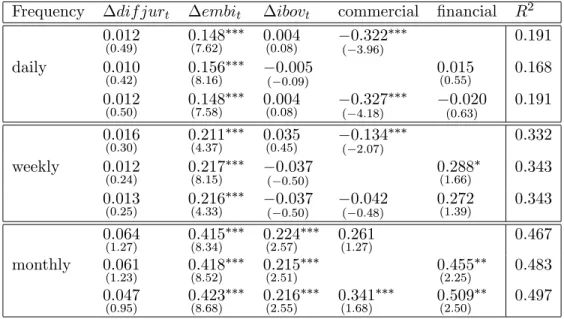
Tabela 6: Order Flow Impact in the Exchange Rate Fluctuation
Frequency dif jurt embit ibovt commercial …nancial R2
0:012
(0:49) 0(7:148:62) 0(0:004:08) ( 30::32296) 0:191
daily 0:010
(0:42) 0(8:156:16) ( 00::00509) 0(0:015:55) 0:168 0:012
(0:50) 0(7:148:58) 0(0:004:08) ( 40::32718) (00::63)020 0:191 0:016
(0:30) 0(4:211:37) 0(0:035:45) ( 20::13407) 0:332
weekly 0:012
(0:24) 0(8:217:15) ( 00::03750) 0(1:288:66) 0:343 0:013
(0:25) 0(4:216:33) ( 00::03750) ( 00::04248) 0(1:272:39) 0:343 0:064
(1:27) 0(8:415:34) 0(2:224:57) 0(1:261:27) 0:467
monthly 0:061
(1:23) 0(8:418:52) 0(2:215:51) 0(2:455:25) 0:483 0:047
(0:95) 0(8:423:68) 0(2:216:55) 0(1:341:68) 0(2:509:50) 0:497 Note: Student t-statistics are listed between parentheses. The order ‡ow
coe¢cients were multiplied by100:Standard errors were corrected through
autocorrelation and heteroskedasticity using Newey-West.
Thus, as was reported in Evans and Lyons (2007), the portion of exchange rate ‡uctuations explained by the variables increases with decreases in the aggregation frequency: the model in
which both primary market segments are addressed where theR2 increases from19%when shifting
from a daily aggregation horizon to one that is weekly, 34% , and …nally to one that is monthly,
50% .]
We now present a technical question. As the coe¢cients of order ‡ows were multiplied by 100,
a buying pressure of $1 billion depreciates the exchange rate in %. It is evident that the order
‡ow impacts within the two segments di¤er considerably. Some impacts are positive, others are negative, and some are statistically signi…cant while others are not. Moreover, it is unclear why the customer order ‡ow apparently contains information on temporal frequency while the other does not.
When aggregation is conducted daily (or weekly for the …rst speci…cation), for example, the coe¢cient measuring the buying pressure impact in the commercial segment is negative and statis-tically signi…cant, which is counterintuitive. According to market makers, a commercial segment buy ‡ow is interpreted as an overvaluing of the dollar. On the other hand, the positive ‡ow from the …nancial sector is positive (that is, the domestic currency is depreciated) in …ve out of six pos-sible scenarios (with the exception of the more complete speci…cation for daily aggregation) and statistically signi…cant in three cases: for the weekly aggregation where only the …nancial ‡ow is considered and for the monthly aggregation for two speci…cations.
The key to interpreting negative coe¢cients that di¤er considerably among themselves lies in
the distinction between non-expected order ‡ow, xt EtM[ xt], as imposed by the model, and the
adopted empirical counterparty, or the primary customer dealer ‡ow. According to the theoretical formulation constructed in this article, the realised exchange rate ‡uctuation re‡ects dealer price reviews, which were induced with the arrival of new information on the state of the economy.
dealer will only a¤ect the exchange rate when it can be inferred through interdealer ‡ows observed by all dealers. Evans and Lyons (2005) show that the coe¢cients of each segment do not o¤er a structural interpretation but, instead, depict how the reviewed set of dealer beliefs in‡uence changes in order ‡ows for each type of end user.
It should be noted that the negative and statistically signi…cant coe¢cient for the commercial sector order ‡ow used in the daily series was also obtained by Wu (2007). According to the author, this phenomenon is caused by endogeneity between the variables, which invalidates the use of the least squares estimation method. On one hand, exchange rate ‡uctuations alter foreign goods and assets prices (as well as perceptions of primary agent impacts on the state of the economy), which a¤ects the order ‡ow; on the other hand, buying pressures on foreign currency contain private information that is perceived by dealers to some degree, which a¤ects the exchange rates that
dealers quote. To enhance the comparative analysis, we estimate structural V ARaccording to the
framework provided by Wu (2007). The results of this analysis are provided in the appendix of this study.
6.2 Out-of Sample Forecast
The purpose of this section is to assess the predictive power of the out-of-sample model. We propose a method that is based on a study by Meese and Rogo¤ (1983). We then identify whether this power is consistent with the capacity for ‡ows to predict fundamentals that a¤ect exchange rates.
Three models will be compared to a random walk (RW) given in (28), which is used as the benchmark. The other models employed include: (i) a pure microstructure model given in (29), in which the explanatory variables comprise order ‡ows from the …nancial and commercial sectors; (ii) a macroeconomic/…nancial model given in (30), which uses the interest rate di¤erential, country-risk premium and Ibovespa as independent variables; (iii) a hybrid model given in (31) that, as developed in this article, incorporates macroeconomic and microstructure elements. The predictive power levels of periods one, two and …ve are compared at several aggregation frequencies (daily, weekly and monthly).
The empirical strategy adopted is the procedure known as rolling regressions, which is commonly
used in the literature.16 This method involves estimating model parameters based on a chosen
sample window (e.g. 100periods) to produce p- out-of-sample forecasts. Subsequently, the sample
window rolls up p-forward periods, and the procedure is repeated. This process is repeated until
all out-of-sample forecasts are generated. This method is advantageous in that the testing power remains constant once the sample window has a …xed size. Models (29), (30) and (31), which are described below, are estimated using the Ordinary Least Squares method.
st+1 st="t+1 (28)
st+1 st= + 1 xcommercial;t+ 2 xf inancial;t+"t+1 (29)
st+1 st= + 3 dif jurt+ 4 embit+ 5 IBOV ESP At+"t+1 (30)
st+1 st= + 1 xcommercial;t+ 2 xf in;t+ 3 dif jurt+ 4 embit+ 5 IBOV ESP At+"t+1 (31)
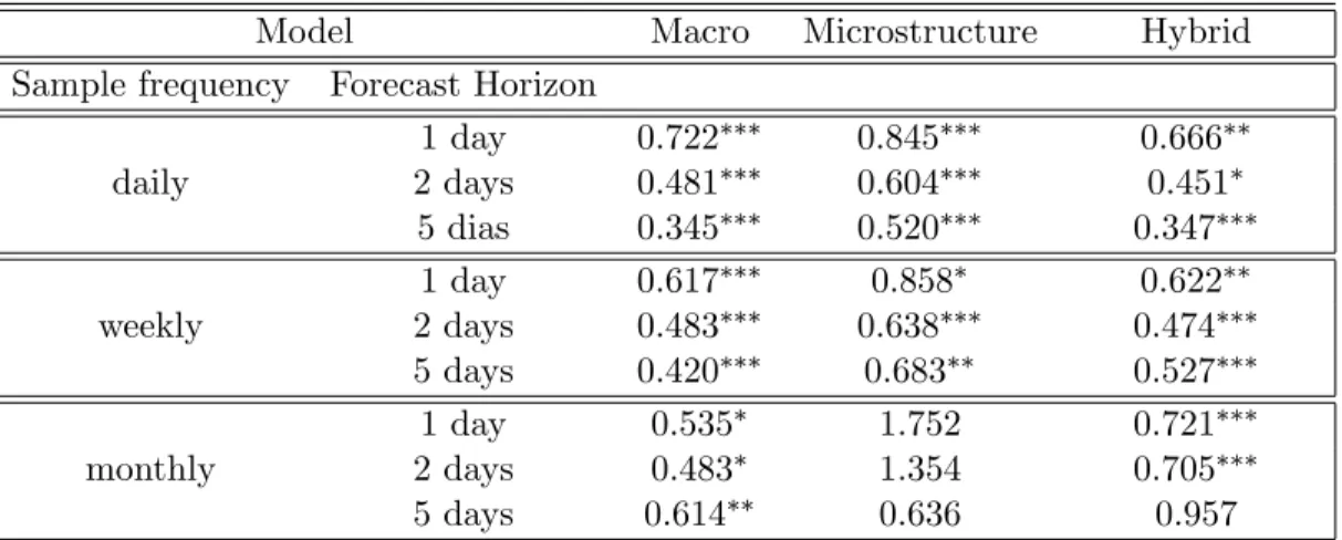
Tabela 7: Mean Squared Error
Model Macro Microstructure Hybrid
Sample frequency Forecast Horizon
1 day 0:722 0:845 0:666
daily 2 days 0:481 0:604 0:451
5 dias 0:345 0:520 0:347
1 day 0:617 0:858 0:622
weekly 2 days 0:483 0:638 0:474
5 days 0:420 0:683 0:527
1 day 0:535 1:752 0:721
monthly 2 days 0:483 1:354 0:705
5 days 0:614 0:636 0:957
Note: Statistical signi…cance of the Diebold-Mariano test is
H0: there is no di¤erentiation in the predictive accuracy of 1%; 5%and 10%
Two metrics will be used to compare the models: (i) the ratio between the Mean Squared
Error of the model in question and random walk –values lower than 1 indicate greater predictive
power (compared to RW) and (ii) a direction change statistic, which denotes the number of correct predictions on the exchange rate change direction over the total number of predictions. (The
prediction reaches the change direction if st+p > 0 occurs simultaneously with bst+p > 0 or
if st+p < 0 occurs simultaneously with sbt+p < 0). For both of these calculations,
Diebold-Mariano statistics, which is de…ned as the ratio between the sample mean of the loss di¤erential and its asymptotic variance, allows us to test the non-di¤erentiation null hypothesis of predictive power (between the model and RW). The di¤erence in loss for the …rst case is calculated as the di¤erence between the model MSE in question and the RW value. In the second case, the di¤erence
in loss, dt takes on a value of1 when the prediction reaches the exchange rate direction of change.
Otherwise, it assumes a null value. Hence, we expect to …nd values ofd higher than50%. In large
samples, the Diebold-Mariano statistic, pd 0;5
0;25=T , follows a normal distribution
17 .
As shown in tables 7 and 8 above, in the frequencies of daily and weekly aggregations for both metrics proposed, the out-of-sample forecast power of the microstructure model is superior to that of the random walk, and this result complements the …ndings of Evans and Lyons (2002) and Fernandes (2008). This result demonstrates that private sources of information are essential for predicting ‡uctuations in exchange rates at high frequencies. Furthermore, we realise that the forecast power of the macroeconomic model is also superior to the RW, which opposes empirical results for pairs of the most heavily traded currencies using high frequency data (Meese and Rogo¤ 1983). As the aggregation frequency is reduced, macroeconomic models can perform more e¤ectively than the RW, as was demonstrated in Chinn and Meredith (2004).
The strong empirical performance of macroeconomic models (compared to RW) is due to the high correlation real/dollar exchange rate ‡uctuations and country-risk premium ‡uctuations, even
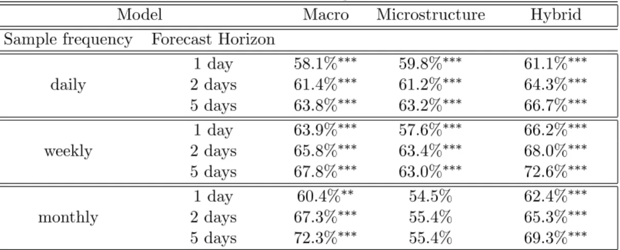
Tabela 8: Variation Change Direction Hit
Model Macro Microstructure Hybrid
Sample frequency Forecast Horizon
1 day 58:1% 59:8% 61:1%
daily 2 days 61:4% 61:2% 64:3%
5 days 63:8% 63:2% 66:7%
1 day 63:9% 57:6% 66:2%
weekly 2 days 65:8% 63:4% 68:0%
5 days 67:8% 63:0% 72:6%
1 day 60:4% 54:5% 62:4%
monthly 2 days 67:3% 55:4% 65:3%
5 days 72:3% 55:4% 69:3%
Note: Statistical signi…cance of the Diebold-Mariano test is
H0: there is no di¤erentiation in the predictive accuracy of 1%; 5%and 10%
in cases where the aggregation frequency is high. According to the Central Bank of Brazil 18,
"variations in perceptions of sovereign risk are generally followed by variations in net capital in-‡ows, which contribute to appreciation or depreciation in the exchange rate". Lowenkron and
Garcia (2005) empirically show that the phenomenon of prime risk19is associated with: (i) currency
mismatch with the government (measured by the ratio between external debt and international reserves) and (ii) low depth of the …nancial market (measured by the ratio between private credit and GDP). When these two factors are latent, an increase in the expected depreciation rate or of the exchange rate risk raises fears surrounding government solvency, which a¤ects perceptions of country-risk. This phenomenon is linked to the inability of certain countries to borrow funds on the international market in their own currencies. This phenomenon was coined as ‘original sin’ by Eichengreen, Hausmann and Panizza (2003).
The hybrid model generates stronger results than the RW for short horizons (daily and weekly). This illustrates the importance of using microstructure elements to capture dispersed private in-formation as a complement to publicly known inin-formation when predicting future exchange rate ‡uctuations.
In practical terms, the capacity for a currency trader to predict the exchange rate change direction of with higher accuracy can be useful for formulating a more lucrative market input rule. As is demonstrated in table 8, the accuracy of the hybrid model increases with a decrease in
aggregation frequency and an increase in the prediction window, which changes from61%to a daily
series with the prediction of one period ahead72;6% in weekly frequency and with the prediction
of 5 periods ahead. This method generates the highest level of accuracy of all of the models.
6.3 Fundamentals
The theoretical model developed in Section 4 shows that if primary customers collectively possess a
set of information that is at least as comprehensive as that of the market makers, that is, Mt Pt
, exchange rate variations should be correlated with order ‡ows because they contain dispersed
1 8http://www4.bcb.gov.br/pec/gci/port/focus/FAQ09-Risco-Pa%C3%ADs.pdf
1 9The positive correlation between foreign exchange rate risk and country risk is known in the literature as “cousin
information on economic fundamentals. If this mechanism drove the results of 6 and 7, the order ‡ow should also explain variations in economic fundamentals. To demonstrate this proposition, we extend the theoretical model by rewriting equation (8) as follows:
st=EtM[ft] +EtM
"1 X
i=0
bi ft+i
#
(32)
It is evident that the di¤erence between the spot exchange rate and current dealer expectations
on economic fundamental values, st EtM[ft], is given by the present value of future changes in
fundamentals.
Empirically, this proposition can be tested using the following projection:
ft+ = s(st EtM[ft]) +"t+ (33)
where "t+ is the projection error that is not correlated with st EtM[ft]. Returning to the
correlation between the order ‡ow and fundamentals, (22), proved that the ‡ow is partly explained by the di¤erence between dealer and end-customer beliefs on future fundamentals. Therefore, if end agents possess a set of information that is superior to dealers, the order ‡ow must o¤er incremental
predictive power over ft+ ,in addition to that contained in st EtM[ft]. In formalising this
reasoning, we show the following:
ft+ = s (st EtM[ft]) + x( xt EtM[ xt]) + t+ 20 (34)
The order ‡ow of periodtwill have incremental predictive power over ft+ when: (i) dispersed
information exists on future economic fundamentals contained therein; (ii) a portion of information
aggregation occurs through negotiation during period t. As st EtM[ft] cannot be measured
directly, we use two known variables at beginning of period t as proxies: qt and st. The
empirical strategy to for analysing this prediction has the following form:
qt+ = + 1 qt+ 2 st+ 3 xcommercial;t+ 4 xf inancial;t+ t+ (35)
where qt = EtM[ft]); qt+ denotes dealer belief reviews on fundamentals accumulated between
periods t and t+ ; qt denotes the review that occurs between instances t and t; st
represents the exchange rate variation value accumulated between t and t; e xj;t, denotes
the order ‡ow for each segment between instances t and t. The empirical counterpart of qt is
the market expectation of various macroeconomic variables, which updated daily by the Central Bank of Brazil from …nancial institutions and which is disclosed through its website and the Focus
newsletter. Coe¢cients 3 and 4 reveal whether the primary customer order ‡ow in instance t
has predictive power over future changes in fundamentals in addition to those contained in the spot exchange rate and in past beliefs. .
2 0Becausev
t E vtj Mt is not correlated to Mt which leads toCov( xt EtM[ xt]; st EMt [ft]) = 0implying