Growth of Brazilian Beef Production:
effect of shocks of supply and demand
Waldemiro Alcântara da Silva Neto1 and Mirian Rumenos Piedade Bacchi2
Abstract: With the considerable growth of beef production in Brazil and the growth in beef exports as a backdrop, the main objective of this study is to identify the factors responsible for the excellent performance of this agribusiness sector. Conducting this study required the construction of a theoretical model that was capable of supporting the specification of the adjusted econometric model using vector autoregression with identification by the Bernanke process. The findings show that the main determinant of beef cattle growth and Brazilian beef exports is increased animal stock. Furthermore, productivity has a positive, albeit more modest, effect on beef production and exports. The results show that the increase of the number of cattle reduces costs to the farmer and retail beef prices.
Key-words: Beef cattle, exports, animal stock, trading.
Resumo: Tendo como pano de fundo o grande crescimento da pecuária de corte no Brasil e o substancial avanço observado nas exportações de carne bovina, este estudo teve como objetivo principal identificar os fatores responsáveis pelo excelente desempenho que vem tendo esse segmento do agronegócio. Para a condução deste trabalho, fez-se necessária a construção de um modelo teórico capaz de dar suporte à especificação do modelo econométrico ajustado utilizando a metodologia de Autorregressão Vetorial com identificação pelo processo de Bernanke. Os resultados obtidos mostram que o principal determinante do crescimento do produto pecuário e das exportações de carne bovina brasileira é o aumento do estoque de animais. Também a produtividade afeta positivamente a produção e as exportações de carne bovina, porém de forma mais modesta. Os resultados indicam que o aumento do rebanho bovino reduz tanto os preços ao produtor como os do varejo de carne bovina.
Palavras-chaves: Pecuária de corte, exportações, estoque de animais, comercialização.
Classificação JEL: Q11, O13.
1. Faculdade de Administração, Ciências Contábeis e Ciências Econômicas, Universidade Federal de Goiás – FACE/UFG. Professor de Economia. E-mail: [email protected]
The general aim of this work is to identify the factors regarding the growth of beef production in Brazil. To achieve this goal, the construction of a theoretical model has been proposed to support the specification of an econometric model that makes it possible to quantify the impacts of variations in the determinants of supply and demand for beef on the volumes of this food that are produced and traded.
Understanding the determinants of growth of beef cattle is very importance for the economy, because it is a key sector for agribusiness GDP and to generate surpluses in the trade balance. The Brazil has the largest commercial herd in the world and is still the largest exporter of beef. It is an activity that requires full attention and facing significant challenges to their growth, which in turn understood, can be the target of public policies.
In the current Brazilian economy, the agribusiness sector has been instrumental in generating income and a balance of trade surplus. Gross Domestic Product (GDP), at the 2012 rate, reached the level of 433.67 billion dollars (Centro de Estudos Avançados em Economia Aplicada – CEPEA, 2013).
Livestock and the upstream and downstream sectors are responsible for approximately one third of the value of Brazilian agribusiness production, and this chain is shown as strategic
value (GPV) of livestock in 2012 was 52.1 billion dollars, while livestock agribusiness (involving the upstream and downstream sectors) had a GPV of 127.9 billion dollars in the same year.
Brazilian livestock has increasingly attracted attention worldwide. Brazil possesses the largest commercial cattle herd, with over 210 million heads of cattle. Since 2004, the country has been the number one world exporter of beef. Furthermore, these exports are destined for a large number of countries, which is desirable from a strategic perspective. In recent decades, the Brazilian frozen foods industry has modernized as well as internationalized. In 2012, the industry slaughtered more than 31 million animals (Brazilian Institute of Geography and Statistics - IBGE, 2013). As a result of these factors cattle-raising is a key industry of the Brazilian economy today, which highlights the importance of academic studies to identify the factors that both drive its growth and might hinder its performance.
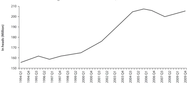
Figure 1. Number of cattle in Brazil, 1994-2009
210
1994 Q1 1994 Q4 1995 Q3 1996 Q2 1997 Q1 1997 Q4 1998 Q3 1999 Q2 2000 Q1 2000 Q4 2001 Q3 2002 Q2 2003 Q1 2003 Q4 2004 Q3 2005 Q2 2006 Q1 2006 Q4 2007 Q3 2008 Q2 2009 Q1 2009 Q4
200
190
180
In heads (M
illion)
170
160
150
Source: IBGE (2010).
the animal slaughtered at an earlier age) are not only desirable for the producer, but also result in lower prices for the consumer.
It is within this context that this study was conducted. Understanding the factors responsible for the growth of Brazilian beef production and exports is, imperative to design appropriate sustainability policies for agribusiness.
The article is organized into five sections. Following the introduction, the second section lays out a brief panorama of livestock production in Brazil. The third section reviews the literature regarding livestock and the theoretical models that address economic growth in various sectors of the Brazilian economy based in the model of Blanchard & Quah. The fourth section presents the proposed model, while the fifth section discusses the results. Lastly, the conclusion lays out final considerations.
2. A brief analysis of
Brazilian beef production
Along with the growth in Brazilian beef production in recent years there has been a considerable increase in exports. Brazil consolidated its position as the country with the
highest number of commercial cattle and the largest beef exporter. The clear increase in the number of Brazilian cattle, including cattle for both beef and milk, can be seen in Figure 1. The data shows that from 1994 to 2009, the number of heads of cattle rose from approximately 155,000,000 to 200,000,000. Looking at it over a longer period of time, from 1945 to 2009, the annual growth rate of Brazilian cattle was 2.37%.
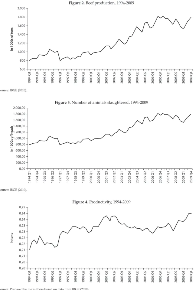
The growing number of cattle resulted in an increase in the number of animals slaughtered and increased beef production (see Figures 2 and 3, respectively). Although the growth of these two factors may appear to be very similar from 1994 to 2009, the growth in meat production was higher than the number of animals slaughtered. This resulted from heavier carcasses, the average weight of which rose from 0.21 to 0.24 tons during those years (Figure 4).
Figure 2. Beef production, 1994-2009 2.000
1994 Q1 1994 Q4 1995 Q3 1996 Q2 1997 Q1 1997 Q4 1998 Q3 1999 Q2 2000 Q1 2000 Q4 2001 Q3 2002 Q2 2003 Q1 2003 Q4 2004 Q3 2005 Q2 2006 Q1 2006 Q4 2007 Q3 2008 Q2 2009 Q1 2009 Q4 1.800
1.400 1.600
1.200
In 1000s of t
ons
1.000 800 600
Source: IBGE (2010).
Figure 3. Number of animals slaughtered, 1994-2009
2.000,00
1994 Q1 1994 Q4 1995 Q3 1996 Q2 1997 Q1 1997 Q4 1998 Q3 1999 Q2 2000 Q1 2000 Q4 2001 Q3 2002 Q2 2003 Q1 2003 Q4 2004 Q3 2005 Q2 2006 Q1 2006 Q4 2007 Q3 2008 Q2 2009 Q1 2009 Q4 1.800,00
1.400,00 1.600,00
1.200,00
In 1000s of heads
1.000,00
800,00
600,00
400,00
200,00
0,00
Source: IBGE (2010).
Figure 4. Productivity, 1994-2009
0,25
1994 Q1 1994 Q4 1995 Q3 1996 Q2 1997 Q1 1997 Q4 1998 Q3 1999 Q2 2000 Q1 2000 Q4 2001 Q3 2002 Q2 2003 Q1 2003 Q4 2004 Q3 2005 Q2 2006 Q1 2006 Q4 2007 Q3 2008 Q2 2009 Q1 2009 Q4 0,24
0,23 0,24
0,23
In t
ons 0,22 0,22
0,21
0,21
0,20
0,20
Figure 5. Largest worldwide exporters of beef (thousands of tons), 1991-2009
1991 1992 1993 1994 1995 1996 1997 1998 1999 2000 2001 2002 2003 2004 2005 2006 2007 2008 2009 2.000
1.500
In 1000s of t
ons
1.000
500
0
Brazil
USA
Australia
Argentina
India New Zealand
Source: United States Department of Agriculture - USDA (2010).
3. Review of the literature
3.1. Meat Sector
In recent literature, some studies have attempted to explain the growth in the meat industry in Brazil, including beef, chicken, and pork. Brandão et al. (2005) aimed to analyze the growth in Brazilian agriculture after the global shift in 1999. The study hypothesized that the growth in soy production took place on degraded cattle pastures rather than on virgen areas in the Cerrado or Amazonian forest. Regarding the favorable performance of livestock, the authors demonstrated that soy temporarily appropriated degraded pastures and that later these pastures were again used as recuperated pastures. Therefore, the profitablity of the practice increased, compared to converting virgin areas. The authors reached the conclusion that soy production increased because of an ‘internal frontier,’ which led to a significant expansion in the Brazilian cattle herd and beef exports.
Resende Filho et al. (2012) aimed to design systemic equations regarding demand for Brazilian meat, based on the theory of the
consumer. The authors showed that Brazil is not only a global leader in the international market for meat, but that Brazil also possesses an extremely important internal market. The results demonstrated that the demand for meat is inelastic and that all of the cross-sectioned elasticities of meat are positive. Therefore, beef and chicken are necessary goods. Based on these results, the authors concluded that profit increases in Brazil would lead to increased consumption of meat, with the exception of swine products. Furthermore, the authors showed that the changes in beef prices due to cross-sectioned elasticities would implicated changes in chicken and pork markets.
the diversity and complexity of strategies, which can lead to conflicts. The authors therefore arrive at the conclusions that, overall: Negotiations can be inefficient and the judicial mechanisms often do not provide the necessary guarantees to efficiently conduct transactions; informal institutions (of producers or cooperatives) can be an alternative given the perception of risk of the transactions; and that the history of conflict contributes to the perception of risk among rural producers. Consequently, for Brazilian livestock production to achieve its full potential and produce the economic gains for actors involved in production and slaughtering, it is imperative to minimize these market failures and provide efficient guarantees for commercialization as soon as possible.
The following section lays out the theoretic models developed in Brazil to address the agricultural growth due to shocks in supply and demand, based on the model of Blanchard and Quah (1989).
3.2. The model of Blanchard and Quah and applications in Brazil
According to Blanchard and Quah (1989), fluctuations in output can be interpreted in two ways 1) demand shocks, which have a temporary effect on production; and 2) supply shocks, which have a permanent effect on production. Other authors, such as King et al. (1991), Gonzaga et al. (1995), Balsameda et al. (2000), Cover et al. (2002) and Maciel (2006) have used determinants similar to those of Blanchard and Quah in their studies on determinants of macroeconomic approaches.
In Brazil, some analysts used Blanchard and Quah’s (1989) derivations as a foundation to propose models that could analyze the behavior of specific economic sectors, particularly agriculture and agribusiness. The studies with this focus are discussed below:
Barros et al. (2006, 2009) sought to analyze the rapid growth in Brazilian agriculture over the last thirty years. For this purpose, they adapted the model of Blanchard and Quah
(1989) to the farming sector in order to measure the impacts of the behavior of macroeconomic and microeconomic variables on the growth of the sector. Their findings showed that Brazilian agriculture has been following a path of growth deriving mainly on productivity gains (over 50% of the growth in farming production has been accounted for by this variable). It has been estimated that a 10% growth in productivity reduces prices by 1.6% and raises production by 4.8%. It has also been pointed out that a great deal of importance can be attached to exchange rates in terms of agricultural growth: a devaluation of 10% increases farming production by 37% and prices by 20%.
Alves et al. (2008) developed an economic model to analyze the growth of Brazilian cotton production from 1960 to the mid-2000s. The authors used the basic ideas of the model of Blanchard and Quah (1989). Their findings showed that the growth in the area of harvested cotton is strongly marked by an autoregressive process. Furthermore, approximately 30% of the growth in cotton production in Brazil was the result of increased cotton plantations. The price evolution was responsible for approximately 15% of the increase in production. The authors concluded that supply-related factors were more important when it came to explaining the development of the Brazilian cotton culture than demand-related factors.
following the shock, stabilizing at 2% after several quarters. A devaluation of exchange rates pushes up exports of products more than the import of fertilizers. Finally, a growth of 1% in GDP makes an expressive impact on the containment of exports of farm produce: -1.7%.
Satolo and Bacchi (2009) sought to explain the growth in sugarcane production in São Paulo State from 1976 to 2006. The authors took the following supply shifters into account: area of cultivated land and price of raw material (sugarcane). The demand shocks are those that impact domestic income, sugar and ethanol prices and the export of these products. The findings showed that exportation was the variable that was most sensitive to shocks, with greater elasticity than the whole in response to the price variations of raw material (sugarcane) and domestic income. The supply shocks and price shocks had permanent impacts on the production of sugarcane and the demand shocks had temporary effects. The authors concluded that the supply shocks are the most important for explaining fluctuations in sugarcane production.
Barros et al. (2006, 2009), Alves et al. (2006) and Satolo and Bacchi (2009), despite basing their models on Blanchard and Quah (1989), did not consider the restrictions that ensured that the supply shocks should be permanent while the demand shocks were temporary. In all cases, the authors used vector autoregression. Although unlike Blanchard and Quah, they identified the structural model from the reduced form using the method proposed by Bernanke (1986).
4. Proposed economic model
The economic model in the present study is based on those used by Barros et al. (2006, 2009), Alves et al. (2006) and Satolo and Bacchi (2008), adapted to livestock. In this case, the method of Bernanke (1986) was also used to identify the structural model from the reduced form.
The demand for livestock produce, in logarithms, is given as:
Ytd=mt−1−ptv (1)
in whichYd is the livestock produce, m is national income and pv is the retail price of beef.
Supply, in logarithms, may be expressed as:
Yt p
s
t t t
p
η θ
= + + (2)
in which η is animal livestock, θis productivity of the herd (average weight of the carcass) and pp is the price received by farmers.
Subtracting the supply of animals from domestic demand, the result is:
Xt Yt Y s
t d
= − (3)
which is the quantity of produce earmarked for the external market.
The shocks that are irrespective of the variables may be expressed as:
a) Internal income (em):
mt mt et m 1
= − + (4)
b) Prices paid to the farmer (ep) and retail prices (ev):
pt p e
p t p t p 1
= − + (5)
ptv=ptv−1+etv (6)
c) Productivity (eθ): e
t t 1 t
θ =θ + θ
− (7)
d) Total animal stock (eη):
E p e
t t
p t
η = ^ h+ η
(8)
et −et 1=µt
η η
− (9)
in which:
E pt p
p t p
1
= −
^ h (10)
thus: p e t t p t 1
η = + η
− (11)
However, domestic and external price evolution over time is considered to be similar, although there is a period of adjustment between them.
4.1. The growth rate of variables
This section presents the growth rates of the variables included in the model.
Substituting equation (11) in equation (2):
yts pt e p
p
t t t
p
1 θ
= + η+ +
− (12)
Substituting equations (12) and (1) in (3):
Xt pt e p m p
p
t t t
p
t tv
1 θ 1
= + η+ + − −
− −
^ h ^ h (13)
or:
Xt pt e p m p
p
t t t
p
t t
v
1 θ 1
= + η+ + − +
− − (14)
Applying the difference and rearranging, the result is:
X X X p p p p
p p e e m m
t t t t p t p t p t p
tv tv t t t t t t
1 1 2 1
1 θ θ 1 1 1
∆ = − = − + − +
+ − + − + η− η − −
− − − −
− − − −
^ ^ ^
^ ^ ^ ^
h h h
h h h h (15)
and, reparameterizing, with the use of equations (4-7) and equation (9), the growth rate of exports is obtained:
Xt et e e e e
p t t m t v t p t 1 µ
∆ = + θ− + + +
− (16)
The exported quantum is affected negatively by internal income. Increased production, animal stock and price paid to the farmer results in increased production and, consequently, exports. On the other hand, higher retail prices lead to less internal consumption, which also results in increased exports.
To obtain the growth rate of livestock production, the difference is applied in equation (12):
Y Y Y p p
e e p p
ts ts ts t p
t p
t t t t t
p t p
1 1 2
1 θ θ 1 1
∆ = − = − +
+ η− η + − + −
− − −
− − −
^
^ ^ ^
h
h h h (17)
By using the relationships expressed in equations (5, 7 and 9), the growth rate of the supply of livestock production is obtained:
Yt e e e
s t p t t p t 1 µ
∆ = + θ+ +
− (18)
Equation (18) shows that, contemporarily, production is affected by price shocks for the farmer, productivity and by shocks to animal stock.
To obtain the growth rate of demand, the difference in equation (1) is applied:
Ytd Ytd Ytd1 mt 1 mt 2 ptv ptv1
∆ = − − =^ − − −h−^ − −h (19)
Reparameterizing, based on the relationships imposed in equations (4-11), the result is:
Yt e e d t m t v 1
∆ = − − (20)
4.2. Methodological approach and data
The VAR – Vector Auto Regression has often been used to analyze complex relationships between variables in one economic model. The advantage of using VAR over other models that also seek to measure these factors is that VAR has a dynamic focus, allowing one to identify not only the magnitude of unanticipated shocks and the accompanying consequences, but also the gap between these effects and the duration of them.
To use the VAR methodology with identification by the Bernanke procedure (structural VAR), it is necessary to use an economic model that supports the specification of the statistic model. The developed theoretical model is used to set the restrictions to be imposed on the matrix of contemporary relations among the variables. These restrictions are necessary for identifying the model in its structural form from the adjustment of the model in its reduced form (ENDERS, 2004).
Table 1. Matrix of contemporary relations
Y X pv pp m η θ
Y 1 0 0 1 (+) 0 1 (+) 1 (+)
X 0 1 1 (+) 1 (+) 0 1 (+) 1 (+)
pv 0 0 1 0 0 0 0
pp 0 0 1 1 0 0 0
m 0 0 0 0 1 0 0
η 0 0 0 0 0 1 0
θ 0 0 0 0 0 0 1
Source: Research data.
Chart 1. Source of the series that make up the theoretical model, quarterly data: 1994-2009
Variable Treatment Used and Description of Variable Basic Data
Internal Income (m) GDP – basic prices in millions of R$; deflated by
the IGP-DI
Ipea - Instituto de Pesquisa Econômica Aplicada (Institute of Applied Economic Research)
Exports (x) Amount exported in tons MDIC/Secex –Ministry of Development, Industry and Foreign Trade
Animal Stock (η) Number of heads of cattle IBGE - Instituto Brasileiro de Geografia e Estatística (Brazilian Institute
of Geography and Statistics)
Produce (Y) Total volume of beef produced, in tons IBGE - Instituto Brasileiro de Geografia e Estatística (Brazilian Institute
of Geography and Statistics)
Productivity (θ)(1) Median weight of carcass Prepared by authors based on data from IBGE - Instituto Brasileiro de
Geografia e Estatística (Brazilian Institute of Geography and Statistics) Price paid to the
farmer (pp)
Price of the bushel of cattle in São Paulo State, deflated by the IGP-DI
IEA SP - Instituto de Economia Agrícola de São Paulo (São Paulo Institute of Agricultural Economics)
Retail prices (pv) Price per kilo of beef in the city of São Paulo,
deflated by the IGP-DI
IEA SP - Instituto de Economia Agrícola de São Paulo (São Paulo Institute of Agricultural Economics)
(1) This variable was constructed based on the figures provided by IBGE: Weight of carcass / Total slaughter (Cows, Oxen and Calves) – Quarterly Survey of Abate (Pesquisa Trimestral do Abate – IBGE).
Source: Prepared by the authors.
unanticipated shock to any of the variables of the model has an influence on all the others.
Another theoretical matter to look at has to do with the stationarity or non-stationarity of the temporal series used in the model. Non-stationary series due to stochastic tendencies (unit root) become stationary after differentiation (ENDERS, 2004). However, if the series are integrated and co-integrated, there is a need to conciliate long- and short-term relations through the use of error-correction models (MADDALA, 2003).
Unit root tests were performed based on the development of Elliot, Rothenberg and Stock (1996), known as the Dickey-Fuller Generalized Least Square– DF-GLS, recommended for use when the number of observations of the temporal series is small and when there are determinist times that are not observed in the generation of the series. Concerning the choice of the number of discrepancies, a criterion proposed by Ng and Perron (2001), known as the
Modified Akaike’s Information Criterion, was used, as recommended in the literature.
The econometric model for the analysis of beef livestock performance in Brazil was adjusted using vector autoregression with error correction (VEC), since the series were integrated and co-integrated, as will be seen below.
The econometric software used for the tests was Regression Analysis of Time Series – Rats 6.2, complemented by Cointegration Analysis of Time Series – CATS.
4.2.1. Data
Table 2. Estimate for the contemporary relation matrix coefficients of the model explaining the determinants of Brazilian beef performance
Influence
Estimated Coefficient Significance Level
Of On
Price paid to farmer Product -0.063 0.5784
Animal Stock Product -1.0747 0.7093
Productivity Product 0.3601 0.0000
Retail Prices Exports -1.8134 0.0286
Price paid to farmer Exports 0.3992 0.6079
Animal Stock Exports -22.013 0.0510
Productivity Exports 1.1537 0.0001
Source: Research data.
5. Results and discussions
The results of the Dickey-Fuller Generalized Least Square (DF-GLS) unit root tests that are necessary for evaluating the stationarity of the series show that they are all integrated to the order of 1 - I(1) if a significance level of probability of 0.05 is considered. Thus, they become stationary after being differentiated (first-order differences). The results were the same for the models in which the trend was considered and for that in which the constant and the trend were considered. The order of each model was determined by the Modified Akaike’s Information Criterion (MAIC).
The Johansen (1988) test was used to test and estimate the long-term relations between variables, which were shown to be integrated to the same order. Given the multivariate analysis context and the possibility of identifying more than one co-integration vector, this procedure is the recommended one. The results showed the existence of two co-integration vectors.
Bearing these results in mind, the VEC (Vector Autoregression with Error Correction) was used to analyze the determinants of beef livestock performance in Brazil. The results are given below, beginning with those concerning the contemporary relations matrix (Table 1). It is worth remembering that the statistic t,in the use of the VEC, is not as rigorous as that observed in the case of models estimated by Least Squares.
Even so, it was reported and analyzed for each estimated coefficient.
One can see that, contemporarily, productivity positively affects meat production: an impact of 1% on the first variable increases production by approximately 0.4%. As expected, the increased median carcass weight results in higher quality beef for the same number of animals slaughtered.
A positive shock of 1% on the retail price reduces exports by 1.8%. This result, although not in keeping with the defined theoretical model, is perfectly compatible with the idea that higher prices may be linked to the scarcity of the product on the market, which may negatively impact exports. Another explanation for this negative relationship between retail price and beef exports could be that lower prices on the domestic market in comparison with the international market stimulates exports and vice versa. In other words, there is the possibility of there being a motion of arbitration, which is responsible for the equalization of prices on the internal and international markets in the long term.
Figure 6. Function of accumulated responses of livestock produce to the shock in the variables of production, exports, productivity, animal stock, prices to the farmer and to retail and internal income
1 2 3 4 5 6 7 8 9 10 11 12
3,00
9,0
7,0
5,0
3,0
1,0
-1,0
-3,0 2,00
Elasticit
y
Elasticit
y
: P
roduc
t/S
tock
1,00
0,00
-1,00
Product/Exports
Product/Retail price
Product/Product
Product/Income
Product/Productivity
Product/Stock
Product/Price to farmer
Source: Research data.
The impact of productivity on exports is positive: an unanticipated shock of 1% on productivity increases exports by 1.2%.
Figures 6 to 10 show the results of the function of response to a boost. They show the effects of shocks on each variable of the system on all the others. In the case of livestock production, what attracts attention is the effect caused by animal stock. Accumulated over six quarters, elasticity is 7.0, stabilizing at 9.0 in the 12th quarter (scale shown on the right axis) (Figure 6).
An unanticipated shock on productivity is rapidly reflected on produce and the effect tends to disappear in the second quarter (constant accumulated elasticity from this period onwards). All the other effects are small. Thus, the two variables that have a greater effect on produce are animal stock and productivity, with the former being the most important.
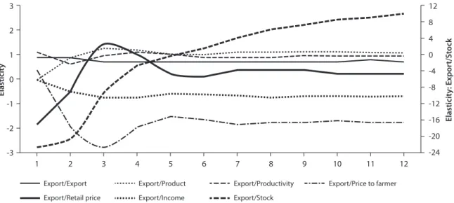
The effects of unanticipated shocks on the variables of the model on Brazilian beef exports are shown in Figure 7. Gains in productivity contemporarily raise the quantity of meat produced, which is reflected in greater surpluses and increased exports. Another expressive effect on exports is produce: it is growing and reaches
a higher accumulated value as early as the third quarter.
The impact of an unanticipated shock on animal stock (scale shown on the left axis) on exports is expressive: a positive shock of 1% on animal stock reduces exports by practically 22% in the first period. Later, the effect becomes positive (after the fifth quarter) and in the twelfth quarter, accumulated elasticity is approximately 10.0.
Retail prices affect exports negatively in the first quarter (approximately -2.0%). As mentioned above, when dealing with results from the contemporary relations matrix, this effect may be linked to the scarcity of the product and the product being directed at the domestic market. Barros et al. (2002), when analyzing the determinants of Brazilian farm produce, found negative elasticity in relation to the domestic price for most of them, with scarcity of the product held responsible. From the third quarter onwards, the effects of retail price on exports are positive. As expected, the effect of income on exports is negative.
Figure 7. Function of accumulated responses of exports to the boost in the variables of production, exports, productivity, stock, prices to the farmer and retail prices and internal income
1 2 3 4 5 6 7 8 9 10 11 12
3 12
-4 0 4 8
-8
-12
-16
-20
-24 2
Elasticit
y
Elasticit
y
: Expor
t/S
tock
1
0
-1
-2
-3
Export/Export
Export/Retail price
Export/Product
Export/Income
Export/Productivity
Export/Stock
Export/Price to farmer
Source: Research data.
Figure 8. Function of accumulated responses of productivity to the boost in the variables production, exports,
productivity, stock, prices to the farmer and retail prices and internal income
1 2 3 4 5 6 7 8 9 10 11 12
3 16
6 11
1
-4 2
Elasticit
y
Elasticit
y
: P
roduc
tivit
y/S
tock
1
0
-1
Productivity/Export
Productivity/Retail price
Productivity/Product
Productivity/Income
Productivity/Productivity
Productivity/Stock
Productivity/Price to farmer
Source: Research data.
to be a predominance of autoregressive behavior by the series. It is important to point out that beef production is often viewed as a “store of value”, with its growth also being due to the expectations of agents in the chain concerning the profitability of other assets, including financial assets.
The responses of productivity to unanticipated shocks on the other variables in
Figure 9. Function of accumulated responses of the price to the farmer from a boost in the variables: production, exports, productivity, stock, prices paid to the farmer and retail and internal income
1 2 3 4 5 6 7 8 9 10 11 12
3 0
-4 -2
-6
-8 2
Elasticit
y
Elasticit
y
: P
ric
e t
o farmer/S
tock
1
0
-1
-2
Price to farmer/Export
Price to farmer/Retail price
Price to farmer/Product
Price to farmer/Income
Price to farmer/Productivity
Price to farmer/Stock
Price to farmer/Price to farmer
Source: Research data.
which have become more commonplace in recent times, in which there is greater control of feeding and the animals gain more weight. When there is a positive shock on retail price, there is a small drop in productivity, which may be linked to increased slaughter, including that of animals with lower weights. Shocks to the other variables of the model have only a small effect on productivity.
An unanticipated shock on animal stock forces the price paid to the farmer up due to lower supply, a trend that is later reversed (Figure 9). As expected, an unanticipated shock in retail price forces the price paid to the farmer down. Barros (1987) explains this as being due to less demand in the retail segment, which makes demand from the farmer and the prices of this segment of the market fall. A positive unanticipated shock on produce results in a slight fall in the price paid to the farmer.
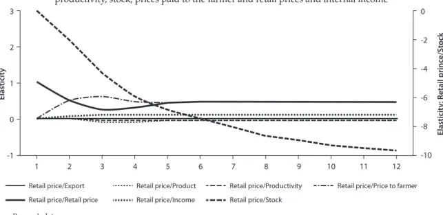
The response of retail price to unanticipated shocks on the other variables of the system is given in Figure 10. An increase of 1% in animal stock reduces retail prices by almost 8% in the second quarter, and this effect persists, reaching an accumulated elasticity of 10.0 in the twelfth quarter (scale shown on the right axis). An unanticipated shock to produce also results in
lower retail prices. However, the accumulated elasticity is small (around -0.7). Impacts of unanticipated shocks on productivity and income are small. An unanticipated shock on price to the farmer increases that of the retail segment.
The historic decomposition of forecast errors enables an analysis of which variables were responsible for the differences between effective values and those forecast within the sample, obtained through the model that captures the median pattern of variation of the series. As the focus of the present study is to analyze production and exports of beef, only the results for these two variables are given.
Figure 10. Function of accumulated responses of retail prices to the boost in the variables: production, exports, productivity, stock, prices paid to the farmer and retail prices and internal income
1 2 3 4 5 6 7 8 9 10 11 12
3 0
-6 -4 -2
-8
-10 2
Elasticit
y
Elasticit
y
: R
etail princ
e/S
tock
1
0
-1
Retail price/Export
Retail price/Retail price
Retail price/Product
Retail price/Income
Retail price/Productivity
Retail price/Stock
Retail price/Price to farmer
Source: Research data.
Figure 11. Production forecasts based on the set of explanatory variables of the model and effective series of beef
production
2000
1994 Q3 1995 Q1 1995 Q3 1996 Q1 1996 Q3 1997 Q1 1997 Q3 1998 Q1 1998 Q3 1999 Q1 1999 Q3 2000 Q1 2000 Q3 2001 Q1 2001 Q3 2002 Q1 2002 Q3 2003 Q1 2003 Q3 2004 Q1 2004 Q3 2005 Q1 2005 Q3 2006 Q1 2006 Q3 2007 Q1 2007 Q3 2008 Q1 2008 Q3
1800
1400 1600
1200
P
roduc
tion (t
on)
1000
800
600
Production
Export + Productivity + Stock + PP + RP + Income
Figure 12. Historical decomposition of total error forecast of beef production in percentages attributed to each variable of the system
0,10
0,05
0,00
-0,05
-0,10
-0,20
F
or
ecast err
or
-0,15
-0,25
-0,30
Total forecast error
Stock forecast error
Product forecast error
PP forecast error
Export forecast error
RP forecast error Income forecast error Productivity forecast error
1994 Q3 1995 Q2 1996 Q1 1996 Q4 1997 Q3 1998 Q2 1999 Q1 1999 Q4 2000 Q3 2001 Q2 2002 Q1 2002 Q4 2003 Q3 2004 Q2 2005 Q1 2005 Q4 2006 Q3 2007 Q2 2008 Q1 2008 Q4
Source: Research data.
Figure 13. Forecast errors for beef production
35%
30%
25%
20%
10%
A
c
cumula
ted f
or
ecast err
ors
Product 15%
5%
0%
2% 5% 9%
12% 16% 19% 22% 26% 29% 33% 36% 40% 43% 47% 50% 53% 57% 60% 64% 67% 71% 74% 78% 81% 84% 88% 91% 95% 98%
Source: Research data.
Analyzing Figure 13, one sees that around 80% of the times the forecast error is under 8%, i.e., 80% of the time, the fundamentals account for at least 92% of the variations in production. The explanatory power of the variables included in the model is considered to be great.
Figure 14 shows that in 1997 and 1998, the most important variable for determining the
Figure 14. Beef export forecasts based on the explanatory set of variables of the model and effective series of beef exports
500.00
1994 Q3 1995 Q2 1996 Q1 1996 Q4 1997 Q3 1998 Q2 1999 Q1 1999 Q4 2000 Q3 2001 Q2 2002 Q1 2002 Q4 2003 Q3 2004 Q2 2005 Q1 2005 Q4 2006 Q3 2007 Q2 2008 Q1 2008 Q4 400.00
300.00
M
ilion (t
on)
200.00
100.00
0.00
Export
Product + Productivity + Stock + PP + RP + Income
Source: Research data.
Figure 15. Historical decomposition of forecast errors of exports in percentages attributed
to each variable of the system
0,80
0,60
0,40
0,20
0,00
-0,40
F
or
ecast err
or
-0,20
-0,60
-0,80
Total forecast error
Stock forecast error
Product forecast error
PP forecast error
Export forecast error
RP forecast error Income forecast error Productivity forecast error
1994 Q3 1995 Q2 1996 Q1 1996 Q4 1997 Q3 1998 Q2 1999 Q1 1999 Q4 2000 Q3 2001 Q2 2002 Q1 2002 Q4 2003 Q3 2004 Q2 2005 Q1 2005 Q4 2006 Q3 2007 Q2 2008 Q1 2008 Q4
Source: Research data.
Based on the information in Figure 16, one can conclude that that 80% of the time the fundamentals account for at least 55% of the variations in Brazilian beef exports. The high values of the observed errors for exports are mainly linked to the huge drop in the international trade of beef in 1997. In the
Figure 16. Forecast errors of Brazilian beef exports
300%
250%
200%
100%
A
ccumula
ted f
or
ecast err
ors
Export 150%
50%
0%
2% 5% 9%
12% 16% 19% 22% 26% 29% 33% 36% 40% 43% 47% 50% 53% 57% 60% 64% 67% 71% 74% 78% 81% 84% 88% 91% 95% 98%
Source: Research data.
6. Conclusions and final considerations
The statistical model used to explain the behavior of Brazilian beef production and exports, adjusted using VEC and Bernake’s identification procedure were shown to be adequate for the aims of this study.
The findings show that animal stock has a positive and considerable impact on produce when the accumulated effects are taken into consideration, although the early impact is negative in both cases. A plausible argument is that in the short term the increase in stock is a result of reduced slaughter, which leads to lower production and fewer exports.
The effect of production on exports is growing and reaches its highest accumulated value in the third quarter. Retail price has a negative effect on exports. Although a higher price may result in lower internal consumption and increased exports, it is necessary to touch on considerations concerning the effect that scarcity of a produce has on prices. Higher prices may be linked to lower availability and, in this case, a fall in exports would be expected. In addition, an arbitration process may account for this negative relationship. Low prices on the internal market in comparison to the international market can
lead to increased exports. In the proposed model, domestic and international prices are considered to have a common trend in the long term, although in the short term there may be disagreements that are corrected through arbitration.
As expected, the effect of income on exports is negative. With higher income, there is more internal consumption and less availability for exports, a relevant aspect of economic growth in Brazil.
Animal stocks do not react very expressively when compared with the impact on the other variables in the model. Indeed, animal stock is expected to be very autoregressive, which is in keeping with the findings of this study. It is important to point out that for a long time, beef production was considered to as a “store of value”, with its growth also being due to expectations by agents in the chain concerning profitability of other activities in the economy.
production is not the same on different farms where cattle are raised, there is clear evidence of greater standardization concerning breeds, resulting in heavier carcasses.
An unanticipated shock on animal stock forces the price paid to the farmer to rise (retention of matrices), which is later reversed. On the other hand, an unanticipated shock on retail forces down the price paid to the farmer. The reason for this is that the fall in consumption in the retail segment, caused by price increases, results in lower demand and a lower price for the farmer.
As expected, an unanticipated shock in produce makes the price to the farmer fall. An unanticipated shock in produce also results in a lower retail price. An unanticipated shock in price to the farmer increases the retail segment.
Concerning the results of historical decomposition of forecast errors (within the sample), the fundamentals (exports, productivity, animal stock, price to the farmer, retail price and income) account for 80% of the times that 92% or more of the variations occurred in livestock produce. In the case of exports, 80% of the times the fundamentals account for under 55% of the variations. Thus, the conclusion is that other variables that are not included in the model may be responsible for the not-so-good adjustment observed in the case of the equation that deals with Brazilian beef exports. Among these variables may be those linked to distinct variations of demand on the international market. A suggestion for future studies could be to explore this subject further.
Other studies can be conducted to look further at environmental matters that permeate the analysis of sustained growth in Brazilian livestock, as the conclusion was reached that the animal stock variable is the most important in explaining the performance of this activity.
7. References
ALVES, L. R. A., BARROS, G. S. A. C. and BACCHI, M. R. P. Produção e exportação de algodão: efeitos de
choques de oferta e de demanda. Revista Brasileira de
Economia, v. 62, n. 4, p. 383-408, 2008.
BALSAMEDA, M., DOLADO, J. J. and LÓPEZ-SALIDO, J. D. The dynamic effects of shocks to labourmarkets:
evidence from OECD countries. Oxford Economic Papers,
n. 52, p. 3-23, 2000.
BARROS, G. S. A. C. Economia da Comercialização
Agrícola. Piracicaba, SP: Fundação de Estudos Agrários Luiz de Queiroz, 1987, 306 p.
BARROS, G. S. A. C., BACCHI, M. R. P. and BURNQUIST,
H. L. Estimação de Equações de Oferta de Exportação de
Produtos Agropecuários para o Brasil (1992/2000). Texto para Discussão. IPEA, n. 865, v. 1-51, 2002.
BARROS, G. S. A. C., SPOLADOR, H. F. S. and BACCHI, M. R. P. Supply and demand shocks and the growth of the brazilian agriculture. In: INTERNACIONAL ASSOCIATION OF AGRICULTURAL ECONOMICS,
Broadbeach. Anais… Broadbeach. IAAE, 2006. No prelo.
______. Supply and demand shocks and the growth of
the brazilian agriculture. Revista Brasileira de Economia,
Rio de Janeiro, v. 63, n. 1, p. 35-50, 2009.
BARROS, G. S. A. C. and SILVA, S. F. A balança comercial
do agronegócio brasileiro de 1989 a 2005. Revista de
Economia e Sociologia Rural, v. 46, n. 4, p. 905-935, 2008.
BERNANKE, B. S. Alternative explanations of
the money-income correlation. Carnegie-Rochester
Conference Series on Public Policy, v. 25, p. 49-100, 1986.
BLANCHARD, O. J. and QUAH, D. The dynamic effects of aggregate demand and supply disturbances.
The American Economic Review, v. 39, n. 4, p. 665-673, 1989.
BRANDÃO, A. S. P., REZENDE, G. C. and MARQUES,
R. W. C. Crescimento Agrícola no Brasil no período
1999-2004: explosão da soja e da pecuária bovina e seu impacto sobre o ambiente. Texto para discussão nº 1103. Instituto de Pesquisa Econômica Aplicada – IPEA, 2005. 22 p.
BRASIL. Ministério do Desenvolvimento, Indústria e Comércio Exterior, 2010. Disponível em: <http:// www.desenvolvimento.gov.br/sitio/interna/interna. php?area=2&menu=885>. Acesso em: 14 abr. 2010.
CALEMAN, S. M. Q. and ZYLBERSZTAJN, D. Falta de garantias e falhas de coordenação: evidências do
sistema agroindustrial da carne bovina. Revista de
Economia e Sociologia Rural, v. 50, n. 2, 2012.
COVER, J. P., ENDERS, W. and HUENG, C. J. Using the aggregate demand-aggregate supply model to identify structural demand-side and supply-side shocks:
results using a bivariate VAR. Working-papers, 2002.
Disponível em: <http://papers.ssrn.com/sol3/papers. cfm?abstract_id=323462>. Acesso: 28 ago. 2009.
ELLIOT, G., ROTHENBERG, T. J. and STOCK, J. H. Efficient tests for an autoregressive unit root.
Econometrica, v. 64, n. 4, p. 813-836, 1996.
ENDERS, W. Applied econometric time series. New York:
John Wiley & Sons, 2004. 466 p.
GONZAGA, G., ISSLER, J. V. and MARONE, G.
Educação, investimentos externos e crescimento econômico: evidencias empíricas. Texto Para Discussão. IPEA, 348, p. 1-28, 1995.
IBGE – Instituto Brasileiro de Geografia e Estatística, 2010. Disponível em: <http://www.ibge.gov.br>. Acesso em: 08 jun. 2010.
IEA – Instituto de Economia Agrícola, 2010. Disponível em: <http://www.iea.sp.gov.br>. Acesso em: 10 jun. 2010.
IPEA – Instituto de Pesquisa Econômica Aplicada, 2010. Disponível em: < http://www.ipeadata.gov.br>. Acesso em: 10 set. 2010.
JOHANSEN, S. Statistical analysis of cointegracion
vectors. Journals of Economic Dynamics and Control, v. 12,
p. 231-254, 1988.
KING, R. G. et al. Stochastic trends and economic
fluctuations. The American Economic Review, v. 81, n. 4,
p. 819-840, 1991.
MACIEL, M. C. Desemprego no Brasil: Evidências da Análise SVAR sob uma Estrutura de Histerese. In: ENCONTRO REGIONAL DE ECONOMIA, 11., 2006,
Fortaleza. Anais... 1 CD-ROM.
MADDALA, G. G. Introdução à econometria. 3. ed. Rio de
Janeiro: LTC, 2003, 345 p.
NG, S. and PERRON, P. Lag Length selection and the construction of unit root tests with good size and
power. Econometrica, v. 69, p. 1519-1554, 2001.
RESENDE FILHO, M. A. et al. Sistema de equações de demanda por carne no Brasil: especificações e estimações.
Revista de Economia e Sociologia Rural, v. 50, n. 1, 2012.
SATOLO, L. F. and BACCHI, M. R. P. Dinâmica econômica das flutuações na produção de
cana-de-açúcar. Economia Aplicada, v. 13, n. 3, p. 377-397, 2009.