A
T
EST
F
OR
S
TRONG
H
YSTERESIS
I
N
I
NTERNATIONAL
T
RADE
V
LADIMIRK
ÜHLT
ELESR
ICARDOD
ENADAIAgosto
de 2009
T
T
e
e
x
x
t
t
o
o
s
s
p
p
a
a
r
r
a
a
D
D
i
i
s
s
c
c
u
u
s
s
s
s
ã
ã
o
o
TEXTO PARA DISCUSSÃO 195 • AGOSTO DE 2009 • 1
Os artigos dos Textos para Discussão da Escola de Economia de São Paulo da Fundação Getulio
Vargas são de inteira responsabilidade dos autores e não refletem necessariamente a opinião da
FGV-EESP. É permitida a reprodução total ou parcial dos artigos, desde que creditada a fonte.
A Test for Strong Hysteresis in International Trade
Vladimir Kühl Teles and Ricardo Denadai FGV-EESP
Abstract
The article suggests a new test for strong hysteresis in international trade. The variables that capture the effects of hysteresis are based on the model of Dixit (1989) with calibrations using a state-space model to determine the parameters for each point in time. These variables are then applied to a cointegration test with breaks, where it is possible to verify whether the hysteresis effect is essential in determining the long-term equilibrium.
Key-Words: Hysteresis, International Trade, Cointegration, Structural Breaks.
1. Introduction
Does economic behavior feature elements of hysteresis? The answer to this question involves the validation of numerous theories regarding international trade, the labor market, and investment. The prescription of public policies in different areas is directly related to this. However, the peculiar nature of behavior in the context of hysteresis remains largely unexplored due to the difficulties in establishing an appropriate econometric testing framework.
This article aims to test strong hysteresis, that is, at the macro level, in the case of international trade. The difficulty in proposing a practical hysteresis test stems from its peculiar nature. A hysteretic economic process retains a memory of past shocks. This
memory is nonlinear and selective, and it exhibits remanence (Hallet and Piscitelli, 2002). As such, a suitable test should be non-linear, as a test of this type selects the shocks that are truly related to hysteresis and verifies whether these temporary shocks are linked with permanent effects.
As explained by Granger and Teräsvirta (1993), there is no test in the econometric time series literature that can take into account all three components of the nature of a hysteresis process. This is because non-linear tests cannot distinguish shocks that are related to
hysteresis from those that are not. In general, tests are used to verify the non-linearity or the remanence of an economic process to determine whether the process is hysteretic.
Efforts to solve this problem are described by Göcke (1994) and Piscitelli et al. (2000), who construct measures of hysteresis and use t tests to verify whether these measures significantly explain a series of behaviors. Their publications offer tests that meet the three defining characteristics of the hysteresis process.
This paper’s contribution is two-fold. First of all, we propose a new measure of hysteresis. Unlike the measures of Göcke (1994) and Piscitelli et al. (2000), our proposed measure is built on a theoretical model. As recommended by Hallet and Piscitelli (2002), the tests proposed by Göcke and Piscitelli et al. might involve variables that are poorly specified or that feature measurement errors. With this in mind, we offer an alternative basis for the analysis in question. Furthermore, by using a theoretical model, we can draw practical conclusions from the actual construction of the suggested measure.
a threshold. When this happens, firms decide to enter the foreign market. Because firms incur sunk costs to begin exporting, they will not stop exporting if the exchange rate falls below this threshold. They will only exit the foreign market if the exchange rate falls below another lower threshold. Therefore, to select which exchange rate shock will hysteretically impact exports, we have to determine the upper and lower thresholds that, in this model, depend on the economy and on Brownian motion parameters governing the exchange rate. Dixit (1994) estimates thresholds for the Japanese economy using a simple calibration of the Brownian motion. Our work extends this approach by using a calibration for each point in time for the parameters and a state-space model to estimate the parameters of Brownian motion at every instant.
Our second contribution is the use of a cointegration test with breaks to verify if the effect of hysteresis is essential to explain the behavior of long-term exports. Our approach is to perform a normal cointegration test without the breaks caused by hysteresis using variables that may determine exports. Then, we repeat the test with the breaks caused by hysteresis dated at the first stage of the test. Thus, in addition to checking the statistical significance of the hysteresis, we observe whether such hysteresis is necessary for the cointegration to occur. In other words, if the variables only cointegrate under the hysteresis effect, we would
conclude that the long-run equilibrium is permanently removed by hysteresis and that without this effect the long-term relationship cannot be explained.
The next section explains the test in detail. Section 3 presents an application to the Brazilian economy, a financial system that has experienced several exchange rate shocks (both apretiation and depreciation) and consequently offers a rich historic background for the analysis in question. The last section offers our final comments.
2. Empirical Methodology
Our first step is to define the inaction zone’s width over time. For this, we use the calibration for the Dixit (1989, 1994) model combined with a state-space model application with
coefficients that vary over time to estimate the Brownian motion of the real exchange rate. This procedure allows us to calculate the evolution of the lower and upper limits of the inaction zone for the period under analysis.
The following section presents the theoretical model of Dixit. After that, we present an overview of our expanded model that includes a state-space framework. Finally, we discuss the test itself.
2.1. The Theoretical Model
The model presented below is a summary of the Dixit (1989) model. This model allows us to determine inaction zone thresholds as originally attempted by Dixit (1994) for the Japanese case.
Consider a company that wishes to enter the foreign market at a cost of K. Once in the market, this company can offer its product at a cost of C reais,1 to generate a return of R US Dollars. The exchange rate is E reais per dollar. Thus, the cash flow yield on sales for this company is given by(ERC), and the company faces a real domestic interest rate of r.
The Brazilian-to-US exchange rate follows a geometric Brownian motion, which is a continuous random path as given by:
dz dt
E
dE
, (1)
where dz is the increment of a standard Wiener process, with no autocorrelation, satisfying 0
) (dz
E andE(dz2)dt
. The expected present value of profit, if the company remains active in the foreign market forever, will beER/(r)C/r. Therefore, the value of an active company, including the value of its option to exit, is:
r C r R E E B E
VA
) ( (2)
When inactive, the company has the option to enter the new market with the value:
A E E
VI( ) (3)
In these expressions, A and B are constants to be determined, and and are the roots of the quadratic equations:
0 ) 1 ( 2 1 )
(x 2x x xr
q
(4)
under the conditions 0and 1 , and over parameters r and, which ensure an appropriate adjustment of values.
Companies’ optimal decision-making will be based on the limit values of the
exchange rate,E and H E , withL EH EL. Any company that has not entered the foreign
market will decide to do so when the exchange rate reaches E , and a company that is active H
in the foreign market will elect to exit it when the exchange rate falls below E . For the L
interval between the two rate limits, the two types of companies maintain their initial decisions.
The value limitsE and H E and the constants A and B are defined by conditions of L
value matching:
K E V E
VI( H) A( H) (5)
VI(EL)VA(EL) (6)
and the conditions of smooth pasting:
) ( ' ) (
' H A H
I E V E
V (7)
) ( ' ) (
' L A L
I E V E
V (8)
The model described achieves some important analytical results, such as elucidating the relationship between hysteresis and the uncertainty related to the foreign market, where an increase in exchange rate uncertainty leads to an increase in the hysteresis effect.
Moreover, it is possible to create numerical simulation exercises based on the model presented. However, the model has to be parameterized, which necessitates solving key equations to obtain the parameters. From (4) it is possible to determine the values ofand, as follows: 2 ] 4 ) 1 [( ) 1
( 2 12
m m
, (9)
2 ] 4 ) 1 [( ) 1
( 2 12
m m
, (10)
where m2/2and2r/2.
At the same time, conditions (5) through (8) can be rewritten using functional forms
follows:
) (
1 C r K
r r
EH
(11) C r r
EL 1 (12) Thus, the model exposes functional forms that are appropriate for numerical
simulations.
2.2. Constructing Hysteresis Thresholds
To calculate the thresholds determined in equations (11) and (12), we must derive values of
their parameters for each point in time. Thus, to obtain σ and the values of μ for each point in
time, we have to estimate a state-space model:
measurement equation
dz dt
E dE
t
, (13)
and transition equation
t t t
t T
1 , (14)
whereE(t)0 eV(t)Qt and the other parameters are obtained through calibration.
Using the model described in the previous section and the parameters obtained, the variables to capture the behavior of hysteresis are defined as follows:
, (13)
where th is determined by the moment when the exchange rate increases above E
H or falls
belowEL for the first time after breaching the other threshold. As an example, let us consider
that the exchange rate falls below EL and then increases and goes beyond EH. In this case, we
have two binary variables with which to define the behavior of hysteresis,1tand 2t, where1t
assumes a value of zero before decreasing to EL and assumes 1 after that, and2t becomes
zero before the rate increases to EH and equals 1 thereafter.
other case t t if h it
0, , 1
2.3. Cointegration Test to Determine Hysteresis
Since we have a hysteresis variable obtained from the theoretical calibrated model as explained in the previous sections, the test of hysteresis essentially consists of verifying whether this variable plays a significant role in determining the long-run equilibrium of trading. To conduct this research, we have to use a cointegration test with structural breaks.
The main goal of this test is to verify whether hysteresis shifts the long-term equilibrium between exports and explanatory variables. Therefore, we must conduct a cointegration test without breaks and a second test with breaks determined by the hysteresis variable. Thus, if cointegration is obtained only by hysteresis-dated breaks, we can say that there is a strong trade-relevant hysteresis effect that shifts the long-term balance.
Several tests of cointegration are currently in use, including the endogenous dating of breaks. Our test follows a similar principle, but break dates are given by the hysteresis variable obtained from the theoretical model.
The cointegration procedure with breaks is proposed by Johansen et al. (2000). The approach suggested is a generalization of the analysis of cointegration based on likelihood in autoregressive vector models as suggested by Johansen (1988, 1996). There are, however, a few conceptual differences, the most significant of which is the need for new asymptotic tables.
3. An Application for the Brazilian case
3.1. Construction and Analysis of Thresholds
3.1.1. Database and Calibration Parameters
The period analyzed extends from January 1992 through December 2006, incorporating several different exchange rate regimes. The data are in the form of 180 observations on a monthly basis.
The series of real effective exchange rates used is calculated by the Brazilian Institute of Applied Economical Research (IPEA). This is a competitiveness measurement of all Brazilian exports, calculated by the weighted average rate of the parity index of purchasing
power across Brazil’s 16 largest trading partners. The parity of purchasing power is defined
National Index of Consumer Prices (INPC / IBGE) of Brazil. The weights used are equal partner with respect to the net sum of Brazilian exports in 2001.
The internal real interest rate is the effective Selic rate accumulated in 12 months and deflated by inflation, measured by the IPCA (IBGE) across a 12-month period. The cost parameters of entering the international market with K = 1 and production cost C = 0.85 (85% of total cost) follow standards presented in the literature (e.g., Dixit 1989, 1994).
3.1.2. Estimating the Equation of the Exchange Rate Brownian Motion
Our first step is to estimate the parameters of equation (13). The parameter was estimated using a time-series model for the real effective exchange rate. We made three estimates for different sampling periods. The first was used for the whole sample. The second took into consideration only the period January 1992 through December 1998. The third estimate focused on the most recent period of the floating exchange regime, starting in January 1999 and ending in December 2006. Our justification for this is that Brazil changed the exchange rate regime, transitioning from a fixed rate to a floating rate, in January 1999, thereby dramatically changing the variance of the exchange rate. Based on these three estimates, we test under two different scenarios. The first uses one value for that is estimated based on data from the entire period, and the second uses different values of for each period.
Table 1: Estimated results for the standard deviation of the real effective exchange rate
Period Sigma
1992:01 to 2006:12 (n = 180) 0.0382
1992:01 to 1998:12 (n = 84) 0.0176
1999:01 to 2006:12 (n = 96) 0.0497
Figure 1. Parameter µ
Therefore, using these variable parameters and a series of monthly internal real interest rates, it is possible to obtain the relevant thresholds over time (equations 9 to 12).
3.1.3. Results and Conclusions
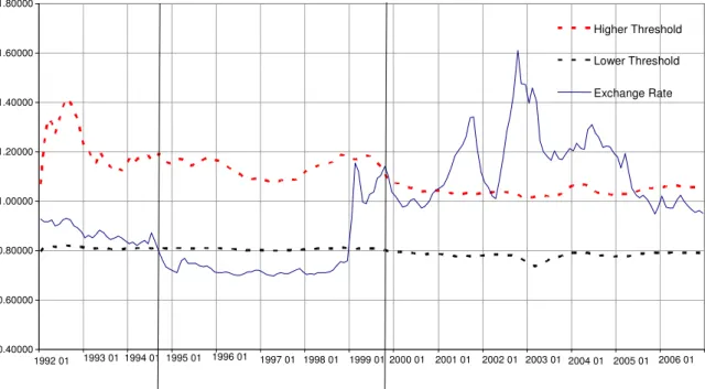
Below, we graph the results for the upper and lower limits of the inaction zone. Our graph also compares the evolution of the real effective exchange rate to the quantum exported.
Case 1.Constant variance throughout the sample period
This exercise considers the variance of the real effective exchange rate to remain constant over the analysis period (this assumption is relaxed below). Despite this, we can draw
Figure 2: Evolution of the Real Effective Exchange Rate (REER) of the Inaction Zone and
the Quantum Exported Thresholds
REER Index: 2000 average = 1 (Source: IPEA).
Quantum index of exports: 1996 average = 100, assuming a 12-month moving average (Source: Funcex).
Parameters: K=1; C=0,85; =0,0382.
The first conclusion relates to the relationship between the behavior of the real effective exchange rate, the limits of the inaction zone, and the quantum exported. There is evidence
0.40000 0.60000 0.80000 1.00000 1.20000 1.40000 1.60000 1.80000
1992 01 1993 011994 011995 01 1996 01 1997 01 1998 01 1999 012000 01 2001 01 2002 01 2003 01 2004 01 2005 01 2006 01
Higher Threshold
Lower Threshold
Exchange Rate
0.40 50.40 100.40 150.40 200.40 250.40 300.40
1992 01 1993 01 1994 01 1995 01 1996 01 1997 01 1998 01 1999 01 2000 01 2001 01 2002 01 2003 01 2004 012005 01 2006 01
Total
that the behavior of quantum exported matches the theory of hysteresis. At the first instant, in September 1994, when the exchange rate falls below the lower limit of the inaction zone, the export quantum drops. It is worth noting that, up to this point, the quantum export trajectory has been rising. At the second time point, beginning in October 1999, when the real effective exchange rate exceeds the upper limit, we observe a significant and consistent increase in the quantum exported for both the total and the manufactured products.
The second important inference relates to the importance of the behavior of the real interest rate in determining thresholds for the inaction zone. In Brazil, we observe a high volatility in the real interest rate, with fluctuations that are of significant magnitude. During the period prior to the Real Plan, the real interest rate ex post accumulated over 12 months reaches 51.4% in August 1992. Even during the period after the implementation of the plan, the country still experiences high real interest rates, even compared with other emerging countries, with periods of high rate volatility due to external shocks. As an example, we cite the peak of 27.4% in October 1998 (the climax of the Russian crisis), just two months before the devaluation of the exchange rate and the change to the exchange rate regime.
Macroeconomic instability and the intensity and volatility of Brazilian interest rates lead to high costs for companies both in terms of financial (i.e., resources and flow capital
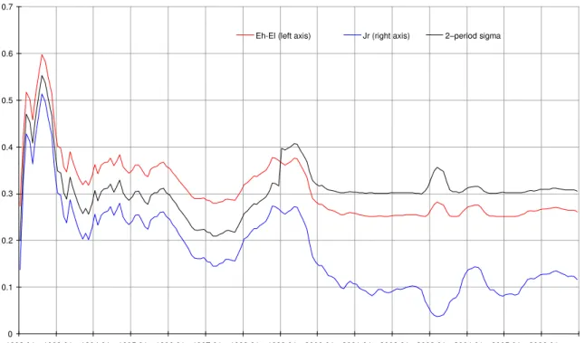
capture) and planning matters (i.e., investment decisions in the long run). Such an impact on Brazilian companies’ decisions to export can be measured by the behavior of relevant inaction zone thresholds. Given the intensity of the interest rate movements, thresholds respond in a significant manner. Figure 3 below illustrates the relationship between the width
of the inaction zone, measured by the difference betweenE andH E , and the behavior of the L
Figure 3: Evolution of the Inaction Zone´s Width and the Real Interest Rate
Figure 3 illustrates the importance of the real interest rate’s evolution over the inaction
zone’s width, even with no changes in exchange rate uncertainty. During the period prior to
the Real Plan (January 1992 to July 1994), we observe a significant increase in this width due to the interest rate shock. The increase in the band’s width significantly intensifies the real exchange rate threshold necessary for Brazilian companies, outside the foreign market, to
decide to export. After the Real Plan, the impact of interest volatility on the band’s width is
clear (due to the external crisis). We note the increase in the interest rate after devaluation (January 1999) and the resulting increase in the zone’s width.
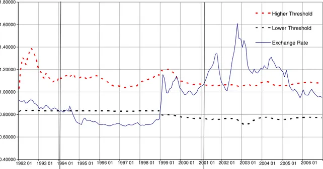
Case 2: Variance for two different sampling periods
In the case of maximum likelihood, we estimate the inaction zone thresholds, taking into consideration the distinct variances of the two periods, namely 1) January 1992 to December 1998, a period remarkable for its fixed exchange rate; and 2) January 1999 to December 2006, a period of flexible exchange rates.
0 0.1 0.2 0.3 0.4 0.5 0.6 0.7
1992 01 1993 01 1994 01 1995 01 1996 01 1997 01 1998 01 1999 01 2000 01 2001 01 2002 01 2003 01 2004 01 2005 01 2006 01 0 0.1 0.2 0.3 0.4 0.5 0.6
Figure 4: Evolution of the Real Effective Exchange Rate (TCRE), including Thresholds of
the Inaction Zone and Quantum Exported
REER Index: average 2000 = 1. Source: IPEA.
Quantum index of exports: average 1996 = 100. 12-month moving average. Source: Funcex.
Parameters K=1; C=0.85; 1=0.0176; 2=0.0497.
Beginning in January of 1994, when the exchange rate falls below the lower limit of the inaction zone, the export quantum declines. When the real effective exchange rate exceeds the upper limit in February 2001, we observe a more pronounced increase in the quantum
0.40000 0.60000 0.80000 1.00000 1.20000 1.40000 1.60000 1.80000
1992 01 1993 01 1994 01 1995 01 1996 01 1997 01 1998 01 1999 01 2000 01 2001 01 2002 01 2003 01 2004 01 2005 01 2006 01
Higher Threshold
Lower Threshold
Exchange Rate
0.40 50.40 100.40 150.40 200.40 250.40 300.40
1992 01 1993 01 1994 01 1995 01 1996 01 1997 01 1998 01 1999 01 2000 012001 01 2002 01 2003 01 2004 01 2005 01 2006 01
Total
exported for the total as well as manufactured products.
Figure 5 illustrates the evolution of the inaction zone’s width over time and shows the
impact of the exchange rate regime change in January 1999. The elevated uncertainty derived from a flexible exchange rate increases the inaction zone’s width. When the change in the exchange rate regime affects the parameters of the stochastic process, which govern the
exchange rate, this in turn determines the parameters of companies’ decisions to enter the foreign market. Therefore, the exchange rate depreciation that is needed in a flexible
exchange rate regime to encourage companies to enter the international market is larger than that associated with a fixed exchange rate regime.
Figure 5: Evolution of the Inaction Zone’s Size and the Real Interest Rate
However, it seems reasonable to assert that gains seen at times of greater economic stability (with controlled inflation and hence lower real interest rates) at least partially offset the increase in uncertainty in relation to the stochastic process that governs the exchange rate in a floating exchange regime. That is, even during the fixed exchange rate period, which allows for greater predictability of exchange rate behavior, the associated high levels and variance of the real interest rate will mitigate the positive effect of greater predictability (lower uncertainty). One only has to observe the behavior of the upper threshold and the
inaction zone’s width.
Macroeconomic stability (control of inflation and consistent reduction of the real interest 0
0.1 0.2 0.3 0.4 0.5 0.6 0.7
rate) allows for a significant reduction of companies’ financial costs, which makes them more competitive. This facilitates a decision to export even in a context of greater exchange rate uncertainty.
Generally, it is clear that another important source of economic policy, also highlighted by Teles (2005), is that excessive exchange rate volatility should be avoided and that it should be stabilized as much as possible in order to reduce the costs (in the form of devaluation) of balancing trade with the foreign sector.
3.2. Testing for Hysteresis
3.2.1. Database and Analysis of Preliminary Data
To estimate equations for exports, we obtained data on the quantum of total exports and manufactured products from the Brazilian Center for the Study of Foreign Trade Foundation (FUNCEX). The division of quantities and values in terms of price is given by the Fisher index, since this takes into account the causes, properties and reversibility of factors—that is, they can be decomposed without severe distortions in indexed quantities and prices, which if recombined return to their original values. Once the price index is obtained, the indexes are implicitly derived from the quantum, obtained by deflating the values exported by the price variations.
The commodities prices (excluding fuels) index calculated by the IMF
(International Monetary Fund) is used as a proxy for Brazilian export prices. The price index base is such that 1995 = 100, which includes the prices of industrial products and those of food and beverages. This index is informally used by the Central Bank of Brazil. The total volume of manufactured product exports is denoted, respectively, by XQTB and XQMB; the real effective exchange rate is given by E, while P is the IMF price index for commodities (excluding fuels).
To capture the effect of income growth in the rest of the world (foreign demand), the deterministic trend term is included in all models. Kannebley (2005) argues that the
deterministic trend term apparently matches the representative demand variable, suggesting that this component in some way reflects the tendency component associated with
international demand.
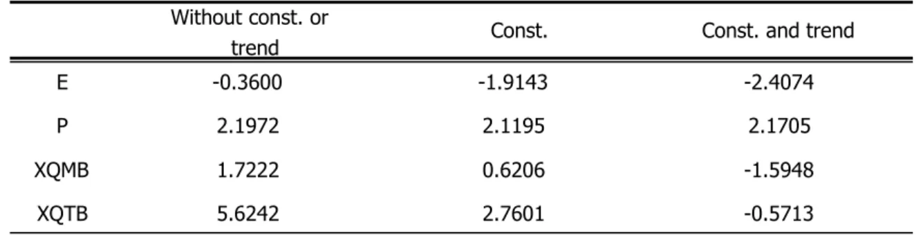
To determine the order of integration of the variables used, we conduct
Table 2: Statistics of the Dickey-Fuller Increased (ADF) Test
The statistics from this table fail to reject the null hypothesis for any level of significance: 1%, 5%, or 10%.
Lags are chosen according to the information criteria from Schwarz.
To be certain of the nonstationarity of these series, the ADF test is complemented by the Kwiatkowski-Phillips-Schmidt-Shin (KPSS) test. Our null hypothesis, in the case of the KPSS test, is the opposite of the ADF test. The null hypothesis confirms whether the series is stationary. We reject the null hypothesis to corroborate the presence of a unit root as
indicated by the previous test. The selection of the number of lags is automatic, according to the Newey-West criteria (using the method of spectral estimation from Bartlett Kernel). The null hypothesis of stationarity is rejected independently of the deterministic terms
specification. In both models (with intercept alone, and with both trend and intercept), the resulting statistics were greater than the critical values for a significance level of 5%, except for the variable P in the case of the one-constant model (which reached a 10% level of significance).
Table 3: Kwiatkowski-Phillips-Schmidt-Shin (KPSS) statistics
Statistical test rejects the null hypothesis of stationarity for: * 1%, ** 5%, *** 10%. Method of spectral estimation: Bartlett Kernel.
Const. Const. and trend
E 1.017793* 0.194545**
P 0.409413*** 0.290041*
XQMB 1.461785* 0.370572*
XQTB 1.558388* 0.404563*
Without const. or
trend Const. Const. and trend
E -0.3600 -1.9143 -2.4074
P 2.1972 2.1195 2.1705
XQMB 1.7222 0.6206 -1.5948
Bandwidth according to the Newey-West criteria.
The nonstationarity of the time series allows us to estimate the cointegration relationship among the variables.
3.2.2. The Brazilian Case
We aim to test the stability of long-term relationship of the volume of Brazilian exports and international commodity prices and the real effective exchange rate. Given that the
explanatory variables are I(1) according to the ADF and KPSS tests, the linear combination may result in a stationary series, which allows the use of a cointegration vector.
3.2.2.1 Johansen Cointegration Test with Structural Break
The model of the Johansen test with a known structural break was previously discussed. We conduct three different tests for the volume of total exports and the volume of manufacturing-relevant exports. The first test is the trace statistic of the Johansen without breaks. We then repeat the test with two breaks (obtained in section 3). The first pair, with breaks in
September 1994 and October 1999, was obtained by assuming constant variance for the entire sample period. The second pair, with breaks in January 1994 and February 2001, were
obtained given the different REER variance across two periods of relevance: before and after the exchange rate devaluation in January 1999. Our method tests two types of breaks: (i) at level (ii) at level and trend.
We chose to use the model with two deterministic terms, namely constant and trend.
Trend represents the growth of the world’s demand for exports due to the increase in worldwide income over time.
For the cointegration test, it is necessary to specify the number of lags of the
autoregressive vector (VAR). We consider a maximum of 15 lags given that we are dealing with monthly data. We use four criteria: Akaike Info Criterion (AIC), Final Prediction Error (FPE), Hannan-Quinn Criterion (HQ), and Schwarz Criterion (SC). The number of lags used was suggested by the largest number of criteria (bold values in Table 4). When each criterion points to a different lag, we use the criteria suggested by Schwarz, since the sample consists of 180 observations.
We also chose to include seasonal dummies in all tests given the nature of the quantum of Brazilian export series. The deterministic term is:
(14)
Seasonal dummies t
The critical values (and p-values) of Johansen’s trace statistics are obtained by computing the response surface according to Doornik (1998) (if no breaks) or according to Johansen et al. (2000) (with up to two breaks). In the case of breaks at level, the response surface also follows Johansen et al. (2000). Next, we present our test results for a 5% significance level.
Table 4: Cointegration Test from Johansen, with and without Breaks for XQTB, E and P
Table 4 presents the results of trace statistics for the total Brazilian exports quantum (XQTB), the real effective exchange rate (E), and the index prices of commodities excluding fuels (P). Zero and one or two cointegration vectors are possible among the three variables. In all cases (with and without structural breaks), the null hypothesis of no cointegration vector (r = 0) is rejected at the expense of the alternative hypothesis (r > 0). As such, the results
suggest a long-term relationship among variables even without breaks. That is, although the variables in the equation are nonstationary, the linear combination is stationary, which implies that they cannot be too distant from each other for an extended period of time.
TERMS LAGS H0 HA Stat. 5% P-Value
r = 0 r > 0 49,61 42,77 0,0081
r = 1 r > 1 20,81 25,73 0,1905
r = 2 r > 2 4,82 12,45 0,6280
r = 0 r > 0 81,44 58,48 0,0001
r = 1 r > 1 40,62 36,85 0,0189
r = 2 r > 2 15,28 18,62 0,1417
r = 0 r > 0 90,82 72,59 0,0009
r = 1 r > 1 40,38 46,75 0,1736
r = 2 r > 2 19,80 24,21 0,1595
r = 0 r > 0 94,58 58,15 0,0000
r = 1 r > 1 36,46 36,55 0,0511
r = 2 r > 2 10,38 18,6 0,4546
r = 0 r > 0 101.25 71.02 0.0000
r = 1 r > 1 41.45 45.64 0.1179
r = 2 r > 2 15.98 23.54 0.3260
AIC: Akaike Info Criterion FPE: Final Prediction Error HQ: Hannan-Quinn Criterion SC: Schwarz Criterion
Level Level and Trend Sep/1994 and Oct/1999 Jan/1994 and Feb/2001 BREAKS No Level Level and Trend Const. and Trend
6 (AIC, FPE); 2 (HQ); 1 (SC)
Const. and Trend
2 (FPE, HQ); 19 (AIC); 1 (SC)
Const and Trend
2 (FPE, HQ); 20 (AIC); 1 (SC)
Const and Trend
1 (SC); 20 (AIC); 6 (FPE); 2 (HQ)
Const and Trend
Table 5: Johansen Test With and Without Breaks for XQMB, E and P
Table 5 presents trace statistics for the total Brazilian exports quantum of
manufactured goods (XQMB), the real effective exchange rate (E) and the index of prices of commodities excluding fuels (P). Zero and one or two cointegration vectors are possible among the three variables. The hypothesis of no cointegration vector cannot be rejected when structural breaks are disregarded. In all cases (with and without structural breaks), the null hypothesis of no cointegration vector (r = 0) is rejected at the expense of the alternative hypothesis (r > 0). As such, our results suggest a long-run equilibrium among variables only if breaks are considered. This suggests the existence of hysteresis in manufacturing exports.
3.2.2.2. Estimation of the Cointegration Vectors
In addition to the cointegration tests, cointegration vectors can provide information about the relationship between structural breaks obtained from the hysteresis theory and the long-run equilibrium of the foreign sector. A total of 11 dummy variables (exogenous) were used to correct for seasonal variations (one for each month of the year plus the constant).
Since our objective is to test for hysteresis in Brazilian foreign trade, we extend our analysis only for the volume of manufactured exports (XQMB), as there is clear evidence of hysteresis in this category.
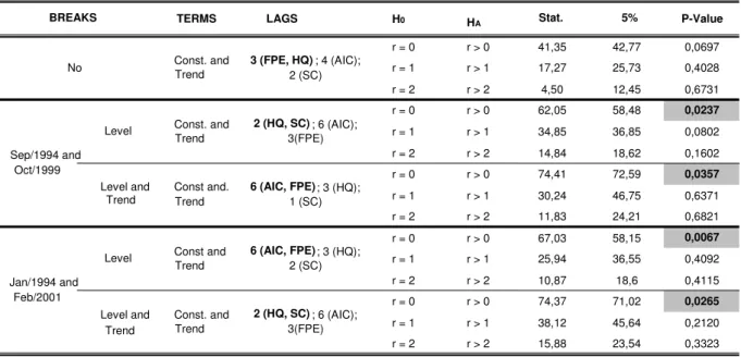
Table 6 shows long-term estimates of cointegration vectors for the models with trend
TERMS LAGS H0 Stat. 5% P-Value
r = 0 r > 0 41,35 42,77 0,0697
r = 1 r > 1 17,27 25,73 0,4028
r = 2 r > 2 4,50 12,45 0,6731
r = 0 r > 0 62,05 58,48 0,0237
r = 1 r > 1 34,85 36,85 0,0802
r = 2 r > 2 14,84 18,62 0,1602
r = 0 r > 0 74,41 72,59 0,0357
r = 1 r > 1 30,24 46,75 0,6371
r = 2 r > 2 11,83 24,21 0,6821
r = 0 r > 0 67,03 58,15 0,0067
r = 1 r > 1 25,94 36,55 0,4092
r = 2 r > 2 10,87 18,6 0,4115
r = 0 r > 0 74,37 71,02 0,0265
r = 1 r > 1 38,12 45,64 0,2120
r = 2 r > 2 15,88 23,54 0,3323
AIC: Akaike Info Criterion FPE: Final Prediction Error HQ: Hannan-Quinn Criterion SC: Schwarz Criterion
BREAKS No Level Level and Trend Level Level and Trend Sep/1994 and Oct/1999 Jan/1994 and Feb/2001 Const. and Trend
6 (AIC, FPE); 3 (HQ); 2 (SC)
2 (HQ, SC); 6 (AIC); 3(FPE)
2 (HQ, SC); 6 (AIC); 3(FPE)
6 (AIC, FPE); 3 (HQ); 1 (SC) Const. and
Trend
Const. and Trend
and constant, with constant only, and using two breaks: one in September 1994, and one in October 1999.
Table 6: Long-term Estimates of the Cointegration Vectors: Breaks in Sep/94 and Oct/99
Standard error in ( ). T statistics in [ ].
The long-term relationships standardized for XQMB and illustrated by Table 6 support the expected signs for the real exchange rate and for the international commodities prices as variables of relevance to the volume of manufactured exports. These relations also show the role of structural breaks as identified by the hysteresis theory in long-run equilibria for the exporting sector. We note a downward shift in the long-run equilibrium of
manufactured exports when the real effective exchange rate falls below the inaction zone’s
lower limit in September 1994, which is confirmed by the positive sign of the Dsep94 dummy. There is an upward shift with this balance when the real effective exchange rate exceeds the upper limit in October 1999, as suggested by the negative sign of the dummy Doct99. The t statistic suggests that the coefficient of the real exchange rate is not statistically significant.
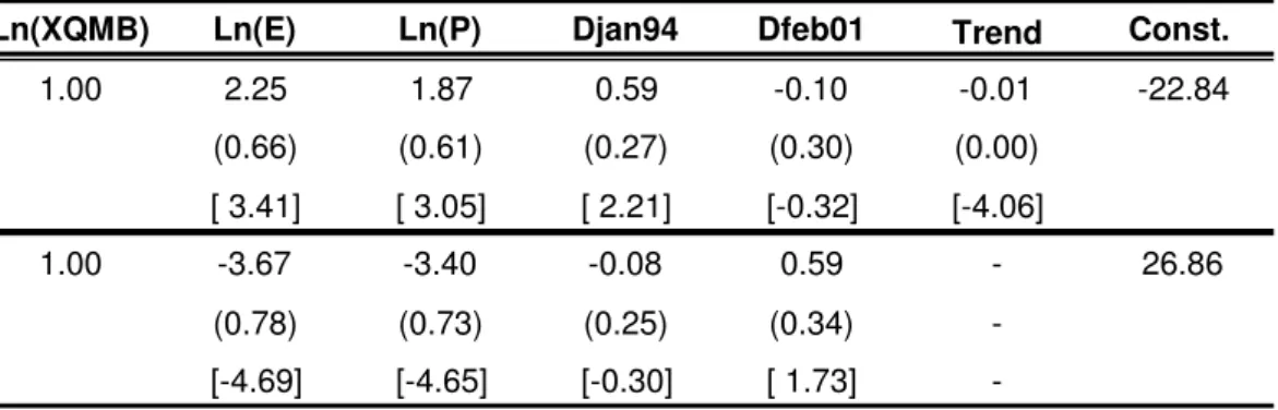
Table 7 shows the long-term estimates for the cointegration vectors under the models with trend and constant, and with only constant and two breaks: one in January 1994, and one in February 2001.
Ln(XQMB) Ln(E) Ln(P) Dsep94 Doct99 Trend Const
1.00 -0.71 -2.69 1.00 -0.65 -0.01 10.31
(0.87) (0.77) (0.35) (0.42) (0.00)
[-0.80] [3.50] [2.82] [-1.54] [1.04]
1.00 -1.81 -5.83 1.68 -1.51 - 28.85
(1.78) (1.42) (0.57) (0.80)
-Table 7: Long-term Estimates of Cointegration Vectors: Breaks in Jan/94 and Feb/01
Standard error in ( ). T statistics in [ ].
The long-term relationships in Table 7 for the model with constant and standardized for XQMB show signs opposite to those expected for the real exchange rate and international commodities prices as determinant variables of the volume of manufactured exports.
The model that disregards the trend factor in the cointegration vector presents coefficients with correct and statistically significant signs for the real exchange rate and international commodities prices. However, the dummy variables DJan94 and DFeb01, which capture information about breaks stemming from structural hysteresis theory, exhibit
coefficients that are different from expected and not statistically significant. These results suggest that the dates of the breaks (January 1994 and February 2001) have little or no influence on the long-term balance of the export sector of manufactured products.
3.2.3. Conclusions for the Brazilian Case
The results of our cointegration tests suggest a stable long-term relationship for the total volume of Brazilian exports in the absence and presence of structural breaks obtained by means of hysteresis theory. This inference suggests that the real effective exchange rate, the international commodities price, and the growth of total worldwide income captured by relevant deterministic trend terms are sufficient to determine the balance of total exports in Brazil. Thus, our test rejects the hypothesis of hysteresis to explain the behavior of total exports.
We note that the bulk of Brazilian export is of primary products—specifically, on iron mining and grains. These are commodities with no need for investment in trademarks,
reputations, local legal knowledge, and so on. Moreover, these products’ destinations are the
Ln(XQMB) Ln(E) Ln(P) Djan94 Dfeb01 Trend Const.
1.00 2.25 1.87 0.59 -0.10 -0.01 -22.84
(0.66) (0.61) (0.27) (0.30) (0.00)
[ 3.41] [ 3.05] [ 2.21] [-0.32] [-4.06]
1.00 -3.67 -3.40 -0.08 0.59 - 26.86
(0.78) (0.73) (0.25) (0.34)
-international market, since the national production of these goods considerably outstrips domestic demand. As a result, applying hysteresis theory for Brazil is quite problematic. Given its theoretical foundation, the concept of hysteresis is much more tightly connected to manufactured exports. Therefore, we conclude that this result is in line with the predictions of theory, to some extent.
The cointegration test results for manufacturing exports fail to reject the null hypothesis of absence of one or more cointegration vectors when structural breaks are disregarded. However, when breaks are inserted consistent with the theory of hysteresis, the null hypothesis of no cointegration vector has to be discarded, with preference given to the alternative of one or more cointegration vectors. Our results indicate that the long-run
equilibrium of manufactured export volume can be explained when variables that capture the effect of hysteresis are inserted, thereby corroborating the theory.
Our analysis of the estimates of the long-term cointegration vector coefficients finds, in most cases, that the signs are as expected--not only for the real exchange rate and
international commodities prices, but also for dummy variables that represent the volume of manufacturing exports. We note the role of structural breaks as identified by the theory of hysteresis in the long-term balance of the manufactured products export sector. These
estimates also reveal the best hypothesis for the dates of the breaks as suggested by hysteresis theory for September 1994, when the lower limit is redefined, and for October 1999, when the upper limit is exceeded.
4. Final Considerations
This work offers a new test for hysteresis in foreign trade. We applied this approach to the Brazilian case, in an attempt to explain the recent behavior of the international sector from the point of view of hysteresis theory.
Our proposed test combines both theoretical and empirical aspects of hysteresis models, which take into consideration sunk costs, uncertainty, and methods of analysis of cointegration with structural breaks.
and capital capture) and in planning terms (i.e., investment decisions in the long run). Such an impact can be measured by the behavior of inaction zone thresholds. Given the magnitude of the interest rate movements, thresholds respond in a significant way.
The second result of interest is the impact of elevated exchange rate uncertainty on the change of regime (from a fixed rate to a flexible rate) over the inaction zone thresholds in January 1999. The exchange rate depreciation necessary to encourage exports under a flexible exchange rate regime is more pronounced than it would be under a fixed exchange rate regime. The reason for such an effect is the drastic change in the exchange rate variance between the two periods (fixed and floating exchange rate).
It is possible to derive from these results important lessons for economic policy. First, by achieving an environment of economic stability, the competitiveness of Brazilian
companies increases in the international market. Moreover, for Brazilian competitiveness, the maintenance of macroeconomic stability based on lower volatility and on the level of real interest rates is as important as the exchange rate. An additional major economic policy prescription would be to avoid excessively volatile behavior of the exchange rate, stabilizing it as much as possible in order to reduce the costs (in the form of devaluation) of balancing the external sector.
The second stage of the test uses the results obtained in the first stage to determine when the real effective exchange rate has exceeded the inaction zone thresholds. This information was used within our cointegration methodology analysis to test the hysteresis hypothesis for the external Brazilian market.
The results of the cointegration tests with structural breaks proposed by Johansen et al. (2000) show no strong evidence of hysteresis in the case of total volume of Brazilian exports. However, tests conducted for the exports volume of manufactured products suggest evidence of hysteresis for this exporting sector. As such, we conclude that the idea of a long-term cointegration relationship may be misguided.
Our analysis of estimates of the long-term cointegration vectors’ coefficients shows the same signs as those expected from real exchange rates, for international commodities prices, and for the dummy variables, which represent structural breaks as relevant variables in the volume of manufactured exports. These relations show the role played by structural breaks in the context of hysteresis theory in respect of the long-term balance of the
Accordingly, we arrive at another important economic policy lesson. Particularly for the manufactured goods exporting sector, instead of operational or interventionist exchange rate policies, measures are necessary to improve the access of Brazilian companies to foreign markets. Such efforts could advise Brazilian companies about the peculiarities of each foreign market in terms of legislation and norms, as well as providing information about policies that ease communication with representatives and distributors. In short, we recommend policies that facilitate the logistics of the exporting process in order to reduce related costs (financial, time, etc.). Once again, we highlight the importance of economic stability for the competitiveness of Brazilian companies in foreign markets.
Although our work has investigated the subject with sufficient accuracy and proper detail, several improvements and advancements may be a focus of future research. As emphasized by Gocke (2002), "the empirical treatment of persistent economic or hysteresis effect is far from mature and requires future research. A variety of methods is applied, but none is fully accepted. So [...] the suggestion is to apply the various existing approaches and
to consider their limitations.‖ We recognize some of these limitations and we hope for
improvements in the future.
One possibility would be to work with more disaggregated sectorial data for Brazil, such as those used by Kannebley (2005); or even to work with micro-data, as Roberts and Tybout (1997) do for Colombia. A second possibility for advancing this research relates to our ability to estimate variance values over time, as in the case of averaging Brownian motion to derive the real effective exchange rate. This would improve the robustness of our inaction zone threshold estimates. The third aspect to be developed is a set of estimates for the cost parameters, especially the non-refundable costs borne by Brazilian companies related to their entry into external markets.
References
BALDWIN, R. ―Hysteresis in Import Prices: The Beachhead Effect‖. American Economic Review, 78, p. 773-785, 1988.
BALDWIN, R. ―Sunk-cost Hysteresis‖. NBER Working Paper 2911, março de 1989.
BALDWIN, R. e KRUGMAN, P. ―Persistent Trade Effects of Large Exchange Rate Shocks‖.
CONFEDERAÇÃO NACIONAL DA INDÚSTRIA. ―Valorização do Real Provoca Mudança na Estrutura de Comércio Exterior da Indústria‖. Sondagem Especial, ano 4, n. 2, junho de 2006.
DIXIT, A. ―Hysteresis, Import Penetration, and Exchange Rate Pass-Through‖. The Quarterly Journal of Economics, vol. 104, n. 2, p. 205-228, maio de 1989a.
________. ―Entry and Exit Decisions under Uncertainty‖. Journal of Political Economy, vol.
97, n. 3, p. 620-38, junho de 1989b.
________. ―Hysteresis and the Duration of the J-curve‖. Japan and the World Economy, 6, p.105-115, 1994.
DOORNIK, J. A. ―Approximations to the Asymptotic Distributions of Co integration Tests‖.
Journal of Economic Surveys, 12, p. 573-593, 1998.
ENDERS, W. ―Applied Econometrics Time Series‖. John Wiley & Sons, 2nd edition, 2004.
GOCKE, M. ―Various Concepts of Hysteresis Applied in Economics‖. Journal of Economic
Surveys, vol.16, n.2, p.167-88, 2002.
HALLETT, A. J. H. e PISCITELLI, L. ―Testing for Hysteresis Against Nonlinear Alternatives‖. Journal of Economic Dynamics & Control, 27, p. 303-327, 2002.
HARVEY. A. C. ―Forecasting, Structural Time Series and the Kalman Filter‖. Cambridge
University Press, 1989.
JOHANSEN, S. ―Statistical Analysis of Co integration Vectors‖. Journal of Economic
Dynamics and Control, 12, p. 231–254, 1988.
________. ―Likelihood-based Inference in Co integrated Vector Autoregressive Models‖. Second printing, Oxford University Press, 1996.
JOHANSEN, S., MOSCONI, R. e NIELSEN, B. ―Co integration Analysis in the Presence of
Structural Breaks in the Deterministic Trend‖. Econometrics Journal, vol 3, p.216-249, 2000.
KANNEBLEY, S. Jr. ―Testes para Hipótese de Hysteresis em Exportações Industriais
Brasileiras: Uma Análise de Cointegração Limiar. Working Paper apresentado no seminário de economia da EESP-FGV em 28/09/2005.
KRUGMAN, P. e BALDWIN, R. ―The Persistence of the US Trade Deficit‖. Brookings
Papers on Economic Activity, 1, 1987.
LÜTKEPOHL, H. e KRÄTZIG, M. ―Applied Time Series Econometrics‖. Cambridge
University Press, 2004.
Cambridge University Press, 1998.
PERRON, P. ―Dealing With Structural Breaks‖. Paper preparado para Palgrave Handbook of
Econometrics, vol 1, Econometric Theory. Versão de 20 de abril de 2005.
ROBERTS, M. J. e TYBOUT, J. R. ―The Decision to Export in Colombia: An Empirical Model of Entry with Sunk Costs‖ The American Economic Review, vol. 87, n. 4, p. 545- 564, setembro de 1997.
TELES, V. K. ―Choques Cambiais, Política Monetária e Equilíbrio Externo da Economia
Brasileira em um Ambiente de Hysteresis‖. Economia Aplicada, vol. 9, n. 3, p. 415-426, jul-set 2005.
WELCH, G. e BISHOP, G. ―An Introduction to the Kalman Filter‖. University of North