© 2014 The El-Adawy, A., A.M. Negm, O.C. Saavedra V, K. Nadaoka and I.A. El-Shinnawy. This open access article is
Original Research Paper
Coupled Hydrodynamic-Water Quality Model for Pollution
Control Scenarios in El-Burullus Lake (Nile Delta, Egypt)
1El-Adawy, A., 1A.M. Negm, 1,2O.C. Saavedra V, 1,3K. Nadaoka and 4I.A. El-Shinnawy
1
Department of Environmental Engineering, Egypt-Japan University of Science and Technology E-JUST, New Borg El-Arab, Alexandria, Egypt
2Department of Civil Engineering, Graduate School of Science and Engineering, Tokyo Institute of Technology, Tokyo 3
Department of Mechanical and Environmental Informatics, Graduate School of Information Science and Engineering, Tokyo Institute of Technology, Tokyo, Japan
4
Coastal Research Institute, Alexandria, Egypt Article history Received: 2014-01-03 Revised: 2014-02-09 Accepted: 2014-10-25 Corresponding Author: A.El-Adawy,
Department of Environmental Engineering, Egypt-Japan University of Science and Technology E-JUST, New Borg El-Arab, Alexandria, Egypt
E-mail:
Abstract: El-Burullus Lake is affected by increasing and extensive human
activities, rapid social-economic development and the construction of fish ponds nearby. This has significantly impacted the health of the lake eco-system. On the foundation of the two-dimensional depth averaged hydrodynamic model, distributions of the salinity, Dissolved Oxygen (DO), Biochemical Oxygen Demand (BOD), Chemical Oxygen Demand (COD) and Ammonium (NH4) were
modeled. The heat flux model was also utilized to enhance the accuracy of the calculations in the water quality modeling stage. The calibration and the verification of this model were based on spatially distributed water quality measurements during the period 2010-2011. The correlation coefficients between measured and simulated salinity was found to be 0.79 in January 2011 and 0.84 in August 2010 with a mean errors of 1.3407 and 2.0727 ppt in August 2010 and January 2011 respectively. The results generally agree with the observations, but this indicates that more measurements are needed to verify the predictability of the simulations. In addition, Delft-3D model has been applied in evaluating the feasibility of adding a new artificial inlet or diversion of some drains. The model proved to be an effective tool for the water dynamics, water quality simulation and evaluating different scenarios of such shallow Lake.
Keywords: Hydrodynamics, Coupling, Water Quality Modeling, Shallow Lakes,
El-Burullus, Scenario Analysis
Introduction
Terrestrial lakes contain 90% of liquid freshwater on the Earth’s surface and are critical elements of the water cycle, as they sustain aquatic biodiversity and provide the livelihoods as well as the social, economic and aesthetic benefits essential to quality of life in lake catchment communities (Xu et al., 2012). The aim of modeling surface water quality is to construct a mathematical model of a stream (flowing water), making it possible to track changes in water quality according to the initial and boundary conditions of the simulation. Modeling of water quality problems allows analysis of phenomena and the dependencies between them in order to predict and quantify the effects of changes in the aquatic environment (Ziemińska-Stolarska and Skrzypski, 2012). Since the 1970 s, some large shallow
Zhao et al. (2013) utilized the Environmental Fluid Dynamics Code (EFDC) to represent the main water quality and ecological processes in Lake Yilong (China). The calibrated and validated model was used in different scenarios to understand the water quality responses to various load reductions and ecological restoration measures. With developments in computing techniques (Ashraf et al., 2012), more water quality models have been developed with various model algorithms. Mittelstet et al. (2012) built a simplified Graphic User Interface for Soil and Water Assessment Tool to identify areas that likely contributed disproportionate amounts of Phosphorus (P) and sediment to Lake Overholser (USA). To date, tens of types of water quality models including hundreds of models have been developed for different topographies, water bodies and pollutants at different spatial and temporal scales. However, the results often show considerable variance due to the differing theories and algorithms used in the models. The modeling results cannot be reliably compared to each other and the inconsistent findings support differing environmental management options (Obropta et al., 2008). The goal of the present study is to make a start in modeling the hydrodynamics and the water quality in El-Burullus Lake. The study is organized as follows: Study area is discussed in section 2. Modeling framework is described in section 3. In Section 4, Discussion and conclusions are presented.
Study Area
El-Burullus Lake is a coastal lagoon located in the central Nile Delta (Longitude 30° 30° and 31°10° E and latitude 31° 21° and 31° 35° N). The lagoon is 65 km long by approximately 5 km wide, covering a water surface area of 410 km2. The water is shallow and brackish, with a depth of 0.42 to 2.07 m (Younes and
Nafea, 2012). As seen in Fig. 1, the lake is connected to the Mediterranean Sea by Al Boughaz, a small outlet about 80 m wide near the village of El Burg. Figure 1 also describes the land uses around and within the lake.
Since 1965, pollution and eutrophication have increasingly threatened the ecosystem of the region (Chen et al., 2010). There are nine inflowsinto El-Burullus Lake, discharging approximately 3904 million m3/year, including agricultural, industrial and domestic waste water (Abayazid and Al-Shinnawy, 2012). The lake receives runoff from agricultural areas and inputs via eight drains in addition to fresh water from Brimbal Canal situated in the western part of the lake. The main water quality problems are declining salinity level and associated deterioration in aquatic ecosystem and declining marine fish population (Abayazid and Al-Shinnawy, 2012). Aquatic pollutants include industrial chemicals that are indicative of industrial growth in the region. The lake’s nutrient-rich environment promotes growth of aquatic plants. The subsequent sediment accumulation around plant roots effectively sub-divides the lake and affects the water circulation. In addition, Total Suspended Solids (TSS) values are very high, indicating high pollution by organic and non-organic matter from industrial and agriculture waste. The declining salinity of the lake is considered a problem: Total percentage by weight of marine fish species such as Liza ramada decreased from 16% in 1973 to less than 1.8% in 2003 and freshwater species such as Tilapia increased from about 81 to 98.2% (Al Sayes et al., 2007). Figure 2A shows one of the drains discharging into the lake, while Fig. 2B indicates the shallowness of the lake. Despite its self-purification capacity and increase in the number of aquatic plants, the environmental quality of water in El-Burullus Lake had been deteriorating.
Fig. 2. (A) Drain No.9 at Shakhloba village on the Lake coast. (B) The shallowness of the lake
The first stage of the research included creating a validated hydrodynamic model using available data sets. The model was used to examine a potential mitigation scenario by decreasing the pollutant loads entering the lake, i.e., diversion of existing inflows (El-Adawy et al., 2013). This study forms the second stage of an integrated management strategy for El-Burullus Lake, which assesses the current situation and employs scenario analysis of potential pollution control measures. In this study, the study areaand modeling configurations are described; then, the method is described and parameter estimation is considered. The final stage examines the validity of the calibrated water quality models and forecasts the behavior of the lake under different management scenarios.
Modeling Framework
Delft3D-WAQ Model
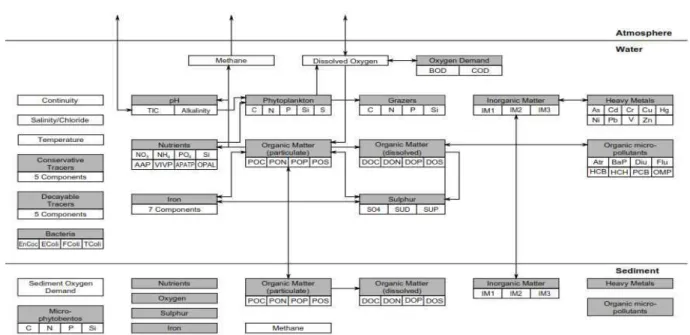
Delft3D-WAQ is a three-dimensional water quality model framework. It solves the advection-diffusion-reaction equation on a predefined computational grid for a wide range of modeled substances. Delft3D-WAQ allows great flexibility in the substances to be modeled, as well as in the processes to be considered, as shown in Fig. 3. Hydrodynamic modeling usually requires a more detailed schematization or grid than water quality modeling. Therefore, it is generally allowed to reduce the number of computational cells in water quality modeling via aggregation in both the horizontal and vertical directions. The results calculated in the Delft3D-FLOW module (such as velocities, water elevations, density, salinity, vertical eddy viscosity and vertical eddy diffusivity) are used as inputs for Delft3D-WAQ via a coupling process.
Delft3D-WAQ solves the equations for transport and physical, (bio) chemical and biological processes. Delft3D-WAQ reproduces the mass balance of the selected state variables for each computational cell. The mass transported by water from one cell to another is a negative term for the first computational cell and positive for the second (receiving) computational cell.
Delft3D-WAQ solves Equation 1 for each computational cell and state variable, which is a simplified representation of the advection-diffusion-reaction equation:
t t t
i i
Tr p s
M M M
M M t t t
t t t
+∆ = + ∆ ∆ + ∆∆ + ∆ ∆
∆ ∆ ∆
(1)
Where:
• Mass at the beginning of a time step t t i
M +∆
• Mass at the end of a time step • Changes by transport:
Tr M t t ∆ ∆ ∆
• Changes by physical, (bio) chemical or biological
processes: P M t t ∆ ∆ ∆
• Changes by sources
S M t t ∆ ∆ ∆
Configuration of Delft3D-WAQ Model
Grid Generation
A curvilinear grid was developed to discretize El-Burullus Lake. A grid of finite difference quadrangular elements was created for the entire lake with about 66000 cells, as shown in Fig. 4A, which also shows the positions of the drains. The grid resolution ranges from 20 to 270 m (El-Adawy et al., 2013). The water quality modeling stage starts with the coupling process, in
which the Delft3D-WAQ module utilizes the
hydrodynamic conditions and parameters (velocities, water elevations, density, salinity, vertical eddy viscosity and vertical eddy diffusivity) calculated in the Delft3D-FLOW module.
3.3. Defining Substances and Parameters
Fig. 3. Substances included in Delft3D-WAQ. (After Delft3D-WAQ manual, 2011)
(A)
(B)
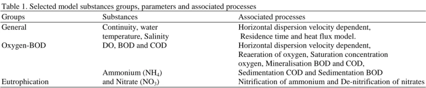
Table 1. Selected model substances groups, parameters and associated processes
Groups Substances Associated processes
General Continuity, water Horizontal dispersion velocity dependent,
temperature, Salinity Residence time and heat flux model.
Oxygen-BOD DO, BOD and COD Horizontal dispersion velocity dependent,
Reaeration of oxygen, Saturation concentration oxygen, Mineralisation BOD and COD,
Ammonium (NH4) Sedimentation COD and Sedimentation BOD
Eutrophication and Nitrate (NO3) Nitrification of ammonium and De-nitrification of nitrates
Data Collection and Processing for the Coupled
Model
All the data required by the coupled model were collected and then processed. The calibration and validation of the hydrodynamic model utilized components of the hydrodynamic data sets (drain discharge, water leveland tidal variation) and meteorological data sets (wind vectors, solar radiation, relative humidity and temperature). In addition, geometric data (bathymetry, land boundaries, island boundaries and inlets positions) were used in determining the closed and open boundaries of the model and in creating the grids (El-Adawy et al., 2013).
In the previous stage of the research (El-Adawy et al., 2013), these data helped in building and validating the hydrodynamic model of El-Burullus Lakeand provides the basis for the water quality modeling stage. The present study represents the second stage of the research. The Drainage Research Institute monitors the quantity and quality of agricultural drainage water in the Nile Delta and Fayoum region. DRI data were obtained on the pollutant loads entering the lake from drains during a one-year period from mid-June 2010 to mid-July 2011. The quality parameters comprise organic contamination, chemical composition, salinity and other physical properties (Shaban et al., 2010). The physical and chemical characteristics of the waters near the sea inlet, that are required to establish the open boundary of the model, are taken from periodical reports published by the Egyptian Environmental Affairs Agency (EEAA, 2011).
Circulation patterns provide the basis for the water quality modeling stage. Figure 4B shows the spatial distribution of velocity magnitude and direction on 31 October 2010 and shows that the maximum velocity occurs at the inlet and drain outfall locations.
Modeling Procedure
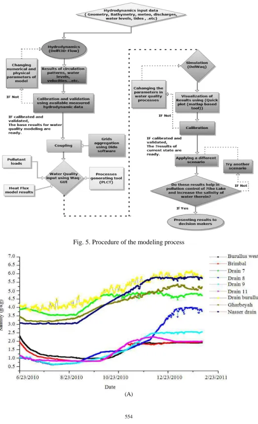
Figure 5 shows the modeling procedure used for the whole study. Firstly, as discussed previously, the hydrodynamic model is calibrated and validated using the available data sets then a coupling process is applied to make the hydrodynamic results suitable for the water quality modeling stage. The main steps in developing the water quality model involve: Aggregation of grids; defining initial conditions, boundary conditions, waste
loads, simulation time, output variables; and determining the monitoring stations. The PLCT was used to define the substances and water quality processes to be included in the mode. The model is calibrated and validated to ensure that it adequately represents the present state of the lake. The validated model is used to predict water quality parameters under different future scenarios. Based on the predicted outcomes, engineering solutions which ensure appropriate hydrodynamic and water quality criteria could be presented to decision makers.
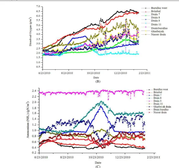
Figure 6A-C show examples of the pollutant loads and water characteristics immediately prior to entering the lake: The salinity at each drain inlet just before entering the lake (Fig. 6A); DO at nine locations during the same period (Fig. 6B); Ammonium (NH4)
concentrations entering the lake (Fig. 6C).
Model Boundary Conditions and Monitoring
Stations
After many trials, the initial conditions were selected to be 1 for continuity, 4 g Kg−1 for salinity, 5 g/m3 for Dissolved Oxygen, 0.5 for Ammonium NH4,
0.05 gN/m3 for Nitrate NO3, 25 gO2/m3 for BOD and
15 gO2/m3 for COD. The heat flux model results in the
previous study were used to define the spatial and temporal distribution of temperature in the same period of simulation. The model time frame was selected as the same period for the hydrodynamic modeling, started from 23 June 2010 until 15 March 2011. The time step selected for the water quality model was set to 30 min. The boundary conditions assigned for the open boundary included all values of water quality parameters measured in the same period. To calibrate the model, monitoring stations were established at the same locations (Fig. 7) for the field samples and the evaluation processes, in order to compare the measured water parameters with the model predictions.
Model Calibration
and NH4. The data set used for calibration is from a
comprehensive field sampling campaign conducted in El-Burullus Lake during the same period as the data set provided by DRI (Younes and Nafea, 2012).
Applying Scenarios to Control Lake Pollution
The final step in the study is to test various scenarios in order to assess different engineering solutions to control
pollution in El-Burullus Lagoon. One scenario involves constructing another artificial inlet with an average depth of 2 m to increase exchange rates between the lake and the Mediterranean Sea. Another approach would be to divert some drains from discharging into the lake to the west branch of the Nile in order to control lake pollution and at the same time address the problem of sediment accumulation at the Rosetta mouth of the Nile.
Fig. 5. Procedure of the modeling process
(B)
(C)
Fig. 6. (A) Time series data of salinity at drains (B) Time series data of Dissolved oxygen at drains (C) Time series data of Ammonium (NH4) at drains
Results
Calibration Results
Checking Numerical Accuracy and Stability of the
Simulation
Continuity is a special conservative tracer. It is used to check the accuracy and stability of the simulation. Every drain in the model is set to have a continuous concentration of 1 g/m3 and the open boundaries also have a similar continuity constant. Any deviation from the value of 1 g/m3 at any monitoring station indicates numerical error during simulation. Figure 8 shows the mass balance results at different locations in the lake. Figure 8A shows the results in case of excluding the effect of evaporation before coupling the hydrodynamic results. If evaporation is included, continuity shows higher concentration due to the loss of pure water during evaporation. Figure 8B shows the results of including evaporation in the hydrodynamic model.
Model Calibration Results
Calibration of Salinity Parameters (General
Group)
As a conservative substance, salinity as is only subject to transport but, unlike decayable substances, is not subject to water quality processes. Salinity level can isolate the effect of transport and thereby help to distinguish between the effect of transport and processes for other substances.While simulating salinity, a velocity-dependent horizontal dispersion process is added as an active process. One of the most important parameters in this process is ‘background dispersion’. The range used to calibrate salinity is from 0.1 to 10 m2/s. The simulated values are compared with the spatial distribution of salinity observed in August and January. Table 2 shows the results of the calibration analysis for parameters in
salinity substances.
(A)
(B)
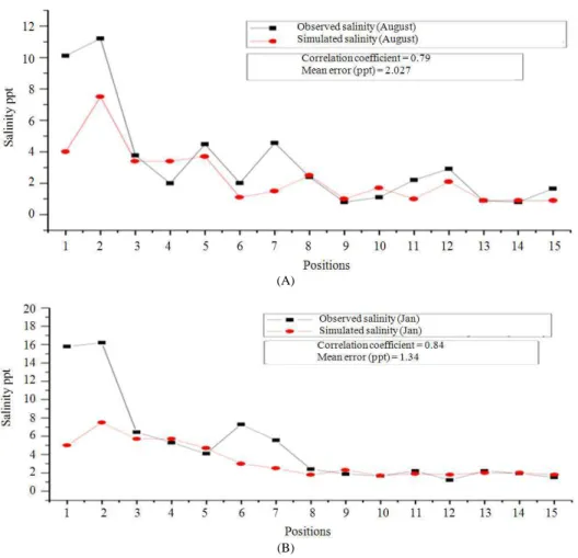
Figure 9 shows the simulated salinities at station 2 using different values for background dispersion. The results of the calibrated model are presented in Fig. 10A and B in whichbackground dispersion (Dback) was
set to 0.1 m2/s. The mean error is 1.3 ppt in August and 2.0727 ppt in January. The deviation occurs mainly at locations near Boughaz, due to the dynamic
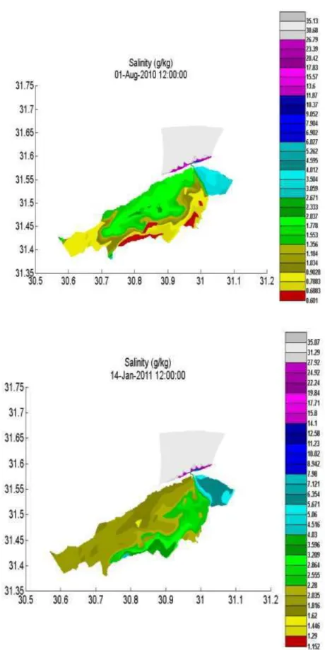
effect of tide on the behavior of water approaching the inlet. Figure 11 shows the spatial distributions of simulated salinity in August and January. The simulated results show good agreement with the field measurements (correlation coefficients 0.79 and 0.84), where the ranges of salinity are between 10.6 and 1.37 g kg−1.
Fig. 9. Simulated salinities at station 2 using different values of background dispersion
(A)
(B)
Calibration of Water Quality Parameters
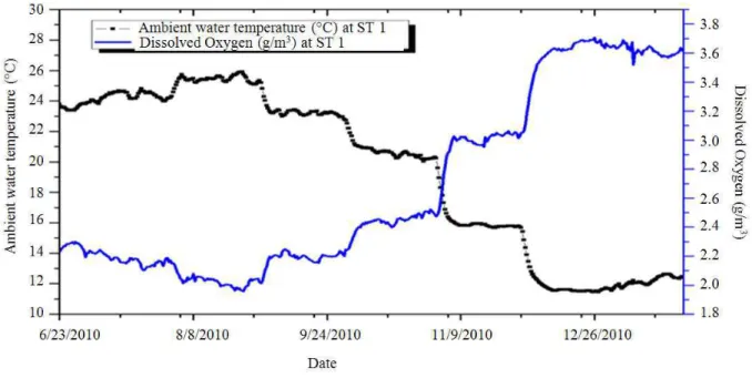
Adequate concentrations of dissolved oxygen are critical to the health of lacustrine biota. The oxygen saturation level depends on water temperature, among other variables (Smith et al., 2001). Therefore, the results of the heat flux model, which include the spatiotemporal distribution of water temperature, were
introduced as inputs to the model. Once absorbed, oxygen is either incorporated throughout the water body via internal currents or is lost from the system. Flowing water is more likely to have high DO levels than is stagnant water because of the water movement at the air-water interface (Radwan et al., 2003). Figure 12 shows DO concentration in relation to ambient water temperature.
Fig. 12. DO and ambient water temperature relationship at station 1
(B)
(C)
Fig. 13. (A) Simulated and Observed DO in August 2010. (B) Simulated DO during the simulation time at 7 stations inside the Lake. (C) Spatial distribution of DO on 10th of January 2011
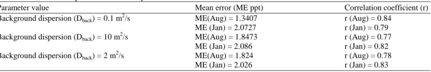
Table 2. Calibration for parameters in salinity substance
Parameter value Mean error (ME ppt) Correlation coefficient (r)
Background dispersion (Dback) = 0.1 m2/s ME(Aug) = 1.3407 r (Aug) = 0.84
ME (Jan) = 2.0727 r (Jan) = 0.79
Background dispersion (Dback) = 10 m2/s ME(Aug) = 1.8473 r (Aug) = 0.77
ME (Jan) = 2.086 r (Jan) = 0.82
Background dispersion (Dback) = 2 m2/s ME(Aug) = 1.824 r (Aug) = 0.78
Not only dissolved oxygen but all other water quality parameters depend mainly on water temperature. Many parameters were tuned in each substance. The most important parameters are shown in Table 3, which presents statistical analysesfor the model simulations that most closely matched the observed data. The simulation results were assessed via Mean Error (ME) and correlation coefficient (r). The most important coefficients shown in Table 3 are reaeration transfer coefficient, temperature coefficient for reaeration, decay rates of Biological Oxygen Demand (BOD), nitrification rate at 20°C and temperature coefficient for nitrification. An accepted mean error for DO is about 0.875 mg L−1. Figure 13A shows the measured and simulated DO at different location in the lake. Figuer 13B shows simulated DO at seven stations. Figure 13C shows the spatial distribution of DO on 10 January 2011.
Biological Oxygen Demand (BOD) represents the amount of oxygen consumed by microorganisms in order to break down organic matter and reflects the potential consumption of DO. BOD5, which is
simulated in this study, refers to BOD measured at a temperature of 20°C after 5 days incubation (in
darkness, to prevent production of DO via
photosynthesis. The calibrated results shown in Fig. 14A indicate that the model underestimated BOD at some stations, especially in the central area of the lake, but the predictions still follow the general trend in the observed data, with a mean error of 7.54 mg L−1 and correlation coefficient of 0.6113. As seen in Fig. 14B, simulated BOD at eight stations distributed across the lake was between 4 and 39 gO2/m
3
. The decay rate for the calibrated BOD model was set to 0.08 d−1.
(A)
(B)
(A)
(B)
Fig. 15. (A) Simulated results of COD at 8 stations. (B) Spatial distribution of COD on 11th of October 2010
Table 3. Calibration For important parameters in main water quality processes
Run ID Parameters values Mean Error (ME) Correlation coefficient (r)
DO_1 *Reaeration transfer coefficient (KLrear m/d) = 0.5 0.875 mg L−
1
0.615 Temperature Coefficient for Reaeration (TCrear) = 1.016
DO_2 Reaeration transfer coefficient (KLrear m/d) = 1.0 1.92 mg L−1 0.200
Temperature Coefficient for Reaeration (TCrear) = 2.0
DO_3 Reaeration transfer coefficient (KLrear m/d) = 1 1.04 mg L−1 0.475
Temperature Coefficient for Reaeration (TCrear) = 1.016
BOD_1 *Decay rate BOD = 0.08 7.54 gO2/m
3
0.611
BOD_2 Decay rate BOD = 0.15 11.8 gO2/m3 0.554
BOD_3 Decay rate BOD = 0.3 17.12 gO2/m3 0.490
NH4_1 *Nitrification rate at 20°C RcNit; gN/m3/d = 0.1 0.224 gN/m3 0.683
Temperature Coefficient for nitrification TCNit 20 = 1.07
NH4_2 Nitrification rate at 20°C RcNit; gN/m3/d = 0.5 0.18 gN/m3 0.442
Temperature Coefficient for nitrification TCNit 20 = 1.2
NH4_3 Nitrification rate at 20°C RcNit; gN/m3/d = 0.5 0.32 gN/m3 0.380
(A)
(B)
(C)
Fig. 16. (A) A comparison between measured and simulated values of ammonium (NH4). (B) The spatial distribution of NH4on 22th
Chemical Oxygen Demand (COD) is the amount of oxygen required to oxidize all pollutants. Simulated COD at eight stations is shown in Fig. 15A. The decay rate (RcCOD) factor, which is the most effective in the
mineralization process, is set to 0.05 d−1. The spatial distribution of COD on 11 October 2010 is shown in Fig. 15B. Similar to BOD, the concentrations are highest near drain outfalls and decrease with increasing distance from these locations.
Generally, ammonium is one of the most active and important components of the N cycle in aquatic ecosystems. Despite low ambient concentrations in many water bodies, ammonium can still be a major source of N for autotrophs and microbes (Kumar et
al., 2007). Figure 16A compares measured and
simulated values of ammonium (NH4), showing the
highest concentrations in the area around drains 8 and 9. The nitrification rate at 20°C (RcNit) is set to 0.1
gN/m3/d where the temperature coefficient for nitrification (TCNit) was 1.07. The mean error of the
simulated results was 0.224 gN/m3 where the correlation coefficient was 0.683. The spatial distribution of ammonium is shown in Fig. 16B. As seen in Fig. 16 C, of eight stations the highest simulated ammonium concentration occurs at station 9 and the lowest at station 7.
Analysis of Model Response to Suggested
Engineering Scenarios
Adding a new Inlet (Boughaz)
The simulation results predict that the construction of a new inlet would help increase salinity in the lake (Fig. 17A).
Load Reduction Scenario
The findings indicate that it is unfavorable to divert all drains from the same area. Therefore, it is suggested to divert drains 7, 8 and 11 so that no adjacent drains are diverted. Figure 17B shows the effect of diverting the drains on the spatial distribution of salinity.
In the case of diverting the drains, the simulation shows that DO will reach 6.5 g/m3 with an average increase of approximately 1 g/m3. Figure 18A shows the increase in DO at a monitoring station in the west part of the lake. Figure 18B shows the decrease in BOD due to the reduction in pollutant loads entering the lake. Figure 18C shows the effect of diverting three of the eight drains on the spatial distribution of ammonium.
Discussion
Checking numerical accuracy and stability of the simulation results indicate that, before conducting the mass balance test, it is necessary to consider whether to take evaporation into consideration in order to avoid misleading results. In Delft3D-WAQ module, the constituents of a water system are divided into functional groups. A functional group includes one or more substances that display similar physical and/or (bio) chemical behavior in a water system. In the present study, all constituents are categorized under three main groups. These groups are general group, oxygen group and eutrophication group. The parameters in the main three groups were modeled. DO, BOD and COD parameters were modeled in the oxygen group.
(B)
(A)
(B)
(C)
From the spatiotemporal distributions of simulated DO, it is noticeable that the lowest values (generally less than 2 mg L−1) are near the drain outfalls. Reaeration and self-purification processes occur in the lagoon, resulting in DO concentrations of up to 6 mg L−1 at locations remote from the drain inlets.
The increase in salinity levels in the lake after adding a new inlet occurs due to increased exchange rates between the lake and the Mediterranean Sea. The increase in salinity is only noticeable in the area around El-Boughaz.
The diversion of any drain discharging into the lake will lead directly to a decrease in water level. Quantitative and qualitative analysis of potential management strategies can help identify the optimum diversion scenario that maintains water levels within acceptable ranges while also controlling pollution.
Conclusion
Hydrodynamic results were successfully used as inputs to a coupled water quality model. Two updated data sets (2010-2011) from different sources were used, permitting the simulation period to be extended to the years 2010-2011. Following appropriate calibration, the models provide reasonable results.
The findings show that:
• Prior to the coupling process, the numerical errors in the hydrodynamic model averaged 0.02%
• The flow patterns in the lake are the main factors affecting the spatiotemporal distribution of pollutants • The water quality state variables, salinity, DO,
COD, BOD and NH4 modeled in the study are
dependent upon the concentration of effluent inputs from various inlets
• The measured and simulated salinity had a correlation coefficient of 0.84 in August 2010 and 0.79 in January 2011, mean errors of 1.3407 ppt and 2.0727 ppt in August 2010 and January 2011 respectively • The shallowness of El-Burullus Lake and the
retention time of 28 to 45 days enhanced the self-purification capacity of the lake
• Developing a heat flux model enhances the accuracy of the results, because all water quality parameters, especially dissolved oxygen, are highly sensitive to water temperature
• The gradients of pollutant concentrations indicate that the areas near drain outfalls are the most polluted areas of the lake
Some factors should be considered in future modeling of Lake Burullus, such as including suspended sediment concentrations, Chlorophyll-a (CHL-a) and phosphorous compounds. Permanent monitoring stations distributed throughout the lake are required for continuous and well distributed records of the hydrodynamic, physical and chemical properties of the lake waters.
Acknowledgment
The first researchers is supported by a scholarship from the Mission Depa f the Government of Egypt which is gratefully acknowledged. He is also grateful for his earlier supervisor Dr. Mohammed El-Zier who passed away on August 2012. Last, but not least I am thankful to Egypt-Japan University of Science and
Technology (E-JUST) and Japan International
Cooperation Agency (JICA) for offering the tools and equipment needed for the research work.rtment, Ministry of Higher Education.
Additional Information
This study was partially funded by JSPSCore-to-Core Program, B.Asia-Africa Science Platforms.
This research was undertaken when Eng. Ahmed El-Adawy was a master student at Environmental Engineering Dapartment at Egypt-Japan University of Science and Technology (E-JUST). Prof. Abdelazim Negm was the main supervisor of his master thesis. Dr. Oliver saavedra and Prof.Ibrahim ElShinnawy were co-supervisors of his thesis. Prof. Nadaoka supported this study by improving the methodology used in this study.
References
Abayazid, H. and I. Al-Shinnawy, 2012. Coastal lake sustainability: Threats and opportunities with climate change. IOSR J. Mechanical Civil, 1: 33-41. Al Sayes, A., A. Radwan and L. Shakweer, 2007. Impact of drainage water inflow on the environmental conditions and fishery resources of lake borollus. Egypt. J. Aquat. Res., 33: 312-321.
Ashraf, M.A., M. Maah and I. Yusoff, 2012. Morphology, geology and water quality assessment of former tin mining catchment. Sci. World J. PMID:22761549
Azab, A.M., 2012. Integrated GIS, remote sensing and mathematical modeling for surface water quality management in irrigated water sheds. Ph.D. Delft University of Technology, Delft, the Netherlands. Bertram, P.E., 1993. Total phosphorus and dissolved
oxygen trends in the central basin of lake erie, 1970-1991. J. Great Lakes Res., 19: 224-236. DOI: 10.1016/S0380-1330(93)71213-7
Chen, Z., A. Salem, Z. Xu and W. Zhang, 2010.
Ecological implications of heavy metal
concentrations in the sediments of Burullus Lagoon of Nile Delta, Egypt. Estuar. Coast. Shelf Sci., 86: 491-498. DOI:10.1016/j.ecss.2009.09.018
EEAA, 2011. Second sampling campaign for
El-Adawy, A., A.M. Negm, M.A. Elzeir, O.C. Saavedra and I.A. El-Shinnawy et al., 2013. Modeling the hydrodynamics and salinity of el-burullus lake (nile delta, Northern Egypt). J. Clean Energy Technol., 2: 157-163. DOI:10.7763/JOCET.2013.V1.37
Kumar, S., R.W. Sterner, J.C. Finlay and S. Brovold, 2007. Spatial and temporal variation of ammonium in lake superior. J. Great Lakes Res., 33: 581-591. DOI:10.3394/0380-1330(2007)33
Mittelstet, A., E. Daly, D. Storm, M. White and G. Kloxin, 2012. Field scale modeling to estimate phosphorus and sediment load reductions using a newly developed graphical user interface for soil and water assessment tool. Am. J. Environ. Sci., 8: 605-614. DOI: 10.3844/ajessp.2012.605.614 Obropta, C.C., M. Niazi and J.S. Kardos, 2008.
Application of an environmental decision support system to a water quality trading program affected by surface water diversions. Environ. Manage., 42: 946-956. DOI:10.1007/s00267-008-9153-z
Radwan, M., P. Willems, A. El-Sadek and J. Berlamont, 2003. Modelling of dissolved oxygen and biochemical oxygen demand in river water using a detailed and a simplified model. Int. J. River Basin
Manage., 1: 97-103. DOI:
10.1080/15715124.2003.9635196
Shaban, M., B. Urban, E. Saadi and M. Faisal, 2010. Detection and mapping of water pollution variation in the Nile Delta using multivariate clustering and GIS techniques. J. Environ. Manage., 91: 1785-93. DOI:10.1016/j.jenvman.2010.03.020
Smith, R.L., T.M. Smith, R.A. Desharnais, J. Bell and M.A. Palladino et al., 2001. Ecology and field biology. Benjamin Cummings San Francisco. Xu, L., J. Pan, J. Jiang, H. Zhao and C. Liu, 2012. A
history evaluation modelling and forecastation of water quality in shallow lake. Water Environ. J., 27: 514-523.DOI: 10.1111/j.1747-6593.2012.00370.x Younes, A.M. and E.M. Nafea, 2012. Impact of
environmental conditions on the biodiversity of mediterranean sea lagoon, Burullus Protected Area, Egypt. World Applied Sci. J., 19: 1423-1430. Zhao, L., Y. Li, R. Zou, B. He and X. Zhu et al., 2013. A
three-dimensional water quality modeling approach for exploring the eutrophication responses to load reduction scenarios in Lake Yilong (China).
Environ. Pollut., 177C: 13-21. DOI:
10.1016/j.envpol.2013.01.047