!
" #
$
%&
' (
% )
* %
+
,
In‡ation and Income Inequality: A
Shopping-Time Approach (Forthcoming, Journal
of Development Economics)
Rubens P. Cysne, Wilfredo Maldonado and Paulo Klinger Monteiroy.
September 10, 2004
Abstract
Our work is based on a simpli…ed heterogenous-agent shopping-time economy in which economic agents present distinct productivities in the production of the consumption good, and di¤erentiated access to transacting assets. The purpose of the model is to investigate whether, by focusing the analysis solely on endogenously determined shopping times, one can generate a positive correlation between in‡ation and income inequality. Our main result is to show that, provided the pro-ductivity of the interest-bearing asset in the transacting technology is high enough, it is true true that a positive link between in‡ation and income inequality is generated. Our next step is to show, through analysis of the steady-state equations, that our approach can be inter-preted as a mirror image of the usual in‡ation-tax argument for income concentration. An example is o¤ered to illustrate the mechanism.
The authors are thankful for comments of participants in workshops at the University of Chicago and at the Graduate School of Economics of the Getulio Vargas Foundation (EPGE/FGV). The authors also thank the editor for his remarks, which improved the …nal version of the paper. Keywords: In‡ation, Gini Coe¢cient, Income Inequality, Shopping Time, Income Distribution. JEL: E40, D60
yRubens Penha Cysne is a Professor of Economics at the Graduate School of Economics
1
Introduction
Although there remains some controversy in the empirical literature relating in‡ation to income distribution (which Galli and Hoeven (2001) call "the in‡ation-income inequality puzzle"), several works (e.g., Bulir (2001), Romer and Romer (1998), Easterly and Fischer (2001)) present evidence correlating high rates of in‡ation with income inequality and/or poverty.
This literature, however, still lacks optimizing dynamic models capable of delivering such a result from theoretical standpoints.
The connection between in‡ation and income inequality is usually made, on descriptive grounds, by claiming that the poor1, having more restricted access to interest-bearing moneys, end up paying a higher proportion of their income as in‡ation tax2. Here we do not pursue such a channel directly. We maintain the hypothesis that the poor have more restricted access to …nancial assets. But instead of focusing on the di¤erentiated (negative) real interest rates paid by transacting balances, we concentrate on the di¤erent shares of time allocated as shopping time, by rich and by poor, due to the existence of in‡ation. Since this shopping time is actually a measure of the welfare costs of in‡ation (Lucas (2000), Cysne (2003)), our approach can be interpreted as investigating whether the welfare costs of in‡ation, by a¤ecting the poor more than the rich, can concentrate income.
It turns out that, in equilibrium, the shopping time spent by consumers in order to save on the use of transacting balances, is a mirror image of the amount of real interest payments on these same balances, on account of in‡ation, in the process of maximizing discounted utility. Intuitively, this fact, noted by Lucas (1993, p. 14, eq. 4.14)3, can be explained in terms of an equalization between marginal costs and marginal bene…ts. Formally, it is presented later, in a generalization of Lucas’s argument, by equations (15) and (16). We shall come back to this point in Section 5 of this paper.
The fact that shopping times are, under the formalization described here, mirror images of in‡ation taxes, implies that our results can be understood from two alternative angles. First, as a direct shopping-time reasoning for income inequality, based on the existence of in‡ation. Second, as an indirect formalization of the old argument that in‡ation concentrates income, due to the fact that the poor pay more in‡ation tax than the rich. This second
1What we mean by rich (or non-poor) and poor consumers is de…ned later in the text. 2Strictly speaking, the usual economic argument refers to the opportunity cost of
hold-ing transacthold-ing assets, which is de…ned in terms of the nominal interest rate, rather than in terms of the rate of in‡ation. We are abusing language here.
interpretation links our results to the empirical evidence and to the empirical relevance of the in‡ation-tax argument.
The underlying intuition connecting in‡ation to income distribution, ac-cording to the shopping-time rationale, is that the higher the rate of in‡a-tion, the more important the lack of balance between rich and poor con-sumers, since the rich have access to better transacting technology. When the nominal interest rate is equal to zero, both rich and poor have the same shopping-time, equal to zero. The higher the rate of in‡ation and the in-terest rate, though, the higher the opportunity costs of holding monetary assets, and the more monetary assets are substituted by shopping time.
One should therefore expect those with better access to transacting tech-nology to do relatively better when in‡ation is higher, thereby concentrating income. We shall see that this intuition holds as long as the transacting technology satis…es a certain condition.
An example at the end illustrates this shopping-time mechanism linking in‡ation to income concentration.
2
The model
Our basic model draws upon the homogeneous-agent shopping-time model with interest-bearing deposits presented by Simonsen and Cysne (2001) and Cysne (2003), which in turn draws upon Lucas (2000).
Our economy has an in…nite number of homogenous-consumer cohorts classi…ed by how productive their consumers are in producing the consump-tion good, and distributed in the [0;1]interval. Each cohort has the same (large) number of consumers. Work is not mobile among cohorts. The pro-ductivity of consumers in cohort j 2[0;1] is j >0: We suppose that
pro-ductivity is non-decreasing inj:There is a cut-o¤ productivity j; j 2(0;1)
such that consumers in cohorts with productivity j < j are called “poor”
and consumers in cohorts with productivity j > j are called “rich”.
The poor only have access to currency (M); which they use to make their transactions. The rich can use currency and an interest-bearing asset, X; to make their transactions4: X pays a nominal interest rate equal to ix:
The rich also buy bonds (B) from the government. Bonds pay an interest rateiand are not used for transacting operations.
4Mulligan and Sala-i-Martin (1996) have shown that the cost of adopting …nancial
In the remaining presentation of the model, for the sake of notational clarity, we omit the subindex j that characterizes the (homogeneous) con-sumers in each cohort.
Both types of consumer, rich and poor, gain utility from the consumption of a single non-storable consumption good, and have a separable utility function Z 1
0
e gtU(ct)dt; c2C([0;1);[0;1)): (1)
We suppose thatUis continuous, increasing and concave. Consumers in each cohort are endowed with one unit of time that can be used to transact(s)or in the production of the consumption good,y; according to the production function:
y= (1 s) (2)
2.1 Government and Banks
Our economy is a Fisherian economy with lump-sum taxation, where the government can implement any given interest-rate vector. Besides the pro-ductivity parameters j ;other givens of the model are the rate of monetary
expansion and the time-discount parameterg;which together determine the nominal interest rate through the Fisherian equation. We shall therefore refer to the nominal interest rate as a policy variable.
The government, here consolidated with the Central Bank, is supposed to issue currency and bonds and to collect reserve requirements from the banks. Banks buy bonds from the government and issue X. The banking system is competitive. k (0< k < 1) stands for the (non interest-bearing) reserve requirement onX: The zero-pro…t condition implies i ix=ki:
H indicates the (exogenous) ‡ow of money transferred to consumers by the government. The way this is done is detailed below.
Make P = price index, = _P =P (in‡ation rate), m = M=P; x =
X=P; b = B=P and h = H=P: In the steady state, consolidation of both government and bank balances leads to:
h= m (i ) b (ix )x (3)
We assume thathis (ex-post) determined by the government in such a way that equation (3) holds separately for each cohortj.
With the price of the consumption good indicated by P = P(t); the rich consumers in each cohortj face the budget constraint:
_
B+ _M + _X=iB+ixX+P (y c) +H
The dot over the variable indicates its time derivative. Each consumer is atomistic in each cohort and takesH as exogenous in his optimization prob-lem.
Taking into account (2), the budget constraint of the rich consumer (that is, a consumer in a cohort with productivityj > j) reads:
_
b+ _m+ _x= (1 s) c+h+ (i )b+ (ix )x m (4)
Rich consumers have access to a shopping technologyF(m; x; s)wherem
0; x 0; s 2 [0;1]; Fm > 0; Fx > 0; Fs > 0: Further conditions on the
functionF(:) will be introduced later.
The rich consumer maximizes 1 subject to (4) and to
0 c F(m; x; s)
The …rst-order conditions for a steady-state solution of the maximization problem are given by:
i= +g (6)
Fm =iFs (7)
Fx= (i ix)Fs (8)
2.3 The poor-consumer maximization problem
Poor consumers also have access to the technology F(m; x; s) but are not allowed to adopt it fully. They are constrained to having x = 0: The poor consumer maximizes 1 subject to
0 c F(m;0; s)
c+ _m (1 s) +h m
The …rst-order condition is:
3
The Steady-State Solutions
From this point onwards, whenever necessary, we shall use the subindexesp and r; respectively, for poor and rich. We shall also restrict our analysis to the case of a transacting technology weakly separable in shopping time and monetary assets, by making5:
F(m; x; s) =G(m; x)s (10)
G(m; x) is di¤erentiable, …rst-degree homogeneous, increasing with respect to each variable, and with Gm=Gx an increasing function of x=m:
Rich:
Equations (7) and (8) now read:
iG = Gm s (11)
kiG = Gx s (12)
In equilibrium, since the consumption good is non-storable and the gov-ernment transfers to each cohort match the net amount of real interest payments:
(1 s) =c=G(m; x)s: (13)
Given the hypotheses about G(m; x), the marginal rate of substitution is an increasing function of the asset ratiox=m. Taking the inverse function and using (11) and (12):
xr
mr
=J Gm
Gx
= J 1
k J
0( ) >0 (14)
Equations (11), (12) and (13), with k …xed, determine sr; mr and xr as a
function of the policy variablei:
5This transacting technology is a particular case of that used by Simonsen and Cysne
sr(i) =
i(1 +kJ(1=k)) 2G(1; J(1=k)) +
s
i2(1 +kJ(1=k))2
4G(1; J(1=k))2 +
i(1 +kJ(1=k))
G(1; J(1=k))
xr(i) =
J(1=k) sr
i(1 +kJ(1=k))
mr(i) = sr
i(1 +kJ(1=k)):
This determination proceeds as follows: Since G(m; x) = mGm +xGx
(Euler’s theorem), from (11) and (12):
sr=
i(mr+kxr)
: (15)
To obtain the equilibrium variables, use (14) to get xr as a function
of mr: Then use (15) to get mr (and xr) as a function of sr: Finally, by
taking into consideration thatG(m; x) =mG(1; J(1=k)), one can obtainsr
by using the expressions formr and xr in (13).
Poor:
In this case, equations (11) and (13) are still valid, but with x = 0: The …rst-degree homogeneity of G implies G(m;0) =mG(1;0) and Gm =
G(1;0):The …rst-order equation (11) can therefore be rewritten as:
sp=i mp (16)
Following the same procedure as outlined earlier, the solutions for the poor are given by:
sp(i) =
i
2G(1;0)+
s i2
4G(1;0)2 +
i G(1;0)
mp(i) =
sp
4
Main Results
Note thatsp(0) =sr(0) = 0;since in this case there is no private cost
asso-ciated with the use of money. Lemma 1 establishes necessary and su¢cient conditions for the shopping time of the poor to be greater than that of the rich.
Lemma 1 sp > sr if and only if the transaction technology and the
para-meterk are such that
G(1; J(1=k))> G(1;0)(1 +kJ(1=k)) (17)
Proof. sr and sp are determined, respectively, as roots of the quadratic
equations:
fr(s) =s2+
(1 +kJ(1=k))i G(1; J(1=k)) s
(1 +kJ(1=k))i
G(1; J(1=k)) (18)
and
fp(s) =s2+ i
G(1;0)s
i
G(1;0) (19)
The family of quadratic equations g(x;b) = x2 +bx b; b > 0 always presents a real root x1 such that 0 < x1 < 16: Besides, since this root satis…esx21+bx1 b= 0;it follows from the implicit function theorem that:
dx1 db =
1 x1
p
b2+ 4b >0
The demonstration is complete since one realizes that (17) is equivalent to having
(1 +kJ(1=k))i G(1; J(1=k)) <
i G(1;0)
in (18) and (19):
Condition (17) is satis…ed if the productivity of the transacting tech-nology with respect tox is high enough for all values of x and m. Indeed, this underscores the disadvantage of the poor not having access to this asset, which leads them to spend more time shopping. Example 1 below shows that this condition is satis…ed, for instance, whenG(m; x)is aCES function.
6Indeed,g(0;b) = b <0andg(1;b) = 1>0. The other root is negative and can be
The Gini Coe¢cient and the Rate of In‡ation
To measure the inequality in the income distribution, we use the Gini coe¢cient of income distribution. The Gini coe¢cientI is given by:
I = 1 2
Z 1
0
L(j)dj (20)
where
L(j) =
Rj
0 cudu R1
0 cudu
stands for the Lorenz curve. The Lorenz curve measures the proportion of the total income of the economy that is received by the lowest 100j% of the consumers. The Gini coe¢cient expresses the area between the Lorenz curve and the Lorenz curve for an economy where everyone receives the same income.
We proceed to calculate the Gini coe¢cient for our economy. Note that sr and sp do not depend on the productivity coe¢cient j: It will be
nota-tionally convenient to de…ne
j = Z j 0 u du and j = Z j 0 udu
The …rst step is to calculate R0jcudu: Ifj < j;
Z j
0
cudu=
Z j
0
cpudu=
Z j
0 u
(1 sp)du= (1 sp) j
Ifj > j;
Z j
0
cudu=
Z j
0
cpudu+
Z j
j
crudu= (1 sp) j+ (1 sr) j j :
Thus, from (20):
I = 1 2
Rj
0 (1 sp) jdj+ R1
j (1 sp) j + (1 sr) j j dj
I = 1 2(1 sp) j+ (1 sp) j(1 j) + (1 sr) 1 j (1 sr) (1 j) j
(1 sp) j+ (1 sr) 1 j
I = 1 2(1 sp) j + j(1 j) + (1 sr) 1 j j(1 j)
(1 sp) j+ (1 sr) 1 j
(21)
Proposition 2 If condition (17) is satis…ed, then the Gini coe¢cient is a
non-decreasing function of the nominal interest rate (or, equivalently, of the rate of in‡ation), at the pointi= 0:
Proof. We proceed by calculating the derivative of the Gini coe¢cient
with respect to the interest rate at i= 0:
I(0) = 1 2 j+ j(1 j) + 1 j j(1 j)
1
= 1 2 1
1
(22)
I(i) I(0)
2 =
1(1 sp) j+ j(1 j) 1(1 sr) 1 j j(1 j)
1 j(1 sp) + 1 j (1 sr)
+ 1 j(1 sp) + 1 1 j (1 sr)
1 j(1 sp) + 1 j (1 sr)
= 1 j 1 j+ j(1 j) (sr sp)
1 j(1 sp) + 1 j (1 sr)
Since
1 = j+
Z 1
j
udu < j+ 1(1 j)
we have
1 j 1 j+ j(1 j) <0
Therefore,
I(i) I(0)
2 >0,sp(i)> sr(i)
Taking the limit as i!0;
sp(i)> sr(i))I0(i)ji=0 0
Example 1 We consider the transacting technologyF(m; x; s) =G(m; x)s=
A(ma+xa)1=as; A >0,0< a <1and productivities
j = ifj j; j = ;
if j > j ( 1): Using (14):
kJ(1=k) =ka=(a 1)
G(1; J(1=k) =A(1 +ka=(a 1))1=a
It can be easily checked that condition (17) and the previous assumptions about G are satis…ed. In this case, ( can be taken as equal to one in the calculations of I because it cancels out):
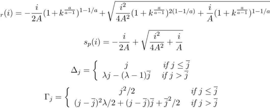
sr(i) =
i
2A(1 +k
a
a 1)1 1=a+
r i2
4A2(1 +k
a
a 1)2(1 1=a)+ i A(1 +k
a
a 1)1 1=a
sp(i) = i 2A +
r i2
4A2 + i A
j = j (j 1)j ififj > jj j
j =
j2=2 if j j
(j j)2 =2 + (j j)j+j2=2 if j > j
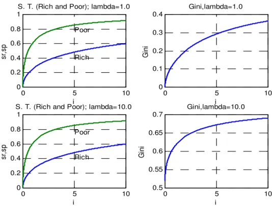
The value of the Gini coe¢cient for di¤erent values of the interest rate can be obtained using (21) and the above expressions. Table 1 presents the values of sr; sp and of the Gini coe¢cient for the parameter values a= 0:3,
A= 1,k= 0:25, j= 0:757; = 1 and interest rates equal to 0, 100%, 500% and 1000%.
Table 1, = 1
Interest Rate (%) 0 100 500 1000
sr 0 0.2579 0.4819 0.5993
sp 0 0.6180 0.8541 0.9161
Gini Coe¢cient (I) 0 0.1431 0.2921 0.3641
Figure 1 presents the evolution of the shopping time of rich and poor, as well as of the Gini coe¢cient, when interest rates assume values between zero and a thousand percent. The two upper graphs present the case in which
= 1 (as in Table 1), and the remaining graphs the case with = 10:
Some points are worth noting with regard to the data generated in this example. First, from equation (22), the value of the Gini coe¢cient when the interest rate is equal to zero reads:
I(0) = ( 1)j(1 j)
j+ (1 j) (23)
Table 1 has been constructed under the assumption that = 1; implying, by the above formula, that G(0) = 0; as one can read at the bottom of the second column of the table. In this case ( = 1);all inequality, which ranges from zero to 0:3641, is generated by in‡ation. Higher or lower values of the variables in Table 1 can be generated by allowing the parameterAto assume lower or higher values, respectively.
Figure 1 also includes the data when = 10: Note that the Gini coef-…cient is di¤erent from zero (its value is given by (23)) when the interest rate is equal to zero. Indeed, in this case we are assuming that a part of the population is more productive than the other, something which did not happen in the case = 1:
Note also that the shopping times of the rich and of the poor do not depend on :
5
In‡ation Tax and Shopping Time
So far, our theoretical analysis has focused solely on a shopping-time rea-soning in studying the link between in‡ation and inequality.
The purpose of this section is to show that in our formalization of the problem, shopping times of both the rich and the poor read as a constant times the in‡ation tax they pay. To express it di¤erently, our examination of inequality based on the shopping-time rationale can be understood as a mirror image of the usual in‡ation-tax argument that links in‡ation to inequality.
Indeed, for the sake of generality, make:
F(m; x; s) =G(m; x)s ; 0< 1
in (10). Note that can assume the value 1, used throughout the text, or another value less than one (see footnote 3 and also the discussion at the bottom of page 265, in Lucas (2000)). Under this speci…cation, equations (15) and (16) read, respectively:
and
sp = i mp (25)
Equation (24) shows that, in equilibrium, the fraction of time spent by the rich as shopping time is actually a constant ( ) times the in‡ation tax that they pay8: Equation (25) leads to the same conclusion, this time regarding the poor.
This point, namely that the welfare costs of in‡ation under the shopping-time rationale can be seen as a mirror image of the in‡ation tax, is not new in the literature. As we mentioned in the introduction, it has been noted by Lucas (1993, p. 14, eq. 4.14) and also appears in Lucas (2000, p. 266)9.
Equation (24) generalizes Lucas’s …nding for the case in which there is a second transacting balance in the economy.
The connection made by equations (24) and (25) adds a new dimension to our results here, by allowing a link between our approach to in‡ation and inequality, focusing solely on the shopping-time argument, and the more conventional argument, based on the di¤erentiated in‡ation tax paid by both rich and poor. It also connects our results to the empirical evidence concerning the usual in‡ation-tax argument.
6
Conclusions
We have developed a simpli…ed model, based on a shopping-time rationale, to investigate the e¤ect of in‡ation on the Gini coe¢cient of income distrib-ution. A basic assumption of the model is that some (cohorts of) consumers have access to a better transacting technology than others.
Our main conclusion is that under such assumptions a formal link be-tween in‡ation and the Gini coe¢cient of income distribution can be theo-retically proved. For transacting technologies in which the productivity of the interest-bearing asset is high enough, an increase of the in‡ation rate unequivocally leads to a deterioration of the income distribution. A link between our approach to the problem and the usual in‡ation-tax reasoning, which connects in‡ation to income inequality, has also been presented, as well as an example to illustrate our point.
8The argument actually refers to the opportunity cost of holding the transacting assets
m(given byi mr; p) andx(given by(i ix)xr), compared to holding bonds. But these are exactly the quantities to which the the usual argument linking in‡ation and inequality refers. See also footnote 2.
9A non-numbered equation in page 266 of Lucas (2000) is equal to equation (25), for
.
References
[1] Bulir, Ales, (2001): "Income Inequality: Does In‡ation Matter?" IMF Sta¤ Papers, Vol. 48, n. 1.
[2] Cysne, Rubens P. (2002): “On the Integrability of Partial Equilibrium Measures of the Welfare Costs of In‡ation.” Journal of Banking and Finance, 26, 12, 2357-2363.
[3] Cysne, Rubens P. (2003): ”Divisia Index, In‡ation and Welfare”. Jour-nal of Money, Credit and Banking, Vol. 35, 2, 221-239.
[4] Easterly, W. and Stanley Fischer (2001): "In‡ation and the Poor", Journal of Money, Credit and Banking, Vol. 33, N. 2, Part I, 160-178.
[5] Galli, R. and Hoeven, R. (2001): “Is in‡ation bad for income inequality? The importance of the initial rate of in‡ation”. Working Paper, The University of Lugano, Switzerland.
[6] Lucas, Robert E. Jr. (1993): “The Welfare Costs of In‡ation”. Univer-sity of Chicago working paper.
[7] _________, (2000): “In‡ation and Welfare.” Econometrica 68 62 (March 2000), 247-274.
[8] Mulligan, Casey B. and Xavier X. Sala-i-Martin, (1996): "Adoption of Financial Technologies: Implications for Money Demand and Monetary Policy", NBER Working Paper Series, n. 5504
[9] Romer, Christina D. and David H. Romer, (1998): "Monetary Policy and the Well-Being of the Poor", NBER Working Papers Series, n. 6793.
0 5 10 0
0.2 0.4 0.6 0.8 1
S. T. (Rich and Poor); lambda=1.0
i
sr
,sp
Poor
Rich
0 5 10
0 0.1 0.2 0.3 0.4
Gini,lambda=1.0
i
Gi
ni
0 5 10
0 0.2 0.4 0.6 0.8 1
S. T. (Rich and Poor); lambda=10.0
i
sr
,sp
Poor
Rich
0 5 10
0.5 0.55 0.6 0.65 0.7
Gini,lambda=10.0
i
Gi
ni