Linkage disequilibrium and genomic selection in pigs

RENATA VERONEZE

LINKAGE DISEQUILIBRIUM AND GENOMIC SELECTION IN PIGS

Thesis presented to the Breeding and Genetics Graduate Program of the Universidade Federal de Viçosa, in partial fulfillment of the requirements for degree of Doctor Scientiae.

VIÇOSA

Ficha catalográfica preparada pela Biblioteca Central da Universidade Federal de Viçosa - Câmpus Viçosa

T

Veroneze, Renata, 1984-V549l

2015

Linkage disequilibrium and genomic selection in pigs / Renata Veroneze. – Viçosa, MG, 2015.

xi, 145f. : il. ; 29 cm.

Orientador: Paulo Sávio Lopes.

Tese (doutorado) - Universidade Federal de Viçosa. Referências bibliográficas: f.134-145.

1. Suíno - Genética. 2. Genética quantitativa. 3. Marcadores genéticos. I. Universidade Federal de Viçosa. Departamento de Zootecnia. Programa de Pós-graduação em Genética e

Melhoramento. II. Título.

RENATA VERONEZE

LINKAGE DISEQUILIBRIUM AND GENOMIC SELECTION IN PIGS

Thesis presented to the Breeding and Genetics Graduate Program of the Universidade Federal de Viçosa, in partial fulfillment of the requirements for degree of Doctor Scientiae.

APROVADA: 25 de setembro de 2015.

Profa.Simone E. F. Guimarães (Coorientador)

Dr. Marco Antonio Machado

Dra. Mônica Corrêa Ledur Dr. Moyses Nascimento

ii

“I must endure the presence of two or three

caterpillars if I wish to become acquainted

with the butterflies”

iii ACKNOWLEDGEMENTS

Most of the gains we have achieved in our lives would not have been possible without the direct or indirect contributions of many hands. I feel myself a very lucky person because in this journey I had the opportunity to learn with a lot of people.

Paulo Sávio, I am grateful for you to be my advisor since the bachelor and for your guidance in science. I always admire your professionalism and rectitude. Thank you for the great professional experiences that would not have been possible without the support of you and Simone.

Simone, thank you for giving me lessons that extend beyond academia and for always making me believe in myself. Your strength and capacity to build scientific networks are admirable.

Fabyano, your enthusiasm for scientific research is amazing and contagious. Thank you, for all the great ideas, discussions and scripts. I am grateful for your friendship and for always trying to help me inside and outside the university.

Dear Johan, your scientific view enhanced my papers and this thesis . Thank you for your kindness and for your support in pursuing my PhD. Without your help with all the formalities and agreements the PhD at Wageningen University would not have been possible.

iv professor. Thank you for your dedication and for your invaluable help with this thesis.

Dear Egbert and Barbara thank you for challenging me to go deep into the practical and biological insights of my research. It helped me to improve the thesis and to broaden my scientific vision.

I feel really proud of being your friend Marcos! You have been taking such a successful and beautiful path. Thank you for our friendship, for the constructive help while working on this thesis.

André, thank you for your contribution to this thesis and our friendship.

Thanks to all members of ABGC. The time that I spent at WUR was short but rich because of all of you.

Ada and Lisette thank you for the fundamental help with all my documents. Lisette I am really grateful for your help in handling my thesis.

I would like to thank the Topigs Norsvin Research Center for the data and for all the support that they provided to my research.

Thank you to CNPq, FAPEMIG and CAPES for their financial support.

Thank you to the Universidade Federal de Viçosa and Graduate Program of Breeding and Genetics for the support and for making possible de PhD double-degree.

v André, Darlene, Vanessa, Carolina, Walmir, Rafael, Cândida and Luiz, the times that we had are unforgettable, mainly the funny ones. Thank you for making my life happier and easier. For being my partners in beers, barbecues and pizza.

Thank you Lucas, Katiene and Priscila for our scientific discussions and friendship.

Vanessa and Carolina thank you for the great times that we had in Wageningen.

Saturday is always the best day of the week because of MEIMEI. Thank you to all the members and kids of this institution.

My dear friend Thaís thanks a lot for all these years of friendship. Your advice is always a good guide.

Rosana and Junior, thank you for being my full-time friends and for us being always united even when apart.

vi BIOGRAPHY

Renata Veroneze was born on July 27th in Capivari, Brazil. She grew up on a farm in Elias Fausto, which was the inspiration to take the BSc in Animal Science. She began her studies in Animal Science at the Universidade Federal de Viçosa in 2004. In the beginning of her bachelor she became interested in genetics and statistics and in 2006 became a Junior researcher at the Animal Breeding group. During her bachelor she did an internship in the Netherlands at the Institute for Pig genetics and in January 2009 she graduated with a BSc in Animal Science. The following February, Renata started her MSc in Animal Science at Universidade Federal de Viçosa. In

February 2011, she defended her MSc thesis entitled: “Linkage

disequilibrium and haplotype block structure in six commercial pig lines”. In the same month, she started her PhD in Genetics and Breeding at Universidade Federal de Viçosa. The PhD project was built in a partnership with the Animal breeding and Genetic group of Universidade Federal de Viçosa, and the Animal Breeding and Genomics Centre of Wageningen University. Renata was accepted as a PhD candidate at the Animal Breeding and Genomics Center at Wageningen University in 2014. During her PhD,

she worked on the project “Linkage disequilibrium and genomic selection in

pigs”, and focused on the characterization of LD patterns in different pig

vii SUMMARY

viii RESUMO

VERONEZE, Renata, D.Sc., Universidade Federal de Viçosa, setembro de 2015. Desequilíbrio de ligação e seleção genômica em suínos. Orientador: Paulo Sávio Lopes. Coorientadores: Simone Eliza Facioni Guimarães e Fabyano Fonseca e Silva.

ix leva a hipotetizar que associações marcador-QTL similares poderiam ser encontradas em animais cruzados e as linhas parentais e, portanto, esperava-se encontrar altas acurácias de predição genômica entre essas populações. Entre as linhas puras a persistência de fase foi baixa, logo painéis de SNPs de maior densidade deveriam ser utilizados para manter a mesma associação marcador-QTL entre essas linhas. Acurácias obtidas na predição genômica utilizando animais cruzados assim como os arranjos across e multi, não seguiram as expectativas baseadas em LD. Portanto, a

consistência de fase de ligação entre populações pode não ser tão importante para a acurácia da seleção genômica como se pensava, mas sim a ação combinada de LD, arquitetura genética e frequências alélicas. Portanto, foi desenvolvida uma metodologia que leva em consideração differenças nas frequências alélicas, bem como informações dos GWAS para comtemplar a arquitetura genética da característica. Esta estratégia trouxe alguns benefícios para a predição genônima para os arranjos within e multi. Ponderações obtidas por meio de GWAS em diferentes conjuntos de

x ABSTRACT

VERONEZE, Renata, D.Sc., Universidade Federal de Viçosa, September 2015. Linkage disequilibrium and genomic selection in pigs. Adviser: Paulo Sávio Lopes. Co-Advisers: Simone Eliza Facioni Guimarães and Fabyano Fonseca e Silva.

1

1

2 1.1 Introduction

Genomic selection was first applied to Holstein cattle, but currently, most major breeding companies have implemented it. Although genomic selection is used in practice, its application presents some challenges. Several knowledge gaps remain to be bridged to enable the creation of practical, feasible methods for applying this new technology. Many aspects of quantitative and population genetics are revisited in the context of genomic selection. In this thesis, I report my research on linkage disequilibrium and on practical strategies and methods for the implementation of genomic selection in pigs.

1.2 Linkage Disequilibrium

Linkage disequilibrium (LD) is a non-random association between alleles at different loci (Ardlie et al., 2002). These allelic associations are mainly due to physical proximity, but they are also influenced by population history and evolutionary forces (Khatkar et al., 2008). For example, the extent of LD depends on local recombination rates. Therefore, the LD is higher in regions with low recombination rates, which for mammals, includes the Y chromosome, parts of the X chromosome, and regions near the centromere in autosomes. Conversely, the LD is lower in regions with high recombination rates, such as euchromatin and small regions known as hotspots (Jeffreys et al., 2001).

3 cause gene-frequency evolution can lead to differences in the LD of specific genomic regions (Slatkin, 2008).

Genomic selection and genome wide association studies (GWAS) rely on the LD between DNA markers and quantitative trait loci (QTL) to estimate genomic breeding values (GEBV) or to detect regions that control traits of interest. In evaluating how efficiently GWAS results were transferred across people of European and East Asian ancestries, Marigorta and Navarro (2013) suggested that a proportion of the associations found in Europeans failed to replicate in East Asians, due to the heterogeneity in LD between causal variants and tag-SNPs. In genomic selection, it has been shown that the GEBV accuracy depends at least partly on the LD between the DNA markers and the QTL (Hayes et al., 2009).

The LD in commercial pig populations extends over larger distances than in cattle. The currently, widely-used pig SNP panel (Porcine SNP60, Illumina Inc, San Diego, USA) appears to have an adequate number of DNA markers to provide a sufficient level of LD for effective GWAS and genomic selection (Uimari and Tapio, 2011; Badke et al., 2012; Veroneze et al., 2013; Wang et al., 2013). This high level of LD also benefits the imputation of SNP genotypes (Pei et al., 2008) and opens the possibility of using low density panels in pigs.

4 populations. An inconsistent LD phase can explain why a marker associated with an important effect in one population may not be effective for selection in a second population.

Badke et al. (2012) evaluated the Landrace, Yorkshire, Hampshire, and Duroc pig breeds. They found that the correlations of LD phase ranged from 0.87, between Duroc and Yorkshire pigs, to 0.92, between Landrace and Yorkshire pigs, for markers with a pairwise distance <10 Kb. For markers separated by the same distances, Wang et al. (2013) found a somewhat lower persistence of phase, with correlations of 0.61 between Duroc and Landrace, 0.57 between Duroc and Yorkshire, and 0.66 between Landrace and Yorkshire pigs. Therefore, the current 60K pig marker panel may have insufficient density to maintain LD phase consistency across all pig breeds.

1.3 Modeling for linkage disequilibrium prediction

Linkage disequilibrium can be computed for each pair of loci in the genotype dataset; this procedure can generate a large amount of output data. Summarizing the data provides better comprehension of the LD patterns in different populations. To date, the relationship of LD to the physical distance between markers (LD decay) has been studied, either by calculating simple averages within predefined windows of distance (Uimari and Tapio, 2011; Badke et al., 2012; García-Gámez et al., 2012; Veroneze et al., 2013) or using parametric nonlinear regression models (Heifetz et al., 2005; Amaral et al., 2008; Abasht et al., 2009).

5 recombination (Sved, 2009). The model derivation assumed that the population was isolated, mating was random, and the population size remained constant over time. These assumptions are likely to be violated in most natural and selective breeding populations. Moreover, nonlinear regression models generally assume that errors are independent, have homogeneous variance, and are normally distributed. These assumptions are violated, due to the nature of LD data, which is dependent on the distance between markers and is more variable at short distances than at long distances. Consequently, some alternatives have been proposed for modeling LD decay. Instead of using a fixed value of unity for the intercept, Corbin et al. (2010) introduced a new parameter to estimate the intercept in the equation proposed by Sved (1971); this new parameter may provide a better fit to the LD at short distances. LOESS regression is also a good option for describing the LD decay, because it allows the functional form between dependent and independent variables to be determined by the data without requiring strong assumptions (Andersen, 2009).

1.4 Genomic selection in pigs

6 reducing the generation interval. Therefore, the most important advantage of genomic selection in pig breeding is the increased accuracy it can provide. The accuracy of GEBV depends on several factors, including the LD between the markers and the QTL, the number of animals in the reference population, the heritability of the trait, the distribution of QTL effects (Hayes et al., 2009), and the level of family relationship between the reference population and the selection candidates (Wientjes et al., 2013).

The implementation of genomic selection in pigs is more complicated than in cattle, due to the characteristics of pig breeding. Pig breeding is a pyramidal system, with a small nucleus population and short generation intervals; also, it is typically guided by diverse breeding goals (Ibáñez-Escriche et al., 2014). The small population size complicates the implementation of highly accurate genomic selection, because the accuracy of the GEBV depends on the size of the reference set. The short generation interval inherent in pig breeding removes an important benefit of genomic selection, compared to the situation in cattle. Due to the fact that more generations are produced per unit of time, pig breeding requires frequent re-estimations of marker effects. In addition, the reduction in family relationships will be accelerated. The lack of family relationships between reference and prediction animals will reduce the accuracy of GEBV.

1.5 Across- and multi-population genomic selection

7 multiple lines in a breeding program, that each are of limited size, may however point to a solution for increasing accuracies. The size of the reference population for a given line could be doubled, or more, by using data from other lines in multi- or across-population genomic selection and with the use of crossbred information.

The use of multi- and across-population reference sets has been tested in simulation studies (Ibánez-Escriche et al., 2009; Toosi et al., 2010; Zeng et al., 2013) and in real data in cattle (Hayes et al., 2009), sheep (Legarra et al., 2014), pigs (Hidalgo et al., 2015), and chickens (Simeone et al., 2012). Simulation studies have indicated that favorable effects on accuracy could be achieved mainly by using multiple populations. In contrast, studies that use real data have shown both positive and negative outcomes. In a simulation study, de Roos et al. (2009) evaluated the effects of combining multiple populations on the accuracy of genomic selection. Those authors concluded that the greatest benefits of combining populations were achieved when the populations had diverged for only few generations, the marker density was high, and the heritability was low.

8 (2012) concluded that the breeds with small reference sets gained the most GEBV accuracy by using a reference set that comprised multiple breeds. On the other hand, Legarra et al. (2014) evaluated genomic predictions for six breeds of sheep, and they concluded that the use of multiple populations only marginally increased the accuracy, and only for a few breeds.

A common outcome of those studies was that the relationships between breeds had an important influence on the accuracy of the GEBV, when using multi- or across-population reference sets. These multi- and across population approaches may provide promising opportunities for genomic prediction in the pig industry, where some lines share a common genetic background. Moreover, the pig industry aims to improve the performance of crossbred animals. Therefore, data from crossbreds could provide powerful additional information to the reference population, because the crossbreds are closely related to purebred candidates.

1.6 Aim and outline of this thesis

11

2

Linkage disequilibrium patterns and

persistence of phase in purebred and

crossbred pig (

Sus scrofa

_{) populations}

12 Abstract

Genomic selection and genomic wide association studies are widely used methods that aim to exploit the linkage disequilibrium (LD) between markers and quantitative trait loci (QTL). Securing a sufficiently large set of genotypes and phenotypes can be a limiting factor that may be overcome by combining data from multiple breeds or using crossbred information. However, the estimated effect of a marker in one breed or a crossbred can only be useful for the selection of animals in another breed if there is a correspondence of the phase between the marker and the QTL across breeds. Using data of five pure pig (Sus scrofa) lines (SL1, SL2, SL3, DL1, DL2), one F1 cross (DLF1)

and two commercial finishing crosses (TER1 and TER2), the objectives of this study were: (i) to compare the equality of LD decay curves of different pig populations; and (ii) to evaluate the persistence of the LD phase across lines or final crosses.

13 This study showed that crossbred populations could be very useful as a reference for the selection of pure lines by means of the available SNP chip panel. Here, we also pinpoint pure lines that could be combined in a multiline training population. However, if multiline reference populations are used for genomic selection, the required density of SNP panels should be higher compared with a single breed reference population.

Key words: nonlinear model, single nucleotide polymorphism, SNP, genomic selection

2.1 Introduction

Linkage disequilibrium (LD) is a nonrandom association between alleles at different loci (Ardlie et al., 2002). There has been a growing interest in LD analysis with the explosion of genomic selection (GS) and genome wide association studies (GWAS) published in recent years. Both GS and GWAS exploit the LD between markers and quantitative trait loci (QTL) to estimate genomic breeding values (GEBV) or to detect regions that control traits of interest.

14 combining animals from different breeds or lines (Hayes et al., 2009b). Daetwyler et al. (2012) showed that GEBV are more accurate than pedigree-based best linear unbiased prediction (BLUP) using a multibreed sheep training population.

Another approach that can be used to acquire a larger reference population is the inclusion of crossbred animal information, because large populations are available in commercial farms. Using crossbreds has several advantages: one crossbred population could be used to select more than one pure line, the phenotypes of production animals can be more relevant for breeders and the animals can be selected for traits that are not measured in the nucleus herd (e.g. disease resistance). In addition, using crossbred data it may be possible to account for heterotic effects in the selection. Using marker information, Amuzu-Aweh et al. (2014) showed that it was possible to identify specific sires whose offspring could be expected to show higher levels of heterosis. These approaches are especially attractive for the pig industry, where breeding companies keep a range of sire and dam lines. Using crossbred reference populations could reduce the need to establish separate large reference populations for each pure line.

15 2002). GS uses direct relationships and LD to predict breeding values. When predictions are carried out in populations with distantly related individuals, the accuracy is mainly determined by LD between markers and QTL, while predictions with closely related individuals rely mainly on direct relationships (Daetwyler et al., 2012). Thus, when the relatedness across breeds is small, the accuracy of prediction is mainly reflected in the LD between markers and QTL. In addition, knowledge of the persistence of phase across physical distance between markers for two populations can be used to determine which marker density is needed to provide the same LD phase across these populations (de Roos et al., 2008).

Badke et al. (2012), when evaluating the Landrace, Yorkshire, Hampshire and Duroc breeds, found that the correlation of phase ranged between 0.87 for Duroc-Yorkshire and 0.92 for Landrace-Yorkshire, for markers with a pairwise distance <10 Kb. While, for the same distance, Wang et al. (2013a) found a persistence of phase of 0.61 for Landrace, 0.57 for Duroc-Yorkshire and 0.66 for Landrace-Duroc-Yorkshire. Studies evaluating LD and persistence of phase in crossbred pig lines are scarce, and the comparison of LD decay in different populations has been achieved visually using average LD (de Roos et al., 2008; Uimari and Tapio, 2011; Badke et al., 2012; Veroneze et al., 2013; Wang et al., 2013a), without the application of models or statistical comparisons.

In the present study, we evaluated five pig pure lines (SL1, SL2, SL3, DL1, DL2), one F1 cross (DLF1) and two commercial finishing crosses (TER1 and

16 of different populations; and (ii) to evaluate the persistence of phase across populations.

2.2 Methods

This experiment was conducted strictly in line with the Dutch law on the protection of animals.

2.2.1 Data

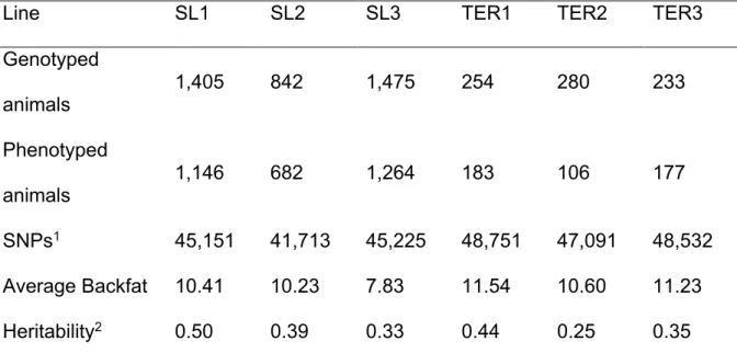
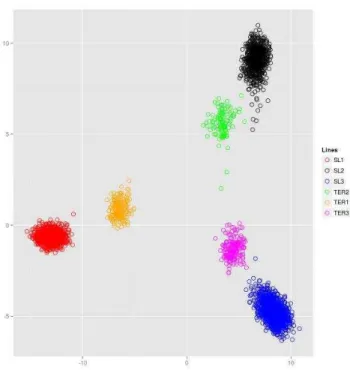
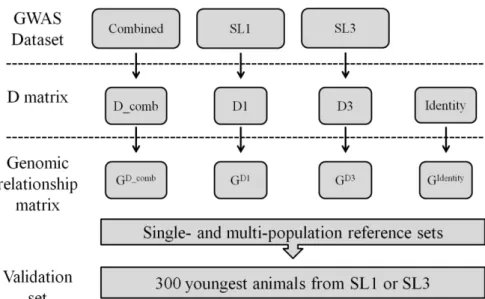
The data for this study were obtained from animals from five pig pure lines (SL1, n=1,307; SL2, n=643; SL3, n=276; DL1, n=626; DL2, n=1013), one F1 cross (DLF1, n=186) and two commercial finishing crosses (TER1, n=286; TER2, n=330). SL1 and SL2 are synthetic sire lines; SL1 is a combination of Duroc (mostly) and Belgian Landrace created in about 1980. SL2 is a combination of Large White and Pietrain created in about 1975. SL3 is a Pietrain sire line. DL1 is Landrace based dam line and DL2 is a Large White based dam line. DLF1 is a commercial F1 cross resulting from crossing animals of DL1 and DL2. TER1 is a commercial finishing pig resulting from a cross between DLF1 and SL1. TER2 is also a commercial finishing pig that resulted from a cross between DLF1 and SL2. All pure lines were kept under strict inbreeding restrictions, with approximately 40 replacement sires per year and more than 250 gilt replacements per year.

17 chromosome would show higher LD than the overall genome (Schaffner, 2004), which could cause an overestimation of the LD. The R software (http://www.r-project.org/) was used for within population marker quality control, using the package GenABLE (Aulchenko et al., 2007). Markers with a call rate <90%, MAF <0.05 and/or a p-value for the Hardy-Weinberg equilibrium <0.0001 were excluded. The summary of the quality control of genotype data is presented in supplementary material (Table S2).

To estimate the persistence of phase, the data were divided into four groups, according the description shown in supplementary material (Table S2), and only SNPs that passed the quality control in all lines of each group were used. In group 1, the F1 (DLF1) cross was compared with its parental lines, while in groups 2 and 3 the finishing crosses (TER1 and TER2) were compared with their parental and grandparental lines. In group 4, which included only pure lines, each line was compared with all other pure lines.

2.2.2 LD

For each pig line, the LD between SNPs was computed as the correlation of

gene frequencies ( 2 ij

r ) (Hill and Robertson, 1968) using the function LD of the

package genetics (Warnes and Leisch, 2005) of the software R (http://www.r-project.org/):













where pi and pj are the marginal allelic frequencies at the th

18 estimated using maximum likelihood because genotype data were used (Warnes and Leisch, 2005).

2.2.3 LD decay

Decay of LD with the distance between markers was compared between lines. Only SNPs that passed the quality control filtering in all lines were used in this analysis. The comparison was conducted by adjusting the nonlinear regression model proposed by Sved (1971) to allow for testing a curve equality hypothesis (Bates and Watts, 1988) across the eight populations evaluated. For the curve equality test, the nonlinear model receives a dummy variable that represents each one of the eight populations. This complete model is described as:

, e d 4 1 1 D LD ik i k 8 1 k k

ik 

       



LD

r for marker pair iof line k;

:

such that

able,

dummy vari

an

is

D

Dk ik

i

d is the distance in Kb for marker pair i;

k

 is the coefficient that describes the decline of LD with distance for line k;

ik

e

 

19 k k ) 1 ( a k ) 1 (

0 : k vsH : for at least one

H     

To test the (1) 0

H hypothesis, the following comparison scheme was conducted,

considering the complete (1) and the reduced (2) models:

, e d 4 1 1 D LD ik i 8 1 k k

ik 

       



where a single parameter for all lines is assumed.

The residual sum of squares of the complete (

SQR

models are used to perform a chi-squared statistic:







2computed Nln SQR SQR , in which Nis the number of observed measures

of LD. The hypothesis (1) 0

H is rejected if 2_{ } v 2

computed

 , where vp_ p_is the

degree of freedom, where

p

complete and reduced models, respectively, at a significance level .

Rejection of the hypothesis (1) 0

H implied that at least one parameter  differs

from the others, and, subsequently, a pairwise comparison was carried out to identify the lines that are equal or different in relation to the parameter .

Multiple tests were carried out; therefore, the Bonferroni correction was employed to reduce Type I errors. In this case, the significance threshold (

*

 ) was obtained by dividing the established significance threshold for a

single test (0.05) by the number of independent tests (n). Thus, for the present study, the significance level for pairwise comparison was

20 The nonlinear models were adjusted using the function nls of the software R (http://www.r-project.org/), and the hypothesis tests were also conducted using R scripts.

2.2.4 Persistence of phase

The squared root of 2 ij

r was obtained and given the same sign as D, which

was calculated as described by de Roos et al. (2008), using the R software (http://www.r-project.org/).







22

f

f

f

f

f

D









where:





22B A B A B

A

22 2p p p

f





11B A B A B

A

12 2p p p

f





22B A B A B

A

21 2p p p

f 12 12B A p 2 2   where 12 12B A

p is the proportion of animals with heterozygous genotypes at both

loci.

This approach was first described by Goddard et al. (2006), and the setting of the D sign was conducted to consistently define the statistic in all lines. The

2 ij

r received the same sign in two breeds if the same haplotype was more

common than expected from the allele frequencies in both breeds.

To express the correlation of 2 ij

r across populations in relation to the physical

distances between SNPs, the Pearson correlations between 2 ij

r values were

21 of 50 kb was chosen based on the coefficient of variation (CV) of the number of SNP pairs for intervals of 10, 30, 50, 70 and 100 kb [see supplementary material: Table S2] to guarantee that the most similar number of observations in each bin were used to calculate the correlation. Based on the CV evaluation, there was no evidence of difference in the use of bins of 30, 50, 70 and 100 kb; thus the value of 50 Kb was chosen to give a more detailed LD description in relation to the bins of 70 and 100 kb, and a better visualization in relation to the bin of 30 kb.

2.3 Results

2.3.1 LD decay

The nonlinear model for the decay of LD with distance was adjusted to

simultaneously describe multiple lines. The model parameter kdescribes

the decline of LD with distance for each line. The estimates of ˆkranged from

1.25×10−3 _{to 2.92×10}−3 _{and were all significantly different from zero (p-value}

22 Table 2.1 Parameter estimate (ˆk), standard error and p-value for the nonlinear fitted model for each line.

Line ˆk Std. Error p-value

SL1 1.78×10−3 _4.76×10−6 _<10−3

SL2 1.25×10−3 _2.89×10−6 _<10−3

SL3 1.69×10−3 _4.42×10−6 _<10−3

DL1 2.12×10−3 _6.09×10−6 _<10−3

DL2 1.71×10−3 _4.49×10−6 _<10−3

DLF1 2.44×10−3 _7.46×10−6 _<10−3

TER1 2.92×10−3 _9.63×10−6 _<10−3

TER2 2.03×10−3 _5.75×10−6 _<10−3

The adjusted model to describe the LD permits a statistical comparison of the lines with respect to the decline of LD with distance, which is important to infer the size of single nucleotide polymorphism (SNP) panels for GS and GWAS in these lines. To compare the lines, the equality of the LD curves

was tested. The first hypothesis tested (H : k k

) 1 (

0   ) states that the model to describe the LD decay is the same for all lines. This hypothesis was rejected (p-value <10−3), which implies that at least one parameter β differs

from the other parameters. Next, a pairwise comparison was carried out that aimed to identify which lines are equal or different regarding the parameter 

. All pairwise comparisons were significantly different [see supplementary

material: Table S2], with the exception of the comparison between _SL3and

2 DL



23 these two lines. In addition, SL2 showed the smallest  value, which implied

that this line has the largest extent of LD, while TER1 showed the largest 

value and consequently the shortest LD.

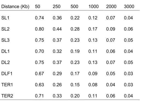
The test of the equality of the LD decay curves showed that the overall pattern of LD decay differed between lines. The predicted LD was reported at specific marker distances (Table 2.2), with the highest values of predicted LD observed for SL2 at various distances, while TER1 presented the lowest values. SL3 and DL2 presented the same values of predicted LD, because

the β parameters of these lines did not differ statistically. All lines presented

low values of LD for marker distances above 3000 kb. At these large marker distances, the crossbreds exhibited similar levels of LD compared with the pure lines.

Table 2.2 Predicted r² at various distances (Kb) for eight pig populations.

Distance (Kb) 50 250 500 1000 2000 3000

SL1 0.74 0.36 0.22 0.12 0.07 0.04

SL2 0.80 0.44 0.28 0.17 0.09 0.06

SL3 0.75 0.37 0.23 0.13 0.07 0.05

DL1 0.70 0.32 0.19 0.11 0.06 0.04

DL2 0.75 0.37 0.23 0.13 0.07 0.05

DLF1 0.67 0.29 0.17 0.09 0.05 0.03

TER1 0.63 0.26 0.15 0.08 0.04 0.03

25 Table 2.3 Average and standard deviation r² at various distances (Kb) for eight pig populations.

Dist 0–50 200–250 500–550 1000–1050 2000–2050 3000–3050

SL1 0.49 ± 0.37 0.30 ± 0.31 0.23 ± 0.27 0.18 ± 0.23 0.12 ± 0.19 0.10 ± 0.16

SL2 0.55 ± 0.37 0.35 ± 0.33 0.28 ± 0.30 0.21 ± 0.25 0.14 ± 0.21 0.11 ± 0.18

SL3 0.50 ± 0.37 0.29 ± 0.30 0.24 ± 0.27 0.18 ± 0.23 0.13 ± 0.19 0.10 ± 0.17

DL1 0.49 ± 0.36 0.29 ± 0.30 0.21 ± 0.26 0.16 ± 0.22 0.11 ± 0.18 0.09 ± 0.16

DL2 0.51 ± 0.37 0.31 ± 0.31 0.24 ± 0.27 0.18 ± 0.24 0.12 ± 0.19 0.09 ± 0.16

DLF1 0.47 ± 0.36 0.27 ± 0.29 0.20 ± 0.24 0.15 ± 0.21 0.10 ± 0.16 0.08 ± 0.14

TER1 0.46 ± 0.35 0.25 ± 0.28 0.18 ± 0.23 0.14 ± 0.19 0.09 ± 0.15 0.07 ± 0.13

26 2.3.2 Persistence of linkage disequilibrium phase

In pig production, crossbred animals are used for reproduction on commercial farms. The line DLF1 represents these crossbred females, and crossing the dam lines DL1 and DL2 produces these animals. DLF1 presented a similar LD compared with lines DL1 and DL2, with high persistence of phase, a correlation of >0.9 for marker distances up to 150 Kb and a correlation of >0.8 for marker distances up to 1200 Kb (Figure 2.1a). Commercial finishing pigs TER1 and TER2 are the end product of the pig industry, and are based on a cross between DLF1 and either SL1 or SL2, respectively. TER1 showed higher persistence of phase with SL1 and DLF1 compared with lines DL1 and DL2 (Figure 2.1b); this result was expected because the haplotype sharing is different between TER1 and these four populations. TER1 showed a correlation of phase of >0.9 for markers at distances below 200 Kb in relation to lines SL1, DLF1, DL1 and DL2 (Figure 2.1b).

Similar to TER1, TER2 showed greater persistence of phase with SL2 and DLF1 compared with lines DL1 and DL2 (Figure 2.1c). The distance at which the correlation of phase remained >0.9 was higher for TER2 compared with TER1, with distances of 1050 Kb, 400 Kb, 150 Kb and 50 Kb in relation to the lines SL2, DLF1, DL1 and DL2, respectively (Figure 2.1c).

27 different lines. SL1 and DL1 have contributions from the Landrace breed, while SL2 and DL2 have contributions from the Large White breed.

28 Figure 2.1 Correlation of phase (rij_{) in relation to the distance. a. Correlation}

between F1 (DLF1) and its parental lines (DL1 and DL2). b. Correlation between terminal cross (TER1) and its (grand)parental lines (SL1, DLF1, DL1 and DL2). c. Correlation between terminal cross (TER2) and its (grand)parental lines (SL2, DLF1, DL1 and DL2). d. Correlation across all pure lines (SL1, SL2, SL3, DL1, DL2).

2.4 Discussion

29 especially for short distances below 50 kb. The persistence of LD between crossbreds and their (grand)parental lines followed the expectations based on the contributions that the different breeds made to each of the lines.

2.4.1 Equality of LD curves

A formal comparison of the level of LD decay was made possible by our adjustments to the nonlinear model described by Sved (1971). All of the lines studied followed the same pattern of a rapid decrease in LD as the distance increased. Previous comparisons of LD decay between breeds or lines was performed using average r² in distance bins (de Roos et al., 2008; Uimari and Tapio, 2011; Badke et al., 2012; Veroneze et al., 2013) and/or adjusting a linear model to test the breed effect (Amaral et al., 2008; Megens et al., 2009). The equality of curves test permits not only the identification of the existence of line differences, but also allows for a pairwise comparison across all lines. The test revealed that six of the eight evaluated lines differ

with respect to LD decay. Only the comparison between ˆSL3and ˆDL2was

30 be used for GS and GWAS for these lines, which could also influence the accuracy of GS.

2.4.2 LD in crossbreds

According to Reich et al. (2001), the extent of LD depends on the number of generations that have passed since the occurrence of an LD-generating event. In crossbred populations, LD comprises the existing LD in the parent populations and new LD generated in the cross as a result of different allele frequencies in the parental breeds (Toosi et al., 2010). The average LD for markers at distances up to 50 kb ranged from 0.47 to 0.50 in crossbreds and from 0.49 to 0.55 in the pure lines, while for markers at distances between 3000 and 3050 Kb, the LD ranged from 0.07 to 0.08 in crossbreds and from 0.09 to 0.11 in the pure lines. Surprisingly, the LD over large distances was not higher in crossbreds. A possible explanation for these similar LD levels in crossbred and pure lines may be the similarities in allele frequencies, or in LD phase, between the (grand)parental lines of the crossbreds. With similar frequencies, limited LD is created because of crossing (Toosi et al., 2010). Similarity in the allele frequencies could be caused by the fact that the minor allele frequency (MAF) was one of the criteria used to select markers for the 60K beadchip, which may have reduced the differences in allele frequency across lines (Ramos et al., 2009).

2.4.3 LD in pigs from the literature

31 and these results are similar to our findings for DL1 (Landrace based line) and DL2 (Large White based line). In addition, Uimari and Tapio (2011) reported r² values of 0.09 and 0.12 for SNPs that were 5 Mb apart in Finnish Landrace and Finnish Yorkshire pigs, respectively, which is higher than the average r² of 0.06 for DL1 and DL2 found in the present study.

By studying Duroc, Hampshire, Landrace and Large White from the USA, Badke et al. (2012) detected average r² values of 0.26, 0.25, 0.19 and 0.21 for SNPs that were 500 Kb apart, respectively, while in the present work, the lines SL1 (a combination of Duroc and Belgian Landrace), DL1 and DL2 presented average LDs of 0.23, 0.21 and 0.24, respectively. The differences regarding Duroc and SL1 could be explained by the breed composition of SL1, which contains Landrace genes, while differences in population structure, such as inbreeding and effective population size, could explain the LD differences of the Landrace and Large White breeds evaluated by Badke et al.(2012) and between DL1 and DL2. At large distances (5 Mb), the LD levels were similar to those found by Badke et al. (2012).

32 domestic breeds. Evaluating the LD of Chinese and Western pigs, Ai et al. (2013) found that Chinese breeds have lower extents of LD than Western pigs.

2.4.4 Implications for GS

An average LD greater than 0.2 has been reported to be required for GS (Meuwissen et al., 2001), and this LD level was observed for most of the evaluated lines at marker distances between 500 and 550 kb. All lines exhibited an average r² higher than 0.3 for markers 100–150 kb apart. Qanbari et al. (2010) found an average r² = 0.30 for markers at distances <25 kb for German Holstein cattle, and Bohmanova et al. (2010) found r² >0.3 for markers at distances of 60 kb in American Holstein cattle. Thus, in agreement with Veroneze et al. (2013) and Badke et al. (2012), it seems that LD extends further in European commercial pig breeds than in Holstein cattle, which implies that the use of less dense SNP panels is possible for GWAS and GS in pigs. Evaluating the use of low density panels associated with genotype imputation in pig sire lines, Wellmann et al. (2013) recommended that a panel with 384 markers could be used for genotyping selection candidates if at least one parent was genotyped at high-density. However, if multibreed reference populations are used for GS, the required density of SNP panels should be higher compared with a single breed reference population.

33 commercial pig populations, thus representing the crossbreeding structure of pig production design.

The high persistence of phase for SNPs with a 150 Kb distance when comparing DLF1, DL1 and DL2 implies that similar marker effects may be expected across the evaluated lines. The available porcine SNP chip should be dense enough to include markers that have the same LD phase with QTL across DLF1, DL1 and DL2. The persistence of phase with DLF1 shows the potential use of an F1 commercial cross as a reference population to select purebred lines. However, using pig purebreds to predict crossbred performance, Hidalgo (personal communication) found that the accuracies of the breeding values are trait-dependent, which challenges the use of the crossbred information in breeding programs.

34 Using crossbred animals in the reference population is expected to have a number of advantages. First, the utilization of crossbred performance to select purebreds enables selection for traits that cannot be measured at nucleus farms, such as disease resistance (Ibánez-Escriche et al., 2009). Second, a crossbred reference population may allow for reduced costs of GS when the same crossbred performance can be used as information for selection in two or more pure lines. Third, the use of crossbreds permits exploitation of the heterotic effects, which cannot be done when the selection is performed exclusively in purebreds. However, for the use of crossbred information, pig breeding programs need to adapt their data collection to obtain the phenotypes of F1 sows and finishing pigs, which can be challenging, because these animals are held on commercial farms.

2.4.5 Interpretation of the correlations between lines

35 SL2 and DLF1. Our assumption was that the higher persistence of phase of TER2 with its paternal line SL2 is caused by the higher LD observed in SL2. With the marker density provided by the pig 60K SNP panel, the data from TER1 could be used in GS strategies for SL1. Similarly, the data from TER2 could be used to select in SL2. The 60K SNP panel provides a marker density that shows a high persistence of LD phase between these lines. A much higher marker density would be necessary to ensure a persistence of phase between the lines TER1 and TER2 and between the dam lines DL1 and DL2.

While the correlations between crossbreds and their parental lines should allow for GS with a crossbred reference population using the SNP60Beadchip, the question remains whether the correlation of phase between pure lines is also high enough for a multibreed reference population design. The persistence of phase between pure lines depends on the time since their divergence took place (de Roos et al., 2008); i.e., the consistency of LD is directly related to the degree of relationship between lines (Andreescu et al., 2007). The highest persistence of phase was observed between SL2 vs. SL3 and SL2 vs. DL2. As described in the material and methods section, SL2 is a synthetic line resulting from the combination of the Large White and Pietrain breeds. SL3 is a Pietrain pure sire line and DL2 is a Large White pure dam line. Thus, the higher persistence of phase observed between SL2 vs. SL3 and SL2 vs. DL2 could be explained by the common breeds in the composition of these lines.

36 was found between the breeds Landrace and Large White for markers at distances of 10 kb, which is similar to the correlation observed between the lines DL1 and DL2 (which are Landrace- and Large White-derived lines, respectively) for markers at the same distance (0.93). The persistences of phase between SL1 vs. DL1 and SL1 vs. DL2 were higher (0.92 and 0.90, respectively) than the values found by Badke et al. (2012) between Duroc vs. Large White and Duroc vs. Landrace (0.87 for both) for markers at distances of 10 kb. Some difference was expected, because SL1 is a synthetic line of Duroc (mostly) and Landrace, so the highest persistence of phase in relation to the study of Badke et al. (2012) could be caused by the presence of the Landrace breed in SL1.

The lowest correlations of phase were observed between all lines and SL1. By evaluating the persistence of phase in Landrace, Large White and Duroc, Wang et al. (2013b) found a closer relationship between Landrace and Yorkshire and a more distant relationship between Duroc and Landrace/Large. By studying genetic diversity in native and commercial pig breeds in Portugal, including Duroc, Landrace, Large White and Pietrain, Vicente et al. (2008) concluded that Duroc is the more distant breed relative to the others. This could explain why the lowest correlations were observed between SL1 and the other lines.

37 SL2 and SL3 or SL2 and DL2, which presented the highest correlation of phase across the pure lines (>0.9 for markers at distances up to 50 Kb). The utilization of multibreed reference panels has been studied as a method to increase the reference population size (de Roos et al., 2008; Hayes et al., 2009; Daetwyler et al., 2012). Hayes et al. (Hayes et al., 2009) indicated that multi-breed reference populations will be a valuable resource to fine mapping of QTL. de Roos et al. (2008) concluded that multi-breed reference panels could increase the reliability of the GEBV when at least some animals of the target breed are included, and the benefit of combining populations increased when the populations have diverged for fewer generations. In addition, Daetwyler et al. (2012) showed that GEBV are more accurate than pedigree-based BLUP, using a multibreed sheep training population. According to Daetwyler et al. (2012), across breed accuracy depends on the LD between markers and QTL because the impact of the relatedness between the breeds is expected to be minimal. Thus, persistence of phase studies provide information for shaping multibreed, or in the case of the pig industry, multiline reference panels. Knowing the persistence of phase allows us to identify the lines that have diverged more recently and would provide higher relationship between reference and validation populations, a factor that plays a large role in the accuracy of the predictions.

2.5 Conclusions

39 Additional files

Additional file 1. Supplementary tables.

Table S1. Values of 2 computed



(below the diagonal) and p-values for the pairwise comparison

�̂_� �̂_� �̂ _� �̂ _� �̂ _� �̂ _� �̂ �̂

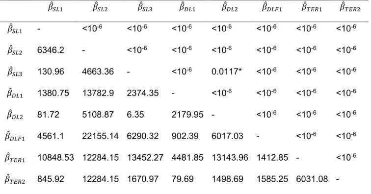
�̂� - <10-6 <10-6 <10-6 <10-6 <10-6 <10-6 <10-6

�̂� 6346.2 - <10-6 <10-6 <10-6 <10-6 <10-6 <10-6

�̂� 130.96 4663.36 - <10-6 0.0117* <10-6 <10-6 <10-6

�̂ � 1380.75 13782.9 2374.35 - <10-6 <10-6 <10-6 <10-6

�̂ � 81.72 5108.87 6.35 2179.95 - <10-6 <10-6 <10-6

�̂ � 4561.1 22155.14 6290.32 902.39 6017.03 - <10-6 <10-6

�̂ 10848.53 12284.15 13452.27 4481.85 13143.96 1412.85 - <10-6

�̂ 845.92 12284.15 1670.97 79.69 1498.69 1585.25 6031.08 -

40 Table S2. SNP data description according to the quality control criteria

SL1 SL2 SL3 DL1 DL2 DLF1 TER1 TER2

41 Table S3. Grouping of lines and the number of SNPs for persistence of phase estimation

Lines Group 1 Group 2 Group 3 Group 4

DL1 X X X X

DL2 X X X X

SL1 X X

SL2 X X

SL3 X

DLF1 X X X

TER1 X

TER2 X

42 Table S4. Coefficient of variation (CV) for the number of SNP pairs in bins of 10, 30, 50, 70 and 100 Kb

Distance intervals (Kb)

Group1 Group2 Group3 Group4

10 0.066 0.078 0.077 0.075

30 0.056 0.068 0.067 0.064

50 0.055 0.068 0.066 0.063

70 0.055 0.067 0.066 0.063

43

3

Comparison of nonlinear and loess regression

models for prediction of linkage disequilibrium

decay curves

44 Abstract

Knowledge about the relationship between linkage disequilibrium (LD) and physical distance can be used to infer the number of markers required to achieve a certain level of LD, which is useful for customization of SNP chips. Nonlinear and loess regression can be used to describe the relationship of LD with physical distance between markers; however, the impact of the regression models on LD predictions has not been investigated. Moreover, comparison of LD decay between different populations has been performed empirically without the application of a hypothesis test to determine whether curves differ significantly. Thus, proposals of comparison tests arise as a relevant point to be exploited in the field of statistical genomics. The objective of this study was to compare the nonlinear and loess regression models to describe LD decay and evaluate the impact of the estimation method on LD predictions and application of hypothesis tests for equality of LD curves. The comparison of regression methods to describe LD decay showed that loess regression provided a better fit than did nonlinear models because loess suffered less from the lack of normality, heterogeneity of variance and residual dependence. However, when the LD decay of two populations was compared, the same result was found using either a test for equality of nonlinear curves or a nonparametric ANOVA-type statistic because the LD decay of lines SL1 and DL2 were not significantly different. The predicted

number of markers to achieve an average 2 ij

r >0.3 between flanking SNPs

45 (11,667 and 62,222, respectively). The prediction of the nonlinear model was found to be an underestimate.

Loess regression is less influenced by the lack of residual normality, residual dependence and heterogeneity of variance than were nonlinear models when fitting LD decay curves. Moreover, the loess fit provides more reliable LD predictions that are more appropriate for the design of customized SNP chips than are the nonlinear models.

3.1 Introduction

Interest in the description of linkage disequilibrium (LD) has increased due to its importance in genomic selection (GS) (Goddard and Hayes, 2007), genome wide association studies (GWAS) (Corbin et al., 2010) and its contribution to better understanding the evolutionary history of a population (Slatkin, 2008). Additionally, LD information can be used to customize SNP chips because it can indicate the number of SNPs required to achieve a certain average level of LD (Carlson et al., 2004; de Roos et al., 2008; Veroneze et al., 2013).

To date, the relationship of LD with physical distance between markers (LD decay) has been studied using either simple averages in predefined windows of distance (Uimari and Tapio, 2011; Badke et al., 2012; García-Gámez et al., 2012; Veroneze et al., 2013) or parametric nonlinear regression models (Heifetz et al., 2005; Amaral et al., 2008; Abasht et al., 2009; Wang et al., 2013).

46 constant population size, which are assumptions that are not fulfilled by most current livestock populations. Moreover, nonlinear regression models assume that errors are independent with homogeneous variance and normal distribution. These assumptions are violated due to the nature of LD data, which is dependent on the distance between markers and is more variable at short distances.

Loess regression (Cleveland, 1979) is a nonparametric regression model that fits smooth curves and is often used to provide a graphical view of the relationship between variables. Loess regression is also characterized as a flexible method that provides predictions of dependent variables without requiring the establishment of a functional relationship with an independent variable. In other words, this method allows the functional form between dependent and independent variables to be determined by the data without requiring strong assumptions (Andersen, 2009); therefore, it is a good alternative to describe LD decay curves.

47 3.2 Methods

3.2.1 Data

Data used in this study consisted of animals from two commercial pig lines (SL1, n=1,307 and DL2, n=1,013). SL1 is a synthetic sire line that was created around 1980 as a combination of the Duroc and Belgian Landrace. DL2 is a Large White based dam line. All animals were genotyped using the Illumina Porcine SNP60 Beadchip. However, only markers located on chromosome 18 (SSC18, n=1,456 SNPs) were used in this study. R software (http://www.R-project.org/) was used for marker quality control within lines using the package GenABEL (Aulchenko et al., 2007). Markers with a genotype call rate <90%, minor allele frequency (MAF) <0.05, and strong deviation from the Hardy-Weinberg equilibrium (HWE) (P<0.0001) were excluded. Only SNPs that passed quality control in both lines were included in the analysis, resulting in a marker set of 830 SNPs.

3.2.2 Linkage disequilibrium

For each population, the LD between SNPs was computed as the correlation

of gene frequencies ( 2 ij

r ) (Hill and Robertson, 1968) using the function LD in

the R package genetics (Warnes and Leisch, 2005):













where pi and pj are the marginal allelic frequencies at the th

48 3.2.3 Nonlinear regression

The pairwise 2 ij

r were regressed on the distance between the marker pairs

based on the nonlinear model described by Sved (1971):

ijk ij k ijk 1(1 4 d ) e

LD     (1)

where LD_ijkwas the observed 2 ij

r between SNPs i and j in line k;

ij

d was the distance in Kb (kilo-base pair) between SNPs i and j;

k

 was the coefficient that describes the decline of LD with distance for line k,

and e_ijk was a random residual defined as e ~N(0, 2) iid

ijk  . Smaller values of

k

 indicate a higher extent of LD.

A test for the equality of curves (Bates and Watts, 1988) was implemented to compare the nonlinear curves of the two evaluated lines. This test allows a

statistical comparison of the LD decay parameter

 

following hypothesis test:

k k

a k

0: k vsH : for at least one

H     

for

k



1

,...,

g

attributed to the model, such that:

    otherwise 0 k group the to belong LD n observatio the if 1

D_k ik

Thus, equation (1) can be written as:





g

1 k

k

ijk D 1(1 4 d ) e

LD 





49 which is a complete model (





the restrictions imposed onH₀:





g

1 k

k

ijk D 1(1 4 d ) e

LD 





(3)

where a single parameter

 

Thus, the statistics of the likelihood ratio test (L) can be written as:

2 N 2 2 ˆ ˆ L _          

where N was the number of observations and ˆ2 and ˆ2were the maximum

likelihood estimates for the residual sum of squares (RSS) of the complete and reduced models, respectively. According to Rao (1973), this can for large samples be described as:

2 v N 2 2 ˆ ˆ ln N L ln

2 _  

          _  

For the likelihood test:

                       RSS RSS ln N ˆ ˆ ln N ₂ 2 2 computed

where

RRS

reduced models.

The hypothesis H₀ is rejected if 2 ) v ( 2

computed

 , where

v



g



1

50 3.2.3 Loess regression

Locally estimated regression and smoothing scatterplots (loess) uses a smooth curve to describe the relationship between variables without assuming a functional relationship between them. Assuming a simple regression as follows:

 

k

lk

g

x

e

,

k

1,...,

g

and

l

1,...,

n

LD









lk

LD

lk

x is the distance between markers of the pair l of the line k;



.

g

lk

e

In the loess regression model, the estimation is fragmented to remove noise

from the data. A function

g



.

of interest xx₀. The smoothing span (f) defines the size of such a

51

 

 

:

H_{0 k}   _{a k}  

The test motivated by one way ANOVA is given by:

N 2 N T Sˆ N Y  where

 

 

















being that



  g 1 k k n

N denotes the total sample size and nk _{is the number of}

observations of each population k.

The function T.aov of the R package fANCOVA (Wang, 2010) was used to perform the analysis.

3.2.4 Comparison of models

52 3.2 Results

3.2.1 Nonlinear regression

The parameter (β) that describes the decline of LD was 0.0033 and 0.0031

for lines SL1 and DL2, respectively; both values were significantly different from zero (P <0.001). The comparison of the β values of the two lines was performed using an equality of curves test, which revealed that for SSC18 the parameters did not differ significantly (i.e., the same extent of LD was observed for both lines).

3.2.2 Loess regression

The estimation of LD using the loess regression model depends on the smoothing span, which was chosen using the improved Akaike Information Criterion. The resulting span was the same for the two populations (0.05), revealing that the same control of smoothness was applied for both. The equality of the nonparametric curves for the two lines was tested using an ANOVA-type statistic. The curves did not differ statistically, which is in agreement with the test for nonlinear estimation.

3.2.3 Comparison of models

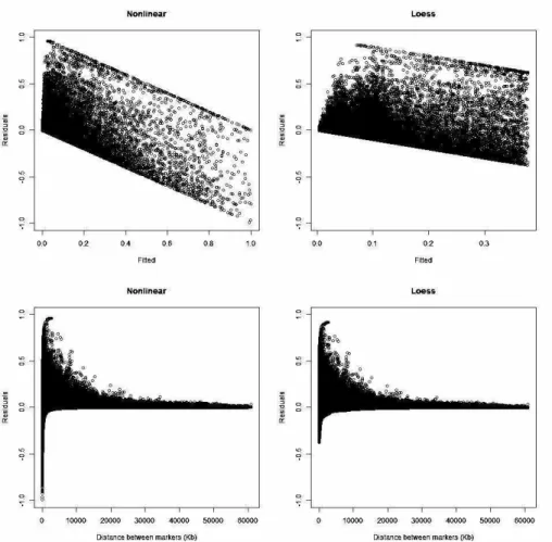
To evaluate which approach is the most appropriate to predict LD decay, we compared the fit of the nonlinear (parametric) and loess (nonparametric) regression models using the coefficient of determination (R2_{) and residual}

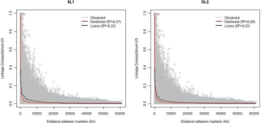
53 value was observed for loess regression (0.27 and 0.33 for nonlinear and loess regression in SL1, respectively). This indicates that a small proportion of the total variation of LD decay is explained by these models (Figure 3.1). The same pattern was observed for both lines, with the nonlinear regression model predicting higher values of LD than the loess model when distances between markers were small. Additionally, the nonlinear regression model predicted a faster decay of LD in comparison to the loess regression model.

Figure 3.1 Observed and predicted values of linkage disequilibrium (r²) in relation to the distance on SSC18 using nonlinear and loess regression for two pig lines (SL1 and DL2).

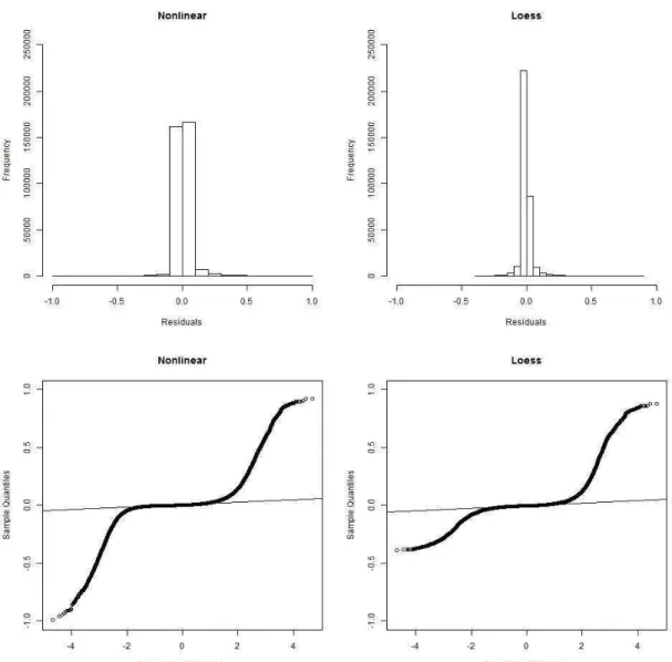
54 Figure 3.2 Residual frequency and QQ plot for nonlinear and loess regression in SL1.

55 residual values when the distance between markers was small. The DL2 residual plots were similar to Figures 3.2 and 3.3 [see Supplementary material: Figures S3.1 and S3.2].

Figure 3.3 Plots of the residuals against fitted values (top) and against the distance between markers (bottom) for nonlinear (left) and loess regression (right) in line SL1.

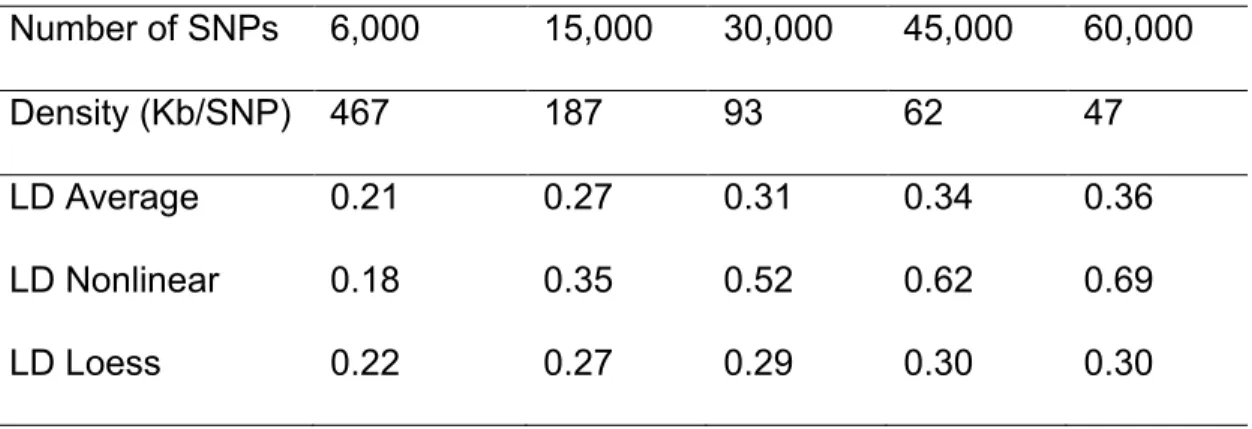
56 in the current SNP chip panel. For the smallest panel (6,000 SNPs), the average and predicted LD from both models were similar (Table 3.1). However, for higher marker densities the LD predicted using nonlinear regression was larger than both the average and the predicted LD using loess regression. The LD predicted using loess was always smaller than the empirical average, but much closer to that average value than was the prediction from the nonlinear model (Table 3.1).

Table 3.1 Predicted and average linkage disequilibrium (r²) for different marker densities.

Number of SNPs 6,000 15,000 30,000 45,000 60,000

Density (Kb/SNP) 467 187 93 62 47

LD Average 0.21 0.27 0.31 0.34 0.36

LD Nonlinear 0.18 0.35 0.52 0.62 0.69

LD Loess 0.22 0.27 0.29 0.30 0.30

57

3.3 Discussion

The comparison between nonlinear and loess regression to describe LD decay in two distinct populations showed that the loess regression model provides a better fit to the LD decay than the nonlinear model. However, when the LD decay of the two populations was compared the same result was found using a test for equality of nonlinear curves and ANOVA-type statistic for nonparametric curve comparison.

The great interest in GS and GWAS has resulted in more studies that describe (Khatkar et al., 2008; Bohmanova et al., 2010; García-Gámez et al., 2012), compare (Amaral et al., 2008; Uimari and Tapio, 2011; Badke et al., 2012; Alhaddad et al., 2013; Veroneze et al., 2013) or use LD as auxiliary information to explain the results of genetic studies (Duijvesteijn et al., 2010); however, none of these studies has evaluated how well the nonlinear and loess models fitted the data.

The real observations are widely scattered around the curves generated using the nonlinear and loess regression models for both lines. This is mainly true for short distances where the LD has large variability; in turn, this variability explains the small values of R².

58 to give shape to the curve (Schmidt et al., 2013) while at the same time requiring weaker assumptions (Andersen, 2009b).

Loess regression has been used successfully to describe nonlinear relationships between variables in genetics and animal breeding. Gulisija et al. (2007) evaluated the nonlinear patterns of inbreeding depression and found that loess improved the fit over that of first-order regression on inbreeding for milk yield traits.

The observed differences between the nonlinear and loess models may have been influenced by the design of the porcine SNP chip. When two SNPs were close together on the genome and they exhibited high LD only one of them may have been included in the SNP chip. This selection process may have lead to artificially lower averages of LD at short distances.

The equation proposed by Sved (1971) assumes that the value of LD at the intercept (when the distance between markers is zero) is equal to one; the impact of this assumption was evaluated by Corbin et al. (2010), who found that fixing the intercept at one resulted in approximate doubling of the

parameter, thereby impacting predictions of LD and effective population size. Furthermore, using modified equations that include a parameter to estimate the intercept Corbin et al. (2010) found values above two for the intercept.