Eco-geomorphology and vegetation patterns in arid and semi-arid regions

(1)

HESSD

3, 2559–2593, 2006

Eco-geomorphology and vegetation

patterns

P. M. Saco et al.

Title Page

Abstract Introduction

Conclusions References

Tables Figures

◭ ◮

Back Close

Full Screen / Esc

Printer-friendly Version

Interactive Discussion

EGU Hydrol. Earth Syst. Sci. Discuss., 3, 2559–2593, 2006

www.hydrol-earth-syst-sci-discuss.net/3/2559/2006/ © Author(s) 2006. This work is licensed

under a Creative Commons License.

Hydrology and Earth System Sciences Discussions

Papers published inHydrology and Earth System Sciences Discussionsare under open-access review for the journalHydrology and Earth System Sciences

Eco-geomorphology and vegetation

patterns in arid and semi-arid regions

P. M. Saco1, G R. Willgoose1, and G. R. Hancock2 1

School of Engineering, The University of Newcastle, Callaghan, New South Wales, 2308, Australia

2

School of Environmental and Life Sciences, The University of Newcastle, Callaghan, New South Wales, 2308, Australia

(2)

HESSD

3, 2559–2593, 2006

patterns

P. M. Saco et al.

Title Page

Tables Figures

◭ ◮

Back Close

Full Screen / Esc

EGU

Abstract

The interaction between vegetation and hydrologic processes is particularly tight in water-limited environments where a positive-feedback links water redistribution and vegetation. The vegetation of these systems is commonly patterned, that is, arranged in a two phase mosaic composed of patches with high biomass cover interspersed 5

within a low-cover or bare soil component. These patterns are strongly linked to the redistribution of runoffand resources from source areas (bare patches) to sink areas (vegetation patches) and play an important role in controlling erosion.

In this paper a new modeling framework that couples landform evolution and dynamic vegetation for water-limited ecosystems is presented. The model explicitly accounts 10

for the dynamics of runon–runo_ff areas that controls the evolution of vegetation and erosion/deposition patterns in water limited ecosystems. The analysis presented here focuses on the interaction between vegetation patterns, flow dynamics and sediment redistribution for areas with mild slopes where sheet flow occurs and banded vegetation patterns emerge. Model results successfully reproduce the dynamics of both migrating 15

and stationary banded vegetation patterns (commonly known as tiger bush). Modeling results show strong feedbacks e_ffects between vegetation patterns, runo_ffredistribution and geomorphic changes. The success at generating not only the observed patterns of vegetation but also patterns of runoff and erosion redistribution, which gives rise to modeled microtopography similar to that observed in several field sites, suggests 20

that the hydrologic and erosion mechanisms represented in the model are correctly capturing the essential processes driving these ecosystems.

1 Introduction

Arid and semi-arid areas constitute over 30% of the world’s land surface. These areas function as tightly coupled ecological-hydrological systems with strong feedbacks and 25

(3)

HESSD

3, 2559–2593, 2006

patterns

P. M. Saco et al.

Title Page

Tables Figures

◭ ◮

Back Close

Full Screen / Esc

EGU Ludwig et al., 2005). Generally, the vegetation of these regions consists of a mosaic or

pattern composed of patches with high biomass cover interspersed within a low-cover or bare soil component. A key condition for the development of these patterns is the emergence of a spatially variable infiltration field with low infiltration rates in the bare areas and high infiltration rates in the vegetated areas. This spatially variable infiltration 5

has been observed in many field studies and is responsible for the development of a runoff-runon system. Several field studies have reported much higher infiltration rates (up to 10 times) under perennial vegetation patches than in interpatch areas (Bhark and Small, 2003; Dunkerley, 2002; Ludwig et al., 2005). The enhanced infiltration rates under vegetated patches are due to improved soil aggregation and macroporosity 10

related to biological activity (e.g., termites, ants, and earthworms are very active in semi-arid areas) and vegetation roots (Tongway et al., 1989; Ludwig et al., 2005). The amount of water received and infiltrated into the vegetation patches, which includes runon from bare areas, can be up to 200% the actual precipitation (Valentin et al., 1999; Wilcox et al, 2003; Dunkerley, 2002). The runoff-runon mechanism triggers a 15

positive feedback, that is, increases soil moisture in vegetated patches reinforcing the pattern (Puigdef ´abregas et al., 1999; Valentin et al., 1999; Wilcox et al., 2003). The redistribution of water from bare patches (source areas) to vegetation patches (sink areas) is a fundamental process within drylands that may be disrupted if the vegetation patch structure is disturbed. This e_fficient redistribution of water is accompanied by 20

sediments and nutrients and allows for higher net primary productivity.

1.1 Ecohydrology of arid and semi-arid areas: processes, patterns and function

As discussed above, vegetation patterns play an important role in determining the lo-cation of runo_ffand sediment source and sink areas (Cammeraat and Imeson, 1999; Wilcox, 2003; Imeson and Prinsen, 2004). These patterns are thus functionally re-25

(4)

HESSD

3, 2559–2593, 2006

patterns

P. M. Saco et al.

Title Page

Tables Figures

◭ ◮

Back Close

Full Screen / Esc

EGU systems the spatial redistribution of flows and material is regulated by both topography

and vegetation (Tongway and Ludwig, 1997). That is, the downslope routing of water, sediments, nutrients, seeds, litter, etc, is strongly influenced by the interaction between vegetated and bare patches, which is determined by their spatial connectivity (Imeson and Prinsen, 2004). As shown by several field studies, natural vegetation patterns that 5

take decades or hundreds of years to evolve provide stabilizing properties for ecosys-tems as they are efficient in reducing overland flow and land degradation, and help ecosystems to recover from disturbance and to resist stressors (Cammeraat and Ime-son, 1999). Therefore the state of natural vegetation patterns constitutes an important indicator of ecosystem health.

10

Changes in the vegetation pattern and state in semi-arid regions are among the main indicators of the state of land degradation leading to desertification. If the vegetation cover is removed the redistribution of water is altered, inducing higher runoffrates and causing soil erosion during intense rainstorms. Disturbances, such as overgrazing, can alter the structure of vegetation patches reducing its density and/or size which leads to 15

a “leaky” system. A leaky system is less efficient at trapping runoffand sediments and loses valuable water and nutrient resources (Ludwig et al., 2004) inducing a positive-feedback loop that reinforces the degradation process (Lavee et al., 1998). When semi-arid lands become degraded, their original biotic functions are damaged and the subsequent restoration of those lands is costly and in some cases impossible.

20

1.2 Types of vegetation patterns

The most common vegetation pattern found in arid and semi-arid ecosystems is usu-ally referred to as spotted or stippled and consists of dense vegetation clusters that are irregular in shape and surrounded by bare soil (Lavee et al., 1998; Aguiar and Sala, 1999; Ludwig et al., 1999). Another common pattern is banded vegetation, also known 25

(5)

HESSD

3, 2559–2593, 2006

patterns

P. M. Saco et al.

Title Page

Tables Figures

◭ ◮

Back Close

Full Screen / Esc

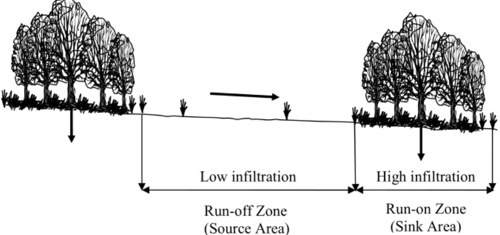
EGU and is effective in limiting hillslope erosion. The bands favor soil conservation by acting

as natural bench structures in which a gently sloping runo_ffzone leads downslope onto an interception zone (Valentin et al., 1999). Figure 1 displays a schematic diagram of a banded system showing the redistribution of water from bare patches (source areas) to vegetation patches (sink areas). Banded patterns commonly act as closed hydrologi-5

cal systems (Valentin and d’Herbes, 1999), with little net outflow and sediment coming out of the system (e.g. at the bottom of the hillslope or catchment outlet). The effect of spotted vegetation on erosion is more complex and depends on the connectivity of the bare soil areas. Wilcox et al. (2003) reported the results from the interactions between runoff, erosion, and vegetation from an experimental study in an area with 10

sparse vegetation cover (spotted vegetation) in New Mexico. They concluded that the redistribution of runoffand erosion occurs at the inter-patch scale (from bare patches to high biomass patches), with little or no effect at the hillslope scale. However, dis-turbances that modify vegetation can produce an increase in erosion rates leading to the creation of gullies and can result in irreversible degradation. That is, if vegetation 15

establishes along the new drainage gullies the overland flow pattern is lost and it is unlikely that it will re-establish itself without human intervention (Walekin-King, 1999).

Although banded patterns have been found in landscapes with a wide range of steepness, from gentle to relatively steep slopes, the key condition for their appear-ance seems to be the ability of the landscape (soil and surface conditions) to generate 20

surface runoffas sheet-flow (Valentin et al., 1999; Tongway and Ludwig, 2001). Land-scapes with incised rills and gullies, in which flow concentration precludes the gen-eration of sheet flow, do not exhibit banded vegetation. Moreover, studies in banded vegetation areas experiencing erosion and degradation have reported the disappear-ance of the banded system as soon as rills and channel incision begins (Tongway 25

(6)

HESSD

3, 2559–2593, 2006

patterns

P. M. Saco et al.

Title Page

Tables Figures

◭ ◮

Back Close

Full Screen / Esc

EGU results will be reported in a follow up paper (Saco and Willgoose, 20061).

1.3 Previous models

There is a variety of models for the simulation of coupled hydrology and vegetation dynamics in water-limited ecosystems (e.g., Aguiar and Sala, 1999; Puigdef ´abregas et al., 1999; Porporato et al., 2003; Ludwig at al., 1999; Dunkerley, 1997; Klausmeier, 5

1999; Rietkerk et al., 2002; Gilad et al., 2004 ; Boer and Puigdef ´abregas, 2005). How-ever, not all of them include the interactions between water re-distribution and dynamic vegetation patterns. Recent models that capture the interaction between spatial wa-ter redistribution and vegetation patwa-terns can be divided in two main groups. The first group includes models developed to simulate water redistribution for a fixed spa-10

tial vegetation pattern (Puigdef ´abregas et al., 1999; Ludwig at al., 1999; Boer and Puigdef ´abregas, 2005). These type of models are used to understand the effect of vegetation patterns on erosion and/or water redistribution at short time scales (e.g., from storm event to annual timescales), but do not include feedback effects that occur at longer time scales. The evolution of vegetation patterns occurs at time scales vary-15

ing from several years to several decades and thus these models can not be directly used to asses the impact of climate change or grazing pressure. The second group of models simulates the development and evolution of vegetation patterns as a function of water redistribution (Dunkerley, 1997; Klausmeier, 1999; HilleRisLambers et al., 2001; Rietkerk et al., 2002; Gilad et al., 2004). These models have provided valuable insight 20

into the mechanisms responsible for the emergence and self-organization of the ob-served vegetation patterns in arid and semi-arid areas. However, they do not include the dynamic effect of erosion-deposition processes and their feedback effects on flow routing, soil moisture and vegetation pattern dynamics. That is, erosion-deposition mechanisms change topography affecting surface water redistribution and soil mois-25

1

(7)

HESSD

3, 2559–2593, 2006

patterns

P. M. Saco et al.

Title Page

Tables Figures

◭ ◮

Back Close

Full Screen / Esc

EGU ture patterns, which in turn affect the evolution of the vegetation pattern at longer time

scales. These non-linear self-reinforcing e_ffects may lead in some cases to the de-sertification of the system (Lavee et al., 1998). This type of feedback effects can be studied using a coupled dynamic vegetation – landform evolution model that incorpo-rates evolving patterns of vegetation as the one described in this paper.

5

Recent research has incorporated the effect of dynamic vegetation on erosion and landform evolution for humid areas in which soil moisture does not limit vegetation growth (Collins et al., 2004; Istanbulluoglu and Bras, 2005). The results provide impor-tant insight into the effects of vegetation dynamics on geomorphic processes for humid areas. Unlike these previous studies the results presented here are for water limited 10

environments, and therefore plant growth depends on soil moisture availability which is assumed to be the most important limiting resource (i.e., plant growth is assumed not to be limited by nutrient availability).

In the following sections we investigate the interactions between dynamic vegetation patterns and geomorphology in banded vegetation systems. This analysis uses a new 15

coupled dynamic vegetation – landform evolution model. In Sect. 2 we describe the dynamic vegetation model. Section 3 provides a brief description of the SIBERIA land-form evolution model (Willgoose et al., 1991) used in this study. Section 4 explains how the models are coupled and the flow of information between the coupled mod-els. Section 5 describes the simulation results for banded vegetation systems and final 20

conclusions are summarized in Sect. 6.

2 Dynamic vegetation model

In this section we describe a new model for the development of vegetation patterns in water limited ecosystems. The dynamic vegetation model describes the dynamics of three state variables: plant biomass density (P; mass/area), soil moisture (M; vol-25

(8)

Un-HESSD

3, 2559–2593, 2006

patterns

P. M. Saco et al.

Title Page

Tables Figures

◭ ◮

Back Close

Full Screen / Esc

EGU like these previous models, our model incorporates a model for surface water routing.

The e_ffect of seed dispersal by overland flow is also incorporated as a possible mech-anism for the emergence of stationary vegetation bands not simulated by previous models.

2.1 Overland flow dynamics 5

The partial di_fferential equations governing the redistribution of overland flow (run-on and run-off) are the conservation of mass and momentum. The full dynamic form of these equations for the description of free surface flow is known as the Saint Venant equations. A simplified version of the Saint Venant equations is the kinematic wave ap-proximation, which includes a simplified momentum equation applicable to most prac-10

tical hydrologic conditions where backwater effects are considered negligible (Vieux, 1991). The conservation of water mass (continuity) can be written as:

∂h(x, y, t)

∂t =−∇ ·q(x, y, t)+R(x, y, t)−I(x, y, t) (1)

whereh [m] is the flow depth, q [mm m/day] is the flow discharge per unit width, R

[mm/day] is the rainfall rate,I [mm/day] is the infiltration rate, x and y [m] denote the 15

position coordinates,t [day] is time, ∇·is the divergence operator, and the bold italic letters indicate vector quantities.

The conservation of momentum using the kinematic wave assumption is described as (Henderson and Wooding, 1964; Woolhiser and Liggett, 1967; Vieux, 1991; Mitas and Mitasova, 1998):

20

S_o=S_f (2)

in which the friction slope (Sf) is assumed to be the same as the land surface slope

(So). That is, kinematic wave theory assumes that shallow water waves are long and

(9)

HESSD

3, 2559–2593, 2006

patterns

P. M. Saco et al.

Title Page

Tables Figures

◭ ◮

Back Close

Full Screen / Esc

EGU Mitasova, 1998), so that the overland flow discharge per unit width can be expressed

as:

q(x, y, t)= c_nnh(x, y, t)53S

o(x, y, t)

1

2 (3)

wheren is Manning’s roughness coefficient and C_n the constant for unit conversion (m mm−32 _day−1_{). We use a spatially constant} n _{for simplicity, but changes in} n _due 5

to changes in local biomass can be included in the model (Istanbulluoglu and Bras, 2005).

A quasi steady approximation is adopted here and Eq. (1) is solved for steady state conditions (∂h/∂t=0). This is justified since the time scale at which the rate of change of runoffredistribution occurs (seconds to hours) is much faster than that at which plant 10

biomass occurs (days for grasses to months for shrubs). Therefore, a time step of 0.5 day is used to model vegetation change and the amounts ofqand hare represented

by their equilibrium values which occur at much smaller time scales. The steady state approximation is also considered to provide an adequate estimate of overland flow for land management applications (Flanagan and Nearing, 1995; Mitas and Mitasova, 15

1998).

The magnitude and direction of overland flow and the slope (S_o) can change with time in response to erosion-deposition processes. The direction of the flow vectorq

and the surface slopeSoare computed in the steepest descent direction and estimated

(and updated) by the landform evolution model (more details are given in Sect. 4). For 20

the cases analyzed in this paper, the flow is one-dimensional, that is the direction of the flow lines (or stream tubes as defined by Vieux, 1991) coincide with the x-axis and corresponds to the steepest descent direction without invoking any approximation. The spatial and temporal coordinates (x, y, t) are not included in any of the equations that follow to simplify the notation.

25

(10)

HESSD

3, 2559–2593, 2006

patterns

P. M. Saco et al.

Title Page

Tables Figures

◭ ◮

Back Close

Full Screen / Esc

EGU al., 1997, 1998). Investigations of this type confirm that infiltration rate is not solely

de-termined by the soil matrix, but rather depends on a range of other factors including the dynamics of the flow crossing the surface and the extent to which the form and ampli-tude of the microtopography allows or precludes broad sheet flow or more concentrated thread flow. Dunne et al. (1991) reported di_fferences in soil macroporosity and conse-5

quently in water uptake (infiltration) rates between low-lying and elevated parts of the microtopography. Greater local infiltration rates in elevated locations contribute to an observed increase in infiltration rate with rainfall intensity, and to an apparent increase of infiltration rates with hillslope length, that arises as flow depth increases downslope and more completely inundates the microtopography. Experiments on crusted surfaces 10

(Fox et al., 1998) suggest that spatial variability in seal characteristics, which vary with microtopography, can strongly influence the response of infiltration under conditions of varying ponding depth. That is, an increase in ponding depth inundates areas of higher hydraulic conductivity and infiltration rate increases significantly. The observa-tions by Dunkerley (2002) on the spatial patterns of soil moisture and infiltration rate in 15

a banded mulga woodland in arid central Australia provide additional evidence of the dependence of infiltration on flow depth for arid regions. He found that infiltration rates are highest close to tree stems (usually located in higher areas of the microtopogra-phy within vegetation patches or groves) and decline rapidly with increasing distance. Therefore, as the vegetated areas within the groves become inundated with increasing 20

flow depth, the apparent infiltration rate of the groves will increase.

We assume that infiltration,I, depends on the biomass densityP (Walker et al., 1981) and the overland flow depthhaccording to (HilleRisLambers et al., 2001; Rietkerk et al., 2002):

I=αhP +k2Wo P +k2

(4) 25

whereα(day−1) defines the maximum infiltration rate,k2(g m −2

(11)

HESSD

3, 2559–2593, 2006

patterns

P. M. Saco et al.

Title Page

Tables Figures

◭ ◮

Back Close

Full Screen / Esc

EGU the dependence of the infiltration rateI on biomass density P (for W_o=1 there is no

biomass dependence, forWo<<1 the infiltration rate increases strongly with increased

biomass density, and forW_o>1 infiltration rate decreases with biomass density, which though mathematically possible, is physically unrealistic). For any given value of flow depth h, the infiltration is lowest for bare soil conditions (αhWo) and increases with

5

increasing biomass density to asymptotically approach the maximum value (αh).

2.2 Soil moisture dynamics

The soil moistureM(mm) is defined as the plant available soil water (that is, the total soil moisture isMt=M +Mmin, whereMmin is the wilting point). Soil moisture changes are modeled using a simple single bucket approach, in which gains are due to infiltration 10

and losses are due to plant water uptake, evaporation and deep drainage:

∂M

∂t =I−gmax M M+k1

P−r_wM (5)

The second term represents soil water uptake by plants, which is assumed to be a saturating function of soil moisture availability (HilleRisLambers et al., 2001; Rietkerk et al., 2002). gmax[mm g

−1

m−2day−1] is the maximum specific water uptake (asymp-15

totic value of water uptake per unit of biomass density asM increases) andk1(mm) is the half-saturation constant of specific water uptake. WhenM=k1,water uptake (and

growth rate, see Eq. 6) is at half its maximum rate. Therefore, the half-saturation con-stant describes the water uptake characteristics of different plant species, with lowk1 values indicating the ability of plants to thrive under water stress (low soil moisture) con-20

(12)

HESSD

3, 2559–2593, 2006

patterns

P. M. Saco et al.

Title Page

Tables Figures

◭ ◮

Back Close

Full Screen / Esc

EGU 2.3 Vegetation dynamics

The rate of change of plant biomass densityP (g m−2) is determined by plant growth, senescence, and spatial dissemination of vegetation due to seed or vegetative propa-gation, and can be expressed as:

∂P

∂t =cgmax M M+k1

P −d P +Dp∇2P − ∇ ·qsd (6)

5

The first term represents plant growth, which is assumed to be directly proportional to water uptake (transpiration) with c (g mm−1m−2) being the conversion parameter from water uptake to plant growth. Water uptake by roots is assumed to equal actual transpiration, without considering any variations in the water storage of vegetation. The main control of plant production is assumed to be water limitation, so that when 10

water supply through rain or runon is insufficient plant transpiration becomes less than potential (the maximum asymptotic plant growth is given bycgmax when soil moisture is not limiting), linearly decreasing plant growth. Nutrient availability is assumed not to limit plant growth at this production level. The second term represents biomass density loss and d (day−1) is the specific loss coefficient of biomass density due to 15

mortality (disturbances such as vegetation removal by grazing can be included in this term through a higherd).

The last two terms account for plant dispersal. Dp(m2day

−1

) in the third term is the dispersal coefficient for isotropic processes such as wind and animal action (termites are important agents for seed dispersal in many arid and semi-arid areas) and∇2 is 20

the Laplacian operator. The fourth term accounts for plant propagation caused by the transport of seed biomass by overland flow. The seed biomass transport vector, q_sd

(gm−1day−1), has a magnitude,q_sd given by:

q_sd =c1qP forc1q < c2

qsd =c2P forc1q > c2

(13)

HESSD

3, 2559–2593, 2006

patterns

P. M. Saco et al.

Title Page

Tables Figures

◭ ◮

Back Close

Full Screen / Esc

EGU and the direction of the overland flow (in this case, steepest descent direction). c1

(mm−1andc2(m day −1

) are process parameters. The transport of seed biomass in the flow direction depends on the magnitude and direction of overland flow discharge (i.e., transport limited conditions for seed redistribution by overland flow), but its maximum value (c2P) depends on the total amount of seed biomass available for overland flow 5

dispersal (i.e., production limited conditions) which is assumed to be proportional to the total biomass densityP.

Previous models (HilleRisLambers et al., 2001; Rietkerk et al., 2002; Gilad et al., 2004) incorporated plant dispersal, through seed or vegetative propagation by includ-ing a diffusion term (the third term in Eq. 6) but they did not account for the transport of 10

seeds by overland flow (fourth term). However, the redistribution of seeds by overland flow has been identified in field experiments as one possible explanation for the ob-served stationarity of vegetation bands (Dunkerley, 2002). As explained in more detail in Sect. 5.2, this model reproduces both stationary bands (as observed in Australia) and traveling vegetation bands (observed in Sudan and some other locations).

15

3 Landform evolution model

SIBERIA is a physically based model of the evolution of landforms under the action of fluvial erosion, creep and mass movement. The elevations within the catchment are simulated by a mass-transport continuity equation applied over geologic time scales. Mass-transport processes considered include fluvial sediment transport, such as those 20

(14)

HESSD

3, 2559–2593, 2006

patterns

P. M. Saco et al.

Title Page

Tables Figures

◭ ◮

Back Close

Full Screen / Esc

EGU landform at a point follows directly from the mass conservation of sediment:

∂z

∂t =U −

∇ ·q_s

ρ_s(1−n_p) +∇ ·qd

!

(8)

whereU (m/day) is the rate of tectonic uplift, ∇· is the divergence operator,q_s is the

fluvial sediment transport per unit width (T/day/m width),q_d is the diffusive mass

trans-port per unit width (m3/day/m width),ρ_sis the density of the sediment,n_pis the porosity 5

of the sediment and the bold italic indicates vector quantities. Generically, Eq. (8) does not assume any particular sediment transport processes since it is simply a statement of sediment transport continuity. Rather it is our adopted process representation forq_s

andq_d that determines the processes modeled.

Sediment transport by overland flow is modeled as (transport limited conditions): 10

qs=β1qm1Sn1 (9)

whereq is the surface runoff per unit width (estimated in the vegetation model, see Sect. 2.1),S is the slope in the steepest downslope direction,m1 and n1 are param-eters in the fluvial transport model, andβ1 is the rate of sediment transport, function of sediment grain size and vegetation cover, analogous to theKfactor in other erosion 15

models, e.g. CREAMS, USLE. Note that a transport limited model is needed in order to capture the effect of surface water redistribution on erosion/deposition processes. That is, the existence of spatially heterogeneous vegetation and spatially varying infiltration rates induces the appearance of areas of surface runoffthat trigger erosion and areas of run-on that induce sediment deposition.

20

Biomass cover is one of the key factors influencing soil erodibility. This is due to the positive effect of the vegetation on improving soil quality through organic matter and litter contribution. Also, a more active fauna and flora, which is generated due to com-bined effect of enhanced weathering, enhanced infiltration and a less contrasted micro-climate, produces stronger aggregates (Zhang, 1994; Cerd `a, 1998). Under semiarid 25

(15)

HESSD

3, 2559–2593, 2006

patterns

P. M. Saco et al.

Title Page

Tables Figures

◭ ◮

Back Close

Full Screen / Esc

EGU which is strongly influenced by vegetation. Field studies in semiarid areas show that the

minimum soil aggregation is found in bare areas and increases with vegetation cover (Cerd `a, 1998). Accordingly, we model the decrease in soil erodibility with increasing biomass density through the parameter β1 that is assumed to linearly decrease as biomass density increases as (similar to other linear formulations in the literature, e.g., 5

Boer and Puigdef ´abregas, 2005):

β1=βb(1−βvP) for βvP <1−

βmin

βb

β1=βmin for βvP ≥1−

β_min

βb

(10)

That is, the erodibility parameter is maximum for bare soil (βb) and is assumed to

decrease linearly with increasing biomass density at a rate given byβ_v to a minimum value given byβmin.

10

Diffusive transport processes (e.g. rainsplash, soil creep) are modeled as:

qd =DS (11)

whereD (m3/day/m width) is the diffusion coefficient, assumed here to be spatially constant. This diffusion model is widely used to conceptualize mass movement (Ah-nert, 1976). Other forms of mass wasting like landslides and debris flows were not 15

included in the analysis since they are not important in the mild-slope areas that are the main focus of this study. The direction of the vectorq_d is again assumed to be in

the steepest downslope direction which is consistent with the assumption for overland flow estimated using Eq. (3) and involves no approximation for the cases presented in this paper.

20

4 Coupled model

(16)

HESSD

3, 2559–2593, 2006

patterns

P. M. Saco et al.

Title Page

Tables Figures

◭ ◮

Back Close

Full Screen / Esc

EGU (biomass density), and geomorphic (elevations and slopes) variables. The vegetation

model and landform evolution model (SIBERIA) share the same computational grid but the processes simulated in each model operate over different time scales, and are therefore executed at different time steps. The time step in SIBERIA is based on the duration of erosive time scales (days to years), whereas the vegetation model that 5

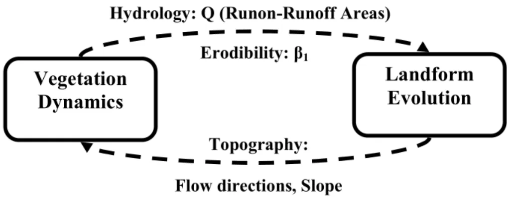
includes the computation of surface flow redistribution, soil moisture and vegetation dynamics utilizes shorter time steps (sub-daily). The models have not been tightly cou-pled to improve computational speed and performance. Figure 2 shows the flow of information between both models. The vegetation model computes the evolution and spatial distribution of biomass density and overland flow. These variables are input into 10

the landform evolution model that computes sediment transport. Biomass information is used to update the erodibility parameters which, together with overland flow distribu-tion, are used to compute spatially distributed erosion and deposition volumes and to update elevations. The new topographic surface is then used to compute updated flow directions and slopes that are input to the next step of the vegetation model.

15

5 Results and discussion

The simulations analyzed in this section correspond to a two-dimensional hillslope with an area of 200 m×200 m and a grid spacing of 2 m. No flow boundary conditions were set for the upstream and lateral borders, while free flow boundary conditions were used in the downstream boundary (drainage was allowed through the complete downhill 20

border of the domain). The initial hillslope profile corresponds to a planar slope of 1.4% that is typical of areas with banded vegetation in Australia (Dunkerley and Brown, 1999). The initial vegetation consisted of biomass peaks randomly distributed in 1% of the grid elements. The rest of the grid elements were set to bare soil conditions. The precipitation for the simulations shown in this paper was set to 320 mm/year (high 25

(17)

HESSD

3, 2559–2593, 2006

patterns

P. M. Saco et al.

Title Page

Tables Figures

◭ ◮

Back Close

Full Screen / Esc

EGU The parameters for vegetation dynamics used in this analysis (shown in Table 1)

were adopted following those reported by Rietkerk et al. (2002) for the analysis of veg-etation patterns using a similar model. The surface roughness coefficient (i.e., Man-ning’s coefficient) corresponds to commonly accepted values in vegetated surfaces. These parameters give rise to low biomass vegetation that evolves into equilibrium 5

conditions rapidly. Different sets of parameters can be selected to simulate growth and development of vegetation dynamics similar to that of shrubs and grasses for semi-arid areas reported in previous studies (Sparrow et al., 1997; Gao and Reynolds, 2003). Table 2 shows the parameters for the erosion processes included in the landform evo-lution model used in all simulations, chosen from the range of recommended values 10

(Willgoose, 2004). As seen in Table 2, the simulations presented in this paper corre-spond to the simpler case of declining equilibrium conditions (U=0).

5.1 Self organization into banded vegetation patterns

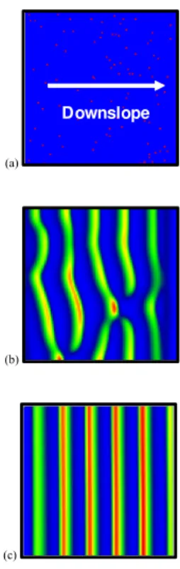
The initial distribution of biomass density is shown in Fig. 3a. On a hillslope in which overland flow occurs predominantly in only one direction (as sheet flow with no flow 15

concentration) the coupled model generates regular vegetation bands perpendicular to the flow direction (tiger bush or banded type of pattern). For the parameters shown in Tables 1 and 2, stationary vegetation bands have completely developed for t>15 years. Figures 3b and c shows two stages in band development for t=560 days and t=15 years respectively.

20

The evolution of vegetation bands follows from the functioning of the system as a series of runoff-runon areas that arise in response to the mechanisms of facilitation of infiltration and competition for soil moisture by plants. Runoff is produced in the bare areas and increases downslope towards the upper boundary of the vegetated patches (groves). Vegetation colonizes (by growth and dispersion) areas with sufficient 25

(18)

HESSD

3, 2559–2593, 2006

patterns

P. M. Saco et al.

Title Page

Tables Figures

◭ ◮

Back Close

Full Screen / Esc

EGU passed on to the vegetated areas situated further downslope. After a distance set by

runon availability, soil moisture becomes inadequate for plant growth requirements, and biomass decreases (the grove dies out) giving way to an area with very low biomass density (intergrove). The intergrove has low infiltration rates allowing for a progressive increase in runo_ffvolume downslope from the grove boundary. When su_fficient runo_ff 5

becomes available to satisfy soil moisture requirements, another patch of vegetation emerges (grove).

The bands grow laterally (through seed dispersal) because there is no competition for water with other lateral plants. That is, plants located at the same distance from the upstream vegetation boundary receive the same amount of water, therefore there is no 10

lateral competition for water and the bands expand laterally allowing for the formation of parallel bands typical of banded systems. Note that this is the case because there is no flow concentration, surface flow is in the form of sheet flow and flowlines are parallel (perpendicular to the groves).

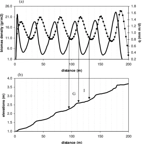
Figure 4a, shows the distribution of biomass along the longitudinal profile. The 15

biomass cover is continuous, but its spatial distribution displays high densities (groves) and low densities (intergroves) in a periodic pattern. Figure 4b shows the overland flow for the stationary vegetation bands, showing that the spatial variability of runoff and that of biomass density are out of phase. That is, runoffis higher in the areas with the minimum biomass density (low infiltration) and lower in the areas with higher biomass 20

(high infiltration).

5.2 Stationary and migrating bands

As mentioned in Sect. 2, the appearance of stationary bands is due to the effect of anisotropic seed dispersal resulting from the preferential redistribution of seeds by surface flow downslope. This term was not included in previous models which only 25

(19)

HESSD

3, 2559–2593, 2006

patterns

P. M. Saco et al.

Title Page

Tables Figures

◭ ◮

Back Close

Full Screen / Esc

EGU support both the existence of migrating bands and stationary bands in different

land-scapes (Valentin et al., 1999; Ludwig and Tongway, 2001). As discussed by Valentin et al. (1999), evidence of upslope migration remains scarce and the direct observa-tions of band movement over short time spans do not give compelling information due to the slow velocity of the migrating bands. In particular, several field studies in Aus-5

tralia have reported the existence of stationary bands and one of the possible reported mechanisms that might prevent the bands from traveling upstream is seed redistribu-tion by overland flow. Observaredistribu-tions by Dunkerley and Brown (2002) for a 6-year period on a banded chenopod shrubland in Western New South Wales in Australia show no evidence of systematic migration of grove–intergrove boundaries. They found that the 10

majority of the bands remained in place within the limits of measurement accuracy (typically, 0.5 m). Similarly, Dunkerley (2002) found no evidence of systematic upslope pattern migration over a 24-year study period on a banded pattern of Mulga trees near Alice Springs in Australia. Accordingly, Dunkerley and Brown (2002) and Dunkerley (2002) concluded that these results provided field evidence in contradiction with ex-15

isting numerical models based on ‘runoff–runon’ mechanisms for pattern generation that predict upslope migration of patterns (for example, Klausmeier, 1999; Rietkerk et al., 2002; among others). However, as shown here, our model based on runoff-runon mechanisms reproduces both stationary and migrating bands.

Migrating bands were reproduced by imposing c2=0 with all other parameters re-20

maining the same as shown in Table 1. For the case of migrating bands, the “dynamic” patterns reproduced in our simulations are slightly different from those reported previ-ously (e.g., in Rietkerk et al., 2002). This is mainly due to the difference in boundary conditions used in our analysis. As we are interested in the interactions between vege-tation patterns, flow redistribution and erosion-deposition in hillslopes and its impact on 25

(20)

HESSD

3, 2559–2593, 2006

patterns

P. M. Saco et al.

Title Page

Tables Figures

◭ ◮

Back Close

Full Screen / Esc

EGU 5.3 Geomorphology-ecohydrology interactions

Figure 4b shows the simulated hillslope profile (elevations) for t=500 years. As seen in this Figure, the initially planar hillslope evolves into a profile with stepped microto-pography. This type of hillslope profile is in agreement with the field data obtained by Dunkerley and Brown (1995, 1999) in both banded mixed shrubland-grassland and 5

chenopod shrubland communities in Australia. Figure 5 shows the hillslope topogra-phy for one of their study sites. As observed in this Figure the hillslope surface profile is composed of a series of concave-upward elements (Dunkerley and Brown, 1999). Figure 6a shows a schematic representation of the stepped microtopography gener-ated by the model. Figure 6b shows the schematic representation of the stepped 10

microtopography reported by Dunkerley and Brown (1999). These Figures show good agreement; the series of microtopographic elements represented in both Figures have similar shape and have the runon zone located upslope and the runoff zone below. What is particularly interesting about the simulated hillslope profile shown in Fig. 4 and represented in Fig. 6a is that most of the vegetated bands (groves) are located in the 15

regions of higher slope, and not on the flatter areas as could have been expected from differences in erodibility between bare and vegetated areas.

The concave-upward element in Figs. 6a and b, composed of an upper grove and the lower intergrove, exhibits a smooth decline in gradient and displays no break of slope. Figure 6b also includes a slight depositional ridge which is not reproduced in 20

our model (Fig. 6a) but that was only observed in some of the field sites studied by Dunkerley and Brown (e.g., there are no evident depositional ridges in the transect shown in Fig. 5). Each concave-upward element functions as a source-sink unit. In the intergrove areas increasing amounts of sediments (and nutrients) are removed by runo_ffthat increases with distance from the upper grove boundary. At the boundary 25

(21)

HESSD

3, 2559–2593, 2006

patterns

P. M. Saco et al.

Title Page

Tables Figures

◭ ◮

Back Close

Full Screen / Esc

EGU is in agreement with observations reporting that both ponding of water and sediment

deposition are highest in the upslope margin of the groves (Dunkerley and Brown, 1999). The simulated runon decreases downslope from the grove upper boundary, therefore the amount of sediments deposited also decreases. The simulated erosion-depositional functioning of the pattern successfully reproduces observations.

5

Elsewhere in Australia, similar microtopography has been observed in banded veg-etation areas. Topographic profiles of patterned Mulga in central Australia (Berg and Dunkerley, 2004) display stepped microtopography with intergroves located on lower gradients concave-upward areas and groves found on steeper gradients and straighter (not concave-upward) areas. This same type of microtopography has been observed 10

in another site of patterned Mulga in central Australia (Slatyer, 1961) and in Western Australia (Mabbutt and Fanning, 1987). However the stepped microtopography of pat-terned Mulga lands in eastern Australia (south-western Queensland and northwestern New South Wales) is di_fferent. Mulga groves occur on nearly level “steps” in the land-scape and there is a gradual drop into the grove and a more distinct “scarp” below the 15

grove (Tongway and Ludwig, 1990).

It has been proposed by several researchers that the appearance of the stepped microtopography may be linked to differences in soil erosion rates across the patterned landscape (Tongway and Ludwig, 1990; Dunkerley, 2002) and redistribution (deposi-tion) of soil in runon (sink) areas. The modeling results presented here are the first that 20

have been published that capture this dynamics and reproduce the observed stepped microtopography. A more complete sensitivity analysis of the erosion and runoff re-distribution parameters is still needed to see if the differences in microtopography ob-served in different landscapes (described in the previous paragraph) can be explained by differences in process parameters.

25

(22)

HESSD

3, 2559–2593, 2006

patterns

P. M. Saco et al.

Title Page

Tables Figures

◭ ◮

Back Close

Full Screen / Esc

EGU not evolve into steeped microtopography.

6 Summary and conclusions

A coupled dynamic vegetation – landform evolution model for water limited ecosys-tems has been developed. This model was used to explore the interactions between patterned vegetation and erosion by explicitly accounting for the e_ffect of dynamic water 5

redistribution not considered in previous models (Ludwig et al., 1999; Puigdef ´abregas et al., 1999). That is, previous models did not account for the dynamic effect of erosion-deposition processes and their feedback e_ffects on flow routing, soil moisture and veg-etation pattern dynamics. The erosion-deposition mechanisms change topography af-fecting surface water redistribution and soil moisture patterns.

10

The analysis presented in this paper is focussed on the interaction between vege-tation patterns, flow dynamics and sediment redistribution for areas with mild slopes where sheet flow occurs and banded vegetation patterns emerge. The extent of the appearance of this type of patterns is very important worldwide (see Fig. 3 in Valentin et al., 1999, for a map showing the global distribution of banded patterns) and the 15

results from our model explaining the evolution and dynamic interactions between veg-etation, hydrology and geomorphic changes have enough relevance to present them in isolation from the results for other type of patterns. When flow concentration occurs the model generates different vegetation patterns (spots and stripes aligned to the direc-tion of flow) and the redistribudirec-tion of flow and sediments is remarkably different from the 20

results reported here for banded vegetation. These results will be reported elsewhere (Saco et al., 20061).

On a hillslope in which overland flow occurs predominantly in only one direction (as sheet flow with no flow concentration) the coupled model reproduces:

– Vegetation bands perpendicular to the flow direction (tiger bush or banded type of 25

(23)

HESSD

3, 2559–2593, 2006

patterns

P. M. Saco et al.

Title Page

Tables Figures

◭ ◮

Back Close

Full Screen / Esc

EGU

– Both stationary bands as observed in Australia and migrating bands as observed in other regions (not shown).

– Hillslope profiles with stepped microtopography as that observed in several field sites with stationary banded vegetation in Australia (Dunkerley and Brown 1995, 1999). These modelling results are the first that have been published that capture 5

this dynamics and reproduce the observed stepped microtopography.

– Planar topography for the case of migrating bands. That is, in this case there is no development of stepped microtopography.

The success at generating not only the observed patterns of vegetation, but also pat-terns of runoffand erosion redistribution (which originates the observed microtopogra-10

phy) suggests that the hydrologic and erosion mechanisms represented in the model are correctly capturing the essential processes driving these ecosystems. Understand-ing the non-linear interactions between vegetation patterns, runoffprocesses and ero-sion in arid and semi-arid areas becomes of crucial importance due to current accel-erated changes in land use and climate. The model can be used to study feedback 15

effects between geomorphology and vegetation under land use or climate change.

References

Ahnert, F.: The role of the equilibrium concept in the interpretation of landforms of fluvial erosion and deposition, in: L’evolution des versants, edited by: Macar, P., 23–41, University of Liege, Liege, 1967.

20

Aguiar, M. R. and Sala, O. E.: Patch structure, dynamics and implications for the functioning of arid ecosystems, Trends in Ecology and Evolution, 14, 273–277, 1999.

Berg, S. S. and Dunkerley, D. L.: Patterned Mulga near Alice Springs, central Australia, and the potential threat of firewood collection on this vegetation community, J. Arid Environ., 59, 313–350, 2004.

(24)

HESSD

3, 2559–2593, 2006

patterns

P. M. Saco et al.

Title Page

Tables Figures

◭ ◮

Back Close

Full Screen / Esc

EGU Bhark, E. W. and Small, E. E.: Association between plant canopies and the spatial patterns of

infiltration in shrubland and grassland of the Chihuahuan Desert, New Mexico, Ecosystems, 6, 185–196, 2003.

Boer, M. and Puigdef ´abregas, J.: Effects of spatially structured vegetation patterns on hillslope erosion in a semiarid Mediterranean environment: a simulation study, Effects of vegetation 5

patterns on erosion, Earth Surface Processes and Landforms, 30, 149–167, 2005.

Cammeraat, L. H and Imeson, A. C.: The evolution and significance of soil-vegetation patterns following land abandonment and fire in Spain, Catena, 37(1–2), 107–127, 1999.

Cerd `a, A.: Soil aggregate stability under different Mediterranean vegetation types, Catena, 32, 73–86, 1998.

10

Collins, D. B. G., Bras, R. L., and Tucker, G. E.: Modeling the effects of vegetation-erosion cou-pling on landscape evolution, J. Geophys. Res., 109, F03004, doi:10.1029/2003JF000028, 2004.

d’Herbes, J. M, Valentin, C., Tongway, D., and Leprun, J. C.: Banded Vegetation Patterns and related Structures, in Banded vegetation patterning in arid and semiarid environments: 15

ecological processes and consequences for management, Ecological studies 149, Springer-Verlag, New York, USA, 1–19, 2001.

Dunkerley, D. L.: Banded vegetation: development under uniform rainfall from a simple cellular automation model, Plant. Ecol., 129, 103–111, 1997.

Dunkerley, D. L.: Infiltration rates and soil moisture in a groved Mulga community near Alice 20

Springs, arid central Australia: evidence for complex internal rainwater redistribution in a runoff-runon landscape, J. Arid Environ., 51, 199–219, 2002.

Dunkerley, D. L. and Brown, K. J.: Runoffand runon areas in a patterned chenopod shrubland, arid western New South Wales, Australia: characteristics and origin, J. Arid Environ., 30, 41–55, 1995.

25

Dunkerley, D. L. and Brown, K. J.: Banded vegetation near Broken Hill, Australia: significance of surface roughness and soil physical properties, Catena, 37, 75–88, 1999.

Dunkerley, D. L. and Brown, K. J.: Oblique vegetation banding in the Australian arid zone: implications for theories of pattern evolution and maintenance, J. Arid Environ., 51, 163– 181, 2002.

30

Dunne, T., Zhang, W., and Aubry, B. F.: Effects of rainfall, vegetation, and microtopography on infiltration and runoff, Water Resour. Res., 9, 2271–2285, 1991.

(25)

HESSD

3, 2559–2593, 2006

patterns

P. M. Saco et al.

Title Page

Tables Figures

◭ ◮

Back Close

Full Screen / Esc

EGU Flanagan, D. C. and Nearing M. A. (Eds.): WEPP: USDA-Water Erosion Prediction Project,

NSERL Rep. 10, National Soil Erosion Lab., U.S. Dep. of Agric., Laffayette, Indiana, 1995. Fox, D. M., Bryan, R. B., and Price, A. G.: The influence of slope angle on infiltration rate and

surface seal characteristics for interrill conditions, Geoderma, 80, 181–194, 1997.

Fox, D. M., Le Bissonnais, Y., Bruand, A.: The effect of ponding depth on infiltration in a crusted 5

surface depression, Catena, 32(2), 87–100, 1998.

Gao, Q. and Reynolds, J. F.: Historical shrub-grass transitions in the northern Chihuahuan Desert: modeling the effects of shifting rainfall seasonality and event size over a landscape gradient, Global Change Biol., 9, 1–19, 2003.

Gilad, E., von Hardenberg, J., Provenzale, A., Schachak, M., and Meron, E.: Ecosystem 10

Engineers: From Pattern Formation to Habitat Creation, Phys. Rev. Lett., 93(9), 098105, doi:10.1103/PhysRevLett.93.098105, 2004.

Henderson, F. M. and Wooding, R. A.: Overland flow and groundwater flow from a steady rainfall of finite duration, J. Geophys. Res., 69, 1531–1540, 1964.

HilleRisLambers, R., Rietkerk, M., van den Bosch, F., Prins, H. H. T., and de Kroon, H.: Vege-15

tation pattern formation in semi-arid grazing systems, Ecology, 82, 50–61, 2001.

Imeson, A. C. and Prinsen, H. A. M.: Vegetation patterns as biological indicators for identifying runoffand sediment source and sink areas for semi-arid landscapes in Spain, Agriculture, Ecosyst. Environ., 104, 333–342, 2004.

Istanbulluoglu E. and Bras, R. L.: Vegetation-modulated landscape evolution: Effects of veg-20

etation on landscape processes, drainage density, and topography, J. Geophys. Res., 110, F02012, doi:10.1029/2004JF000249, 2005.

Julien, P. Y., Saghafian, B., and Ogden, F. L.: Raster-based hydrologic modeling of spatially varied surface runoff, Water Resour. Bull., 3(3), 523–536, 1995.

Klausmeier, C. A.: Regular and irregular patterns in semiarid vegetation, Science, 284, 1826– 25

1828, 1999.

Lavee, H., Imeson, A. C., and Sarah, P.: The impact of climate change on geomorphology and desertification along a Mediterranean–arid transect, Land Degrad. Dev., 9, 407–422, 1998. Ludwig, J. A., Wilcox, B. P., Breshears, D. D., Tongway, D. J., and Imeson, A. C.: Vegetation

patches and runoff-erosion as interacting ecohydrological processes in semiarid landscapes, 30

Ecology, 86(2), 288–297, 2005.

(26)

HESSD

3, 2559–2593, 2006

patterns

P. M. Saco et al.

Title Page

Tables Figures

◭ ◮

Back Close

Full Screen / Esc

EGU semi-arid woodlands, Australia, Catena, 37, 257–273, 1999.

Ludwig, J. A., Tongway, D. J., Bastin, G., and James, C.: Monitoring ecological indicators of rangeland functional integrity and their relation to biodiversity at local to regional scales, Austral Ecol., 29, 108–120, 2004.

Mitas, L. and Mitasova, H.: Distributed soil erosion simulation for effective erosion prevention, 5

Water Resour. Res., 34(3), 505–516, 1998.

Mabbutt, J. A. and Fanning, P. C.: Vegetation banding in arid Western Australia, J. Arid Environ., 12, 41–59, 1987.

Noy-Meir, I.: Desert ecosystems: environment and producers, Annu. Rev. Ecol. Syst., 4, 25–51, 1973.

10

Porporato, A., Laio, F., Ridolfi, L., Caylor, K. K., and Rodriguez-Iturbe, I.: Soil moisture and plant stress dynamics along the Kalahari precipitation gradient, J. Geophys. Res., 108(D3), 4127, doi:10.1029/2002JD002448 , 2003.

Puigdef ´abregas, J., Sole, A., Gutierrez, L., del Barrio. G., and Boer, M.: Scales and processes of water and sediment redistribution in drylands: results from the Rambla Honda field site in 15

Southeast Spain, Earth-Sci. Rev., 48, 39–70, 1999.

Sparrow, A. D., Friedel, M. F., and Stafford Smith, D. M.: A landscape-scale model of shrub and herbage dynamics in Central Australia, validated by satellite data, Ecol. Modell., 97, 197–216, 1997.

Slatyer, R. O.: Methodology of a water balance study conducted on a desert woodland Acacia 20

aneura community, Arid Zone Res., 16, 15–26, 1961.

Rietkerk, M., Boerlijst, M. C., Van Langevelde, F., HilleRisLambers, R., van de Koppel, J., Kumar, L., Prins, H. H. T., and de Rooam, A. M.: Self-organization of vegetation in arid ecosystems, Am. Nat., 160, 524–530, 2002.

Tongway, D. J. and Ludwig, J. A.: Vegetation and soil patterning in semi-arid mulga lands of 25

Eastern Australia, Aust. J. Ecol., 15, 23–34, 1990.

Tongway, D. J., Ludwig, J. A.: The conservation of water and nutrients within landscapes, in: Landscape Ecology, Function and Management: Principles from Australia’s Rangelands, Chap. 2, edited by: Ludwig, J., Tongway, D., Freudenberger, D., Noble, J., and Hodgkinson, K., CSIRO Publishing, Melbourne, 13–22, 1997.

30

(27)

HESSD

3, 2559–2593, 2006

patterns

P. M. Saco et al.

Title Page

Tables Figures

◭ ◮

Back Close

Full Screen / Esc

EGU Springer-Verlag, New York, USA, 20–31, 2001.

Tongway, D. J., Ludwig, J. A., and Whitford, W. G.: Mulga log mounds: fertile patches in the semi-arid woodlands of eastern Australia, Australian J. Ecol., 14, 263–268, 1989.

Valentin, C. and d’Herbes, J. M.: Niger tiger bush as a natural water harvesting system, Catena 37, 231–256, 1999.

5

Valentin, C., d’Herbes, J. M., and Poesen, J.: Soil and water components of banded vegetation patterns, Catena, 37, 1–24, 1999.

Vieux, B. E.: Geographic information systems and non-point source water quality and quantity modelling, Hydrol. Processes, 5(1), 101–113, 1991.

Walekin-King, G. A.: Banded mosaic (“tiger-bush”) and sheetflow plains: a regional mapping 10

approach, Australian J. Earth Sci., 46, 53–58, 1999.

Walker, B. H., Ludwig, D., Holling, C. S., and Peterman, R. M.: Stability of semi-arid savanna grazing systems, J. Ecol., 69, 473–498, 1981.

Wilcox, B. P., Breshears, D. D., and Allen, C. D.: Ecohydrology of a resource-conserving semi-arid woodland: effects of scale and disturbance, Ecological Monographs, 73(2), 223–239, 15

2003.

Willgoose, G. R.: User Manual for EAMS SIBERIA 8.30, http://www.telluricresearch.com/

siberia 8.30 manual.pdf, 2004.

Willgoose, G. R., Bras, R. L., and Rodriguez-Iturbe I.: A physically based coupled network growth and hillslope evolution model: 1 Theory, Water Resour. Res., 27(7), 1671–1684, 20

1991.

Woolhiser, D. A. and Liggett, J. A.: One-dimensional flow over a plane: The rising hydrograph, Water Resour. Res., 3(3), 753–771, 1967.

Zhang, H.: Organic matter incorporation affects mechanical properties of soil aggregates, Soil Tillage Res., 31, 263–275, 1994.

(28)

HESSD

3, 2559–2593, 2006

patterns

P. M. Saco et al.

Title Page

Tables Figures

◭ ◮

Back Close

Full Screen / Esc

EGU

Table 1.Parameters used in the vegetation model.

n – 0.05

α day−1 28

k₂ g m2 18.0

W_o – 0.2

gmax mm g

−1

m−2day−1 0.05

k1 mm 5.0

r_w day−1 0.19

c g mm−1m−2 10.0

d day−1 0.24

D_p m2day−1 0.3

c₁ mm−1 0.25

(29)

HESSD

3, 2559–2593, 2006

patterns

P. M. Saco et al.

Title Page

Tables Figures

◭ ◮

Back Close

Full Screen / Esc

EGU

Table 2.Parameters used in the landform evolution model.

Grid size (m2) 2

U (m/y) 0.0

D (m3/s/m) 0.0–0.05

m₁ 1.8

n₁ 1.1

β_b 0.05

β_v 0.05

(30)

HESSD

3, 2559–2593, 2006

patterns

P. M. Saco et al.

Title Page

Tables Figures

◭ ◮

Back Close

Full Screen / Esc

EGU Low infiltration High infiltration

Run-off Zone (Source Area)

Run-on Zone (Sink Area)

β

Fig. 1.Schematic diagram of the effect of banded vegetation patterns on flow redistribution.

(31)

HESSD

3, 2559–2593, 2006

patterns

P. M. Saco et al.

Title Page

Tables Figures

◭ ◮

Back Close

Full Screen / Esc

EGU

Vegetation

Dynamics

Landform

Evolution

Erodibility: β1

Topography:

Flow directions, Slope

Hydrology: Q (Runon-Runoff Areas)

(32)

HESSD

3, 2559–2593, 2006

patterns

P. M. Saco et al.

Title Page

Tables Figures

◭ ◮

Back Close

Full Screen / Esc

EGU

(a)

Downslope

(b)

(c)

(33)

HESSD

3, 2559–2593, 2006

patterns

P. M. Saco et al.

Title Page Abstract Introduction Conclusions References Tables Figures ◭ ◮ ◭ ◮ Back Close

Full Screen / Esc

Printer-friendly Version Interactive Discussion EGU 1.0 6.0 11.0 16.0 21.0 26.0

0 50 100 150 200

distance (m) b io m as d e n s it y ( g r/ m 2 ) 0.2 0.4 0.6 0.8 1.0 1.2 1.4 1.6 1.8 q ( mm m/d ) 1.0 1.5 2.0 2.5 3.0 3.5 4.0

0 50 100 150 200

distance (m) el ev at io n s ( m

) G I

(a)

(b)

(34)

HESSD

3, 2559–2593, 2006

patterns

P. M. Saco et al.

Title Page

Tables Figures

◭ ◮

Back Close

Full Screen / Esc

EGU

Grove

Fig. 5. Topographic profile of a site with banded vegetation, “G” indicates the groves or veg-etated areas and “I” indicates the intergroves or bare soil areas (from Dunkerley and Brown, 1999). Reprinted from Catena, vol. 37, Dunkerley, D. L. and Brown, K. J., Banded vegeta-tion near Broken Hill, Australia: significance of surface roughness and soil physical properties, pages 75–88, 1999, with permission from Elsevier.

(35)

HESSD

3, 2559–2593, 2006

patterns

P. M. Saco et al.

Title Page

Tables Figures

◭ ◮

Back Close

Full Screen / Esc

EGU Intergrove

Grove R

R

R E1

E2

E3

E4

(a) (b)