ASSESSMENT OF THE RELATIONSHIP BETWEEN STREAM FLOW AND BASE FLOW: PATTERNS, ANALYSIS, APPLICATIONS

ASSESSMENT OF THE RELATIONSHIP BETWEEN STREAM

FLOW AND BASE FLOW: PATTERNS, ANALYSIS, APPLICATIONS

I. MINEA

ABSTRACT. –Assessment of the relationship between stream flow and base flow: patterns, analysis, applications. Base flow indices for low land area from North-Eastern part of Romania are compared, which were calculated with six different separation methods: the local minimum method (LMM), Talaksen filter, Chapman filter, recursive digital filter (RDF) WHAT model and the Ekchardt filter. All filter-based methods indicate a slight increase in BFI values throughout the study period (1981-2013), in agreement with an increase in precipitation levels in the area over the past decades. The correlation matrix between the different values obtained for the BFI indicates that the most appropriate methods for the study area are the Chapman filter and the Eckhardt filter (r=0.98). Both methods suggest the identification of parameters a and BFImax, which, when adjusted for the lowland area of North-Eastern Romania (a=0.925, BFImax=0.7-0.8), indicate that, in the area in question, BFI values exceed 0.5.).This indicates the need for a careful reevaluation of the region from a hydrological point of view, one that takes into account the changes in land use and the numerous hydro-technical works of the past decades.

Keywords: BFI, empirical methods, filter based methods,lowland area

1. INTRODUCTION

The ratio between base flow and stream flow is an important issue in analyzing and assessing the water resources of a river basin. The lack of direct data from measurements reflected in the development of graphical models of the base flow (Nash, 1966; Anderson and Burt, 1980) or mathematical (James and Thompson, 1970; Lyne and Hollick 1979; Nathan and McMahon 1990), to identify the underground intake. Since 1980 Britain's Institute of Hydrology introduces the concept of base flow index (BFI) defined as the ratio of the sum of the base flow and sum of the stream flow:

BFI =∑ ∑

where: unde: Qb is the sum of the base flow and Qi is the sum of the stream flow.

It is later followed by a number of methodologies that led to the development of computing and mathematical models like BFLOW (Arnold et al., 1995), HYSEP (Sloto and Crouse, 1996), PART (Rutledge, 1998), UKIH (Piggott et al., 2005), WHAT (Lim et al., 2005), Eckhardt (2005, 2008, 2012).

1

Identifying the applicability of such a model in Romania is more than necessary given that studies related to the assessment base flow are descriptive (Diaconu, 1971, Ujvari, 1972, Badea et al., 1983). In recent decades identifying sources of supply was the subject of classical works that approached the methodology of splitting the flow hydrograph (Sorocovschi, 1996) or applied new methods of separation of water supply taking into account the local climatic and geological conditions (Minea, 2012).

2. DATA SOURCES

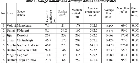
In the application for the evaluation of the identified patterns of stream flow and base flow was used data from gauging stations located in Moldavian Plain managed bu Prut-Bârlad Water Administration between 1981 and 2013. (Table 1). For the results to be more accurate were analyzed only gauging stations where leakage rivers is under natural conditions and in the basins supply upstream were not performed hydraulic works at large scale (reservoirs, catchments of water or derivatives rivers ).

Table 1. Gauge stations and drainage basins characteristics

No. River Gauge station D ist an ce t o co n fl u en ce (k m) Surface (km2)

Medium altitude (m) Average precipitation (mm) Average flow (m3_/s)

Max. flow (m3/s)

Min. flow (m3_/s)

1 VolovățManoleasa 7.0 214 178 502.1 0.455 69.0 0.001 2 Buhai Pădureni 8,0 54,2 165 592.5 0.171 96.0 0.001 3 Jijia Dorohoi 267 238 262 592.5 0.668 170.0 0.005 4 Sitna Cătămără ti 46,5 173 202 557.2 0.424 77.0 0.001 5 Miletin Nicolae Balcescu 46.0 220 202 641.0 0.470 226.0 0.001 6 Bahlui Vama cu Tabla 92.0 46 345 527.5 0.239 55.5 0.001 7 Magura Carjoaia 11.0 39 315 525.5 0.080 83.1 0.001 8 Bahluet Targu Frumos 23.5 68 252 491.4 0.187 95.0 0.001

*the valeus are corelated with the data obtained by Prut-Bârlad Water Administration

Moldavian Plain geological matrix consists in Sarmatian sedimentary deposits (clay, marl and sand) and quaternary deposits which has generated a relief with altitudes between 35 and 400 m. Quaternary loess clays is presented as an alluvial-colluvial deposits couverture, with 12-23 m thick deposited over pre-quaternary deposits eroded by the river Prut tributary river network (Dragomir, 2009). Geographical position, outside the Carpathian area creates a temperate climate with continental shades, where average annual temperatures vary between 8.5 and 9,50C and rainfall totals between 450 and 650 mm/year (Croitoru, Minea, 2014).

early October. Prolonged periods without precipitation are often more than 5 consecutive days, and sometimes over 10 consecutive days, causing that in the rivers flow, the underground supply to prevail over the surface supply and in general equation of flow Qi=Qb.

3. METHODOLOGY

To identify the most realible applied to cliamtic and geological conditions from the model aplicat lowland area from the north-eastern part of Romania was used several assessment models of BFI based on two methods: empirical methods based on hydrograph separation and filter based methods.

Hydrograph separation method it is the most applied method used in romanian hydrology. The results were correlated with climatic and geological condition of the drainage basin analyzed. For eastern part of Romania, Harjoabă, et al. (1997) calculates a BFI 0.68, for Moldavian Subcapathians and a BFI between 0.53 and 0.60, for Moldavian Plateau (Harjoaba, Amariucai, 1998).

Aplications of filter based methods involves the use of parameters identified by the statistical analysis of the data string. Of the models based on algorithms, in this paper was used local minimum method (LMM) used by Sloto and Crouse (1996), tooked over by Talaksen and van Lannen (2004) as emphirical methods based on daily flow hydrograph separation method. Within filter based methods was used Champan filter (1991), modified in in recursive digital filter (RDF) by using one parameter algorithm (Chapman and Maxwell, 1996), WHAT model (Lim et al., 2005) and Ekchardt filter (2008).

Initially the algorithm proposed by (1991 modified by Chapman and Maxwell, in 1996) turn to account just one parameter recession constant k:

Qbi=

Qbi-1+ Qi

Later models, like WHAT model (which is based on an algorithm

proposed by Ekchardt, in 2005) resumed and simplified in Ekchardt filter (2008)

Qbi

The filter parameter a can be analyzed on the basis of average daily flows taking into account the relationship: Qi-3>Qi-2>Qi-1>Qi>Qi+1>Qi+1, where Qi is taken

into account if there are at least 5 days with recession period. The a parameter values are determined by linear regression analysis based on the relationship Qi+1=f(Qi), taking into account only the recession period. After Nathan and

McMahon (1990), this parameter values generally fall between 0.9–0.95. For geological conditions in the north-eastern part of Romania the a parameter value was set at 0,925 (Minea et al., 2014).

4. RESULTS AND DISCUSSIONS

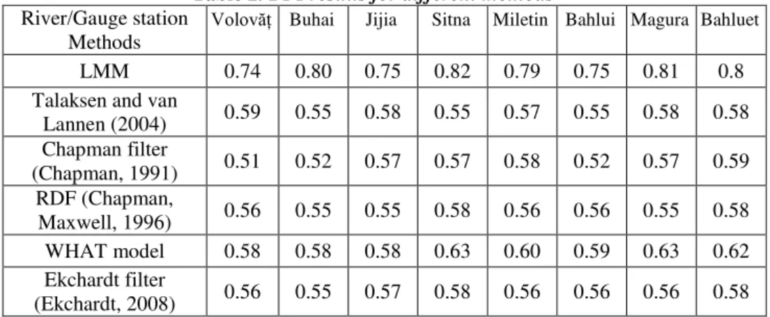
Applying the different methods used in assessing BFI showed that certain algorithms proposed by (1991) and Ekchardt (2008) give the best results in geographical conditions of the Moldavian Plain. Using local minimum method (LMM) very high values of BFI are obtained (over 0.75) which does not reflect the climate and geology realities of the area. The standard deviation values for this method do not exceed 0.15, and the coefficient of variation are over peste 0.22. Even if the average values of the precipitation amounts are reduced (in some places under 450 mm) the BFI not exceed 0.75, given that there is an increasing trend of precipitation in recent decades their (Croitoru, Minea, 2014).

Table 2. BFI results for different methods

River/Gauge station Methods

Volovăț Buhai Jijia Sitna Miletin Bahlui Magura Bahluet

LMM 0.74 0.80 0.75 0.82 0.79 0.75 0.81 0.8 Talaksen and van

Lannen (2004) 0.59 0.55 0.58 0.55 0.57 0.55 0.58 0.58 Chapman filter

(Chapman, 1991) 0.51 0.52 0.57 0.57 0.58 0.52 0.57 0.59 RDF (Chapman,

Maxwell, 1996) 0.56 0.55 0.55 0.58 0.56 0.56 0.55 0.58 WHAT model 0.58 0.58 0.58 0.63 0.60 0.59 0.63 0.62 Ekchardt filter

(Ekchardt, 2008) 0.56 0.55 0.57 0.58 0.56 0.56 0.56 0.58

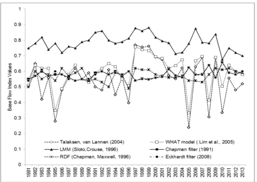
slight increase of BFI values in acording with increase in precipitation in this area in recent decades (Dumitrescu et al., 2014).

Fig. 1. BFI values variation between 1981-2013 using different methods in Moldavian Plain

Ekchardt (2008) suggest that there can be no real assessment base flow without being checked at least through other direct methods, as would be the tracer measurements. But considering the fact that the use of algorithms attenuates the peaks of base flow, conditioned by the intake of water from excess rainfall, reflected in the production of flood-basin, it can be considered that the data obtained by filter based methods are closer to reality (Figure 2). The correlation matrix between the different values of BFI obtained show that the best methods can be applied in this area are Chapman filter and Eckhardt filter (r=0.98). Both methods aim to identifying calculation parameters like a and BFI max which adjusted for this area (a=0.925, BFImax=0.7-0.8) indicates that the values of BFI exceeding 0.5.

If we take into account highly variable hydrological conditions during the year, and that over 35% of the river has a temporary drain (Minea, 2012), the BFI values according to the algorithm proposed by Eckhardt (2012) are the following:

- for basins developed on porous aquifer with perennial stream, asuming values for a=0.925 and BFI max=0.7, the values of BFI=0.55.

Fig. 2. Comparition between measured stremflow and calculated baseflow with Chapman and Ekchardt filters at the H.S. Targu Frumos (Bahluet)

5. CONCLUSIONS

Statistical modeling of BFI shows that the base flow in the stream flow for rivers that drain lowland area from north-eastern part of Romania is over 50%. These values are higher than the estimated values in studies in the years 70'-80 ', when base flow was considered as provide 15-35% of the total flow. The most realible models for this area is Chapman filter and Ekchardt filter, considering adjustment of statistical parameters depending on local climatic and geological conditions. The values of BFI obtained (over 0.5) suggest a careful reassessment of hydrological balances for the region, considering how land use changes and numerous hydraulic works carried out in recent decades.

REFERENCES

1. Anderson M.G., Burt T.P. (1980), Interpretation of recession flow. J. Hydrol., 46: 89-101.

2. Arnold J.G., Allen P.M., Muttiah R., Bernhard G. (1995), Automated base flow separation and recession analysis techniques, Ground Water, 33 (6): 1010-1018 3. Badea L, Gastescu P, Velcea VA and co-authors. (1983), Geography of Romania,

vol. 1, Geografia Fizica. Academy Press, Bucharest (in Romanian)

5. Chapman T.G., Maxwell A.I. (1996), Baseflow separation–Comparison of numerical methods with tracer experiments, Hydrological and Water Resources Symposium, Institution of Engineers Australia, Hobart, 539–545, 1996.

6. Croitoru A.E., Minea I. (2014), The impact of climate changes on rivers discharge in Eastern Romania, Theoretical and Applied Climatology, DOI 10.1007/s00704-014-1194-z2012.

7. Diaconu C. (1971), Rivers of Romania, I.M.H. Press, Bucharest (in Romanian). 8. Dragomir S. (2009), Geochemistry on the undergorundwater from Iasi Conty,

Al.I.Cuza Univ. Press, Iasi 298p. (in romanian).

9. Dumitrescu A., Bojariu R., Bîrsan M.V., Marin L., Manea A. (2014), Recent climatic changes in Romania from observational data (1961–2013), Theoretical and applied climatology, DOI 10.1007/s00704-014-1290-0

10. Eckhardt K. (2005), How to construct recursive digital filters for base flow separation, Hydrological processes, 19: 507-515,

11. Eckhardt K. (2008) A comparition of baseflow indices, which were calculated with several different base flow separation methods, Journal of Hydrology, 352: 168-173.

12. Eckhardt K. (2012, Technical Note: Analytical sensitivity analysis of a two parameter recursive digital base flow separation filter, Hydrol. Earth Syst. Sci., 16:451–455.

13. Hârjoabă I., Amăriucăi M., Olariu P. (1997), Consideration sur les raports

existant entre les sources d’alimentation de surface et souterraine dans les bassins

des rivieres Asau et Tutova, An. t Univ. Al.I.Cuza, tom XLII-XLIII, s II-c, Geografie: 26-35.

14. Hârjoabă I., Amăriucăi M. (1998) Ratio between streamflow (S) and baseflow (U) in Bahluet drainage basin, Lucr. Sem.Geogr. „Dimitrie Cantemir”, nr.15-16: 69-74 (in romanian)

15. Institute of Hydrology (1980), Low Flow Studies report. Wallingford, UK. 16. James L.D., Thompson W.O. (1970), Least squares estimation of constants in a

linear recession model, Water Resour. Res., 6(4): 1062-1069.

17. Lim K.J., Engel B.A., Tang Z., Choi J., Kim K.S., Muthukrishnan S., Tripathy D. (2005), Automated web gis based hydrograph analysis tool, WHAT, J American Water Resour. Assoc.: 1407-1416.

18. Lyne, V.D., Hollick M. (1979), Stochastic Time-Variable Rainfall Runoff Modeling, Hydrology and Water Resources Symposium; Institution of Engineers: Perth, Australia: 89–92.

19. Minea I. (2010), Minimum discharge in Bahlui basin and associated hydrologic risks, Aerul şi apa componente ale mediului, Presa Universitară Clujeană Press: 508-515.

20. Minea I., (2012), Bahlui draiange basin – hydrological study, Al.I.Cuza Univ. Press, Ia i, pp 333. (in romanian)

21. Minea I., Mihu-Pintilie A, Iosub M., Hapciuc O.E. (2014), Preliminary evaluation on the ratio between the surface and underground river supply in eastern Romania, Aerul şi apa componente ale mediului, Presa Universitară Clujeană Press: 150-156

22. Nash J.E. (1966), Applied flood hydrology. In: R.B. Thorn (Editor), River Engineering and Water Conservation Works. Butterworths, London: 63-110. 23. Nathan R.J., McMahon T.A. (1990), Evaluation of automated techniques for

24. Piggott A.R., Moin S., Southam C. (2005). A revised approach to the UKIH method for the calculation of Base flow, Hydrol. Science J, 50:911-920.

25. Rutledge A.T. (1998), Computer programs for describing the recession of groundwater discharge and for estimating mean groundwater recharge and discharge from streamflow data, USGS Water Resources Investigations Report 98-4148, 43 p.

26. Sloto R.A., Crouse M.Y. (1996), HYSEP: A Computer Program for Streamflow Hydrograph Separation and Analysis; U.S. Geological Survey Water-Resources Investigations Report 96-4040; U.S. Geological Survey: Denver, CO, USA, 1996; pp. 46.

27. Sorocovschi V. (1996), Târnavelor Plateau– hydrological study, Cetib Press, Cluj-Napoca, 191 pp. (in Romanian).

28. Talaksen L.M., van Lannen H.A.J. (2004), Hydrological drought: processes and estimation methods for streamflow and groundwater, Elsevier, Developments in water science (48), 581 p.