Land Surface Model and Particle Swarm
Optimization Algorithm Based on the
Model-Optimization Method for Improving Soil
Moisture Simulation in a Semi-Arid Region
Qidong Yang1*, Hongchao Zuo2, Weidong Li1
1Department of Atmospheric Sciences, Yunnan University, Kunming, Yunnan Province, China,2College of Atmospheric Sciences, Lanzhou University, Lanzhou, Gansu Province, China
Abstract
Improving the capability of land-surface process models to simulate soil moisture assists in better understanding the atmosphere-land interaction. In semi-arid regions, due to limited near-surface observational data and large errors in large-scale parameters obtained by the remote sensing method, there exist uncertainties in land surface parameters, which can cause large offsets between the simulated results of land-surface process models and the observational data for the soil moisture. In this study, observational data from the Semi-Arid Climate Observatory and Laboratory (SACOL) station in the semi-arid loess plateau of China were divided into three datasets: summer, autumn, and summer-autumn. By combing the particle swarm optimization (PSO) algorithm and the land-surface process model SHAW (Simultaneous Heat and Water), the soil and vegetation parameters that are related to the soil moisture but difficult to obtain by observations are optimized using three datasets. On this basis, the SHAW model was run with the optimized parameters to simulate the char-acteristics of the land-surface process in the semi-arid loess plateau. Simultaneously, the default SHAW model was run with the same atmospheric forcing as a comparison test. Sim-ulation results revealed the following: parameters optimized by the particle swarm optimiza-tion algorithm in all simulaoptimiza-tion tests improved simulaoptimiza-tions of the soil moisture and latent heat flux; differences between simulated results and observational data are clearly reduced, but simulation tests involving the adoption of optimized parameters cannot simultaneously improve the simulation results for the net radiation, sensible heat flux, and soil temperature. Optimized soil and vegetation parameters based on different datasets have the same order of magnitude but are not identical; soil parameters only vary to a small degree, but the varia-tion range of vegetavaria-tion parameters is large.
OPEN ACCESS
Citation:Yang Q, Zuo H, Li W (2016) Land Surface Model and Particle Swarm Optimization Algorithm Based on the Model-Optimization Method for Improving Soil Moisture Simulation in a Semi-Arid Region. PLoS ONE 11(3): e0151576. doi:10.1371/ journal.pone.0151576
Editor:Yong Deng, Southwest University, CHINA
Received:November 4, 2015
Accepted:March 1, 2016
Published:March 18, 2016
Copyright:© 2016 Yang et al. This is an open access article distributed under the terms of the Creative Commons Attribution License, which permits unrestricted use, distribution, and reproduction in any medium, provided the original author and source are credited.
Data Availability Statement:Data are from the Semi-Arid Climate Observatory and Laboratory (SACOL) station, a study whose authors may be contacted athttp://climate.lzu.edu.cn/english/index. asp.
Introduction
Soil moisture is an important component of global energy and water circulation. The soil mois-ture can directly affect meteorological and hydrological processes by affecting physical pro-cesses such as surface evaporation, vegetation transpiration, and runoffs [1,2,3,4] and can indirectly affect the global carbon circulation by affecting vegetation growth and plant photo-synthesis [5,6,7,8,9]. Thus, accurately observing and simulating the soil moisture is critical for studying global climate change [10,11]. However, the spatial and temporal inhomogeneity of the soil moisture distribution causes great difficulties in its observation and simulation. On one hand, although techniques such as time domain reflectometry (TDR) can be used to observe the soil moisture at stations [12], it is difficult to obtain high-precision, large-scale, and long-term observational data. On the other hand, although extant land-surface process models or climate models can be used to simulate long-term variation trends of the soil moisture, there exist large offsets between simulated results and observational data [13]. Furthermore, different results are obtained by using different models [14,15,16]; consequently, it is difficult to estab-lish reliable global soil moisture datasets through model simulations. Thus, it is of significant importance to improve the capability of land-surface models to simulate the soil moisture and thereby improve numerical weather forecast and climate predictions.
Generally, the simulation capability of a land-surface process model is closely related to the parameterization schemes and input parameters of the model [14]. The parameterization schemes adopted in a model is built based on field observational data; therefore, different mod-els adopt different parameterization schemes for plants and soil. Comparisons of multiple land-surface process models have indicated that different land-surface parameterization schemes have a significant impact on the simulation results [15,17,18]. Based on the actual land-surface condition, an appropriate parameterization schemes can improve the simulation capability. In addition, land-surface process models require the input of multiple parameters for simulation, including vegetation and soil parameters, terrain parameters, and the initial soil hydrothermal conditions. These parameters significantly affect the simulation results
[19,20,21]. Some of these parameters can be obtained with high precisions by station or remote-sensing observations. For instance, the soil content, vegetation root distribution, sur-face aerodynamic roughness, and initial soil temperature can be obtained by station observa-tion. By contrast, the vegetation leaf area index, vegetation height, and surface albedo can be measured by large-scale remote sensing. However, it is difficult (if not impossible) to observe some parameters for the following reasons: (1) Values obtained by station observation cannot represent values on a large scale. Because certain parameters, such as the saturated soil water conductivity, vary at different locations, the observed value at one point cannot be used for its neighboring point; (2) Some parameters can be interactively connected, and it is difficult to precisely measure all of them together, for example, the empirical parameter of vegetation tran-spiration stomatal resistance; (3) Some parameters used in a model do not have definitive phys-ical meaning and therefore cannot be observed, for example, the Clapp-Hornberger constant. To overcome these difficulties, different combinations of land-surface parameters are used in a model, and by comparing differences between simulation results and observational data, the adaptability of model parameters can be evaluated, which is known as the parameter calibra-tion process. Multiple studies have demonstrated that the simulacalibra-tion capability of land-surface process models can be improved by calibrating adopted parameters [22,23].
In the past 20 years, intelligent or optimized algorithms have attracted wide interest with respect to calibrating land-surface models. For instance, the SCE(Shuffled Complex Evolution) global optimization method has been used to calibrate the hydrological model [24]; Gupta et al. adopted multicriteria methods for parameter estimation, which (1) proves effective when analysis, decision to publish, or preparation of the
manuscript.
only the range of parameter physical values is known and (2) can improve the simulation capa-bility of the BATS(Biosphere-Atmosphere Transfer Scheme) model [25]. In addition, to assim-ilate the soil moisture, Ines et al. also used the genetic algorithm to estimate hydrological parameters [26]. In recent years, another optimization algorithm, particle swarm optimization, has become popular [27] and has been widely applied in other research areas [28]. This algo-rithm was built on the basis of animal behaviors, such as the process of searching for food by fish or birds, which essentially is a particle constrained by a certain object function solving a global (or approximately global) optimal solution. Calibrating parameters in land-surface pro-cess models is a similar propro-cess, i.e., choosing different parameter combination methods to reduce the difference between observational and simulation results during a certain period. Thus, many researchers have used particle swarm optimization to optimize parameters for hydrological models. For example, Gill et al. used the multiple-objective particle swarm optimi-zation to estimate hydrological parameters [29]; Chaw et al. used the particle swarm optimiza-tion method to predict the water level by combining ANNs(Artificial Neural Networks)[30]; Scheerlinck compared the similarity and difference in optimizing model parameters between the MWAPRE(Multistart Weight-adaptive Recursive Parameter Estimation) and particle swarm optimization algorithms and found that the particle swarm optimization algorithm is more practical and more effective in utilizing observational data [31]; Zhang et al. evaluated the pros and cons of five optimization methods in calibrating hydrological models [32] and found that compared with other methods, particle swarm optimization can be used to obtain the optimal parameter solution, which also takes less time.
The semi-arid region is approximately 40% of the global land surface [33]. Its surface types are mainly composed of sparse vegetation, grassland, and desert, whose surface characteristics significantly differ from that of the humid region [34]. In addition, the semi-arid region is sen-sitive to climate change and has the highest variability in precipitation [35]. Therefore, the eco-logical and water-resource systems in the semi-arid region are closely related to the soil moisture [9,36]. Vegetation destruction and grassland desertification caused by human activi-ties can further cause an anomalous change in the soil moisture, resulting in negative feedback of the climate system and consequently threatening the human living environment
[9,36,37,38]. Due to the lack of knowledge regarding the specific characteristics of the land-sur-face process in semi-arid regions, limited near-surland-sur-face observational experiments, and large offsets in large-scale parameters obtained by the remote-sensing method, land-surface process models have a low simulation capability [39]. Thus, conducting comprehensive near-surface observation experiments, accurately identifying land-surface parameters or parameter combi-nations using optimized methods are critical for improving the soil moisture simulation capa-bility in semi-arid regions. However, several limitations and difficulties still exist in former studies. (1) A complete land surface process model contains the vegetation, soil, snow and atmospheric boundary layer, involving many parameters which are dependent. But in the exist-ing study, most of the optimization algorithms only used for simple or simplified hydrological model [26,29,31], therefore, the optimized parameters can not be applied in complete models. (2) In previous studies, the optimization parameters were selected arbitrarily and the related physical processes were not considered [25]. The dimension of the optimization parameters space was too high and the parameters combinations were too many. Hence, the optimized parameters combinations cannot be used in models. For example, all the input parameters were selected for optimization. (3) In previous studies, optimized parameters were usually obtained by a single and short length dataset. Correspondingly, the optimized parameters are not accurate for longtime simulation.
China and divided the data into different datasets. By adopting the particle swarm optimization method, this study optimizes soil and vegetation parameters related to soil moisture in the land-surface process model, SHAW (Simultaneous Heat and Water). On this basis, the opti-mized parameters are utilized in the SHAW model to improve the capability of the SHAW model to simulate the soil moisture in the semi-arid region.
Methodology
SHAW Model
The SHAW model was developed by Flerchinger et al [40,41] and was initially used to simulate the freezing and melting of soil. After continuous development and improvement, SHAW gradually forms a comprehensive land-surface model, which includes interactions between soil, the accumulated snow-residue layer, vegetation, and atmosphere. The SHAW model can divide the vegetation and residue into less than 10 layers, the accumulated snow into less than 100 layers, and the soil into less than 50 layers. In addition, the model considers radiation transfer, convective exchange, hydrothermal transport in soil, precipitation infiltration, and soil freeze-up and melt between different physical layers. The SHAW model is a single-point land surface model, most of the vegetation and soil parameters can be directly observed based on the actual underlying conditions. Only a few of input parameters in the SHAW model which need optimize are difficult to observe. The dimension of optimized parameters space is low. Most of the input parameters in SHAW model can be easily transferred to other land sur-face models. The model has been applied to simulation studies on different underlying sursur-faces. A series of tests have been conducted for complicated underlying surfaces in the semi-arid region [40,42].
The controlling equation of the soil moisture in the SHAW model can be expressed as [43]:
@yl @t þ
ri rl
@yi @t ¼
@ @z½Kð
@c
@z þ1Þ þ
1 rl
@qv
@z þU ð1Þ
in which,zrepresents the soil depth (m),trepresents time (s),θl(θi) represents the soil
volu-metric water (ice) content (m3m-3),ρl(ρi) represents the water (ice) density (kg m-3),K
repre-sents the water conductivity (m s-1),ψrepresents the soil water potential (m),qvrepresents the
soil water vapor density (kg m s-1) (which is determined by the soil volumetric water content), andUrepresents the vegetation root water absorption (m3m-3s-1).
The soil water potentialψand water conductivity can be calculated using the following equation:
c¼ceðyl ysÞ
b
ð2Þ
K¼Ksð yl ysÞ
ð2bþ3Þ
ð3Þ
in whichψeis the air entry potential (m),bis the Clapp-Hornberger constant,θsis the saturated
water content (m3m-3), andKsis the water conductivity when the soil is saturated (m s-1).
The vegetation root water absorptionUdepends mainly on the vegetation transpiration, which is determined by the soil-vegetation-air water transport and can be expressed as:
Tj¼
XNS
k¼1
ck cx;j
rr;j;k
¼X
NC
i¼1
cx;j cl;i;j
rl;i;j
¼X
NC
i¼1
rvs;i;j rv;i
rs;i;jþrh;i;j
in whichiis the canopy,jis the number of plant species,kis the soil layer,NCis the total num-ber of the canopy layers,NSis the total number of the soil layers,Tjis the total transpiration
(kg m-2s-1),Li,jis the leaf surface area index,ρvs,i,jandρv,iare the water vapor densities of the
leaf surface and of the air inside the canopy, respectively (kg m-3),ψx,jandψl,i,jare the water
potentials of the vegetation xylem and of the leaf, respectively (m),rhandrsare canopy air and
stomatal resistances, respectively, (s m-1), andrlandrrare leaf and root resistances, respectively
(m3s kg-1), which can be expressed as:
rh¼307ðdl=uÞ
1=2
ð5Þ
rs¼rso½1þ ðcl=ccÞ
5
ð6Þ
rl ¼rloðLi=LÞ ð7Þ
rr¼rroðDp;i=DpÞ ð8Þ
in whichdlis the Characteristic dimension of the leaves(m),uis the wind speed within the
can-opy (m s-1),rsois the minimal stomatal resistance (s m-1),rloandrroare the leaf and root
resis-tance constants, respectively (m3s kg-1),ψcis the critical leaf water potential, andL(Li) and Dp(Dp,i) are the total leaf surface area (the leaf surface area of each layer) and total root ratio
(the root ratio of each layer), respectively.
For the soil-moisture controlling equation described above, its upper boundary condition can be expressed as:
qs¼P Es Rs ð9Þ
in whichqsis the waterflux that enters the soil (m s-1),Pis the precipitation rate or melting
rate of accumulated snow (m s-1),Esis the evaporation of the soil surface (m s-1), andRs
repre-sents surface runoffs (m s-1).
In the lower boundary condition of the soil moisture, the gradient of the soil moisture is set at zero. Finally, land-surface process models must also satisfy the energy balance equation, which is:
Rn¼HþLvEþG ð10Þ
in whichGis the soil heatflux (W m-2),Rnis the net radiation (W m-2),His the sensible heat
flux (W m-2),Eis the water vaporflux (kg m-2s-1), andLvis the potential evaporation coeffi
-cient. The method above used to parameterize factors related to the soil moisture shows that all of the vegetation and soil parameters (includingψe,b,θs,Ks,rso,rlo,rro,ψc,dl,L, andDp) can
affect simulations of the soil moisture.
PSO Algorithm
If we want to optimize ann-dimensional problem formparticles, the position and velocity vector of theithparticle can be expressed as:
xi ¼ ðxi1;xi2;. . .;xinÞ ð11Þ
vi¼ ðvi1;vi2;. . .;vinÞ ð12Þ
The updated position and velocity of the ithparticle can be expressed as:
vNþ1
in ¼ov N
inþc1r1ðp N in x
N
inÞ þc2r2ðG N n x
N
inÞ ð13Þ
xNþ1
in ¼x N in v
N
in ð14Þ
in whichNrepresents the number of iterations;wrepresents the inertia weight;c1andc2are
the acceleration constants, which are the weight coefficients of the optimal value by tracking its own history and therefore represent self-awareness of the particle;r1andr2are random
num-bers in [0,1].piandGnrepresent the optimal value of theithparticle by searching its history and the optimal position searched by all the particles, respectively, which can be expressed as:
pi ¼ ðpi1;pi2;. . .;pinÞ ð15Þ
Gn¼ ðpg1;pg2;. . .;pgnÞ ð16Þ
g¼min
1in½fðpiÞ ð17Þ
in whichgrepresents the position when the value of the object function is the lowest andfis the object function. The object functionfin the PSO algorithm can be a single function or vec-tor function. Whenfis a vector function, it should be the multiple object function; therefore, one method is to solve for its Pareto front, and another method, proposed by Crow et al.[45], is to standardize multiple variables with different orders of magnitude and then define a single object function to solve for its minimum.
Data and Method
Data
Model-optimization Method
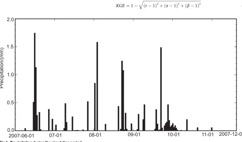
To run land-surface process models, input variables include the atmospheric forcing condition, the initial condition for the soil temperature and moisture, and surface vegetation and soil parameters. In this study, the simulation period is set to the summer and fall seasons of 2007 (from 01/06 to 30/11) to avoid the effect of snow. According to the actual underlying surface condition, we divide the vegetation into one layer and the soil into six layers of 5, 10, 20, 40, 80, and 250 m, which is consistent with the observational depths. The atmospheric forcing variable adopts the hourly wind speed, temperature, pressure, precipitation, relative humidity, down-ward short-wavelength radiation, and downdown-ward long-wavelength radiation at the SACOL sta-tion. The soil moisture is mainly affected by the precipitation; therefore precipitation during the simulation period is show inFig 1.
The initial conditions of the soil temperature and moisture are taken from the actual obser-vational data on 01/06/2007. If a surface parameter can be directly observed, then the observa-tional value is adopted in the model; if a parameter is difficult to observe, it is then solved for its optimal value or parameter combination using the particle swarm algorithm. According to the parameterization schemes for the soil moisture in the SHAW model discussed above, we choseψe,b,θs,Ks,rso,rlo,rro, andψcas the parameters for optimization. Because the soil layer is
divided into six layers, there are 16 parameters in total by assuming that theψe,b,θs,Ksvalues
of adjacent layers are the same.
When utilizing the PSO algorithm to optimize parameters, an object function must be defined. In this study, the Kling-Gupta efficiency (KGE) function proposed by Gupta et al is used as the object function, which is defined as [47]:
KGE¼1
ffiffiffiffiffiffiffiffiffiffiffiffiffiffiffiffiffiffiffiffiffiffiffiffiffiffiffiffiffiffiffiffiffiffiffiffiffiffiffiffiffiffiffiffiffiffiffiffiffiffiffiffiffiffiffiffiffiffiffiffi
ðr 1Þ2þ ða 1Þ2þ ðb 1Þ2
q
ð18Þ
Fig 1. Precipitation during the simulation period.
in whichrrepresents the correlation coefficient between the observational and simulation value,αrepresents the ratio of the standard deviation of the observational value to that of the simulation value, andβrepresents the ratio of the mean observational value to the mean simu-lation value. KGE is used to evaluate the quality of thefit for the simulation result with the observation, whose range varies from -1to 1; the closer the value is to 1, the better the simula-tion capability. CorrespondingKGEj(j represents the corresponding soil moisture,
tempera-ture, etc.) values are calculated using the soil moistempera-ture, surface temperatempera-ture, sensible heatflux, latent heatflux, net radiation, and corresponding observational values of thefive-layers soil simulated by the SHAW model. Thefinal KGE is the average of allKGEjvalues. Because all
these variables have different orders of magnitude, they are standardized during the calculation of both simulation and observation, i.e., the corresponding average value is subtracted from each observational or simulation value, which is then divided by the corresponding standard deviation [31].
The PSO algorithm also depends on parameters of the model itself, specifically, the number of particle swarm,N,c1, c2, w, and the position and velocity variation range of each particle.
According to multiple simulation tests and previous studies [29,31], (1) n = 20; (2)N= 300; (3) the variation range of w is from 0.2 to 0.5; (4)c1= 1.7, andc2= 2; (5) the variation range of the
particle position is from -1 to 1, and that of the particle velocity is from -0.01 to 0.01. For all parameters that must be optimized, their variation ranges become [–1,1] by the following method:
x¼2y ðRmaxþRminÞ
ðRmax RminÞ
ð19Þ
in whichyis the actual value of a parameter for optimization andRmaxandRminrepresent the
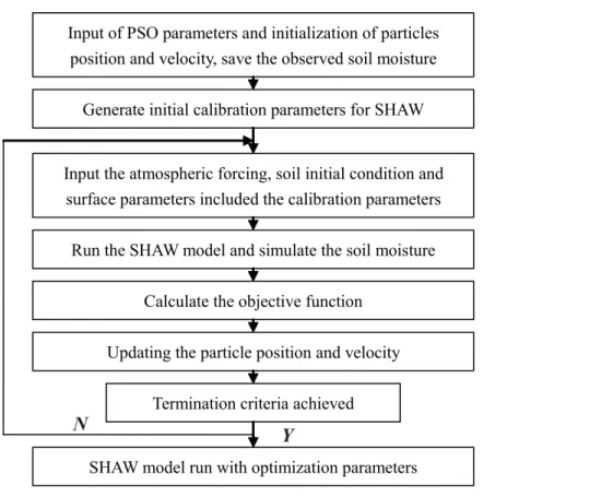
range of the parameter for optimization. Based on the process described above, the combina-tion of the SHAW model and the PSO algorithm is called the SHAW_PSO method. The detailed realization method is depicted in the followingflow chart (Fig 2).
To optimize parameters, the datasets are divided into three groups: the first group consists of summer (June-August) data, the second group consists of autumn (September-November) data, and the third group consists of data from the summer-autumn (June-November) period, which are used for separate parameter optimization. The results of the SHAW model obtained by adopting the optimized parameters are tested against all the summer and autumn data, which are recorded as“SHAW_PSO_SU”,“SHAW_PSO_AU”, and“SHAW_PSO_SA”. As a control test, the model was also run with the same atmospheric forcing variables, the initial condition, and the default parameters of the model given inTable 1, named“SHAW_DEFAULT”. In
Results
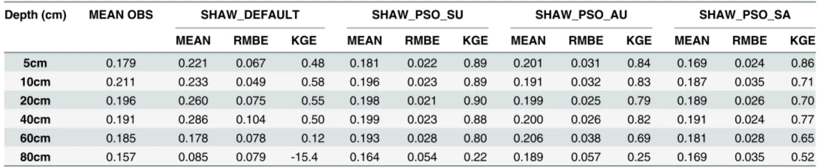
Fig 3a–3eshows the comparison of soil moisture (SM) values simulated by the four sets of sim-ulation tests with the observational data. As presented in theFig 3, all the simulation results after parameter optimization can reasonably reproduce the variation trend of the soil moisture, but the SHAW_DEFAULT test cannot predict the variation trend below 40 cm, indicating that the soil and vegetation parameters suggested by the model differ from the actual underlying surface.Table 2lists the root-mean-square deviation and the KGE value of the simulated results with respect to the measured data, which clearly illustrate that offsets of the simulation tests are all reduced after parameter optimization relative to that of the SHAW_DEFAULT test; their corresponding KGE values are also increased, which demonstrates that parameter optimization significantly improves the model’s simulation capability. By comparing the three sets of simulation tests after parameter optimization, we can observe that the soil moistures of all the layers above 80 cm simulated by SHAW_PSO_SU are closer to the measured data than are the values from the other two simulation tests. The deep soil moisture is related to the underground water. The SHAW model does not contain the underground water parameteriza-tion scheme. Hence, the absence of the underground water parameterizaparameteriza-tion may also affect the soil moisture simulation.
Fig 4shows the scatter plots of the net radiation, sensible heat and latent heat fluxes, and soil temperature at 5 cm calculated by different sets of simulation tests, compared with the cor-responding observational data.Table 3lists the corresponding offsets, average values, and KGE values of different simulation tests. As shown in the figure, the simulations of net radiation(Fig 4a1–4a4) produced by different sets of model tests are all close to the observational data, which
Fig 2. SHAW-PSO method flow chart.
can be demonstrated by the close to 1:1 linear fit lines with correlation coefficients all above 0.99. The offsets given inTable 3indicate that the net radiation simulated by SHAW_PSO_AU is the closest to the observational data with the highest KGE. The correlation coefficients between the simulated sensible heat flux values (Fig 4b1–4b4) and the observational data are all high (>0.85), but all of the simulated values are higher than the observational data.Table 4
shows that the offset between the sensible heat flux and the observational data is the smallest for the simulation by SHAW_DEFAULT. The correlation coefficients of the latent heat flux (Fig 4c1–4c4) values simulated by different sets of simulation tests and the observational value are all above 0.75, and the model tests with optimized parameters all have improved simulation results for the latent heat flux relative to SHAW_DEFAULT. In particular, the latent heat flux simulated by SHAW_PSO_SA agrees the best with observation and has the highest KGE. The correlation coefficients between the simulation results of different model tests and the observa-tional data for the soil temperature (Fig 4d1–4d4) are all above 0.94, and the linear fit lines are close to the 1:1 line; the soil temperature simulated by SHAW_PSO_SU is most consistent with the observation. Based on analysis of the net flux, sensible heat and latent heat fluxes, and soil temperature, we can observe that the simulation capabilities for the latent heat flux in different tests are all improved, but the simulation results for all of the subcomponents cannot be improved simultaneously. This finding is similar to the Pareto front yielded by the multiple object function method [22]. Previous studies by Gupta et al have also indicated that the adop-tion of optimized parameters cannot improve the simulaadop-tion capabilities for all the variables in
Table 1. Input parameters for the SHAW-PSO model.
Variable Symbol Default Unit Range
Vegetation parameters
Plant albedo αc 0.23 - -
-Transpiration temperature Tc 7 K
-Minimum stomatal resistance rso 100 m s-1 [10,1000]
Critical leaf water potential ψc -100 m [-10,-1000]
Leaf resistance rlo 1e5 m3s kg-1 [1e4,1e6]
Root resistance rro 2e5 m3s kg-1 [2e4,2e6]
Plant height H 0.15 m
-Characteristic dimension of the leaves dl 5e-3 m
-Dry biomass Wg 0.5 kg m-2
-Leaf area index L 1.5 - -
-Effective rooting depth Dp 0.15 m
-Soil parameters
Air-entry potential ψe -0.31 m [-1.0,-0.1]
Campbell’s pore-size index b 4.5 - - [3,10]
Saturated conductivity Ks 2e-6 m s-1 [5e-5,5e-7]
Saturated volumetric moisture content θs 0.43 - - [0.3,0.6]
Bulk density ρb 1020 kg m-3
-Sand percent sand% 38 %
-Silt percent silt% 26 %
-Clay percent clay% 22 %
-Organic percent om% 14 %
-Dry soil albedo αs 0.30 - -
-Exponent for the calculated albedo a -2 - -
-Aerodynamic roughness zom 0.46 - -
Fig 3. Comparison of the soil moistures calculated by different sets of simulation tests with the observational values.(a) 5cm (b) 10cm (c)20cm (d)40cm (e)80cm.
land-surface process models [25]. In addition, the large offsets of simulation results for the sen-sible and latent heat fluxes are perhaps related to the energy closure degree in this region. Previ-ous relevant studies have demonstrated that the average energy closure degree in this region is approximately 0.75 [50]. In this study, the energy closure in summer and autumn is 0.78 and 0.77. Because the SHAW model is built on the basis of the energy closure, it necessarily results in offsets in the simulation results relative to the observational data, thereby revealing that the simulation capability of a model is related to the model structure, the parameterization schemes adopted in the model, and the energy closure degree during observation.
Table 4summarizes parameters optimized based upon different datasets. The table reveals that the different sets of parameters are not identical, whereas they all have the same order of magnitude. The parameters related to soil (ψe,b,θs, andKs) optimized by using different
data-sets are consistent with small variation ranges, whereas the parameters related to vegetation (rso,rlo,rroandψc) all vary to large degrees, which might be related to the underlying surface
condition: the soil parameters only slightly vary with changing seasons, whereas the vegetation parameters are strongly dependent on seasons. Thus, in land-surface process models, it is more appropriate to set the vegetation parameters as time-dependent variables.
Conclusions and Discussion
Soil moisture is an important component in energy and water circulations. For simulation studies on climate, it is crucial to accurately simulate soil moisture. However, there still exist large offsets in current land-surface process models, which are coupled with climate models via land-surface process models and therefore cause uncertainties in the simulation results of weather and climate models. Thus, it is critical to accurately observe and simulate soil moisture. The semi-arid region is a belt that is sensitive to climate change, and variation in the soil mois-ture is of great importance to the regional climate. Because of the lack of knowledge regarding the specialty of the land-surface process in semi-arid regions, limited near-surface observa-tional experiments, and large offsets in large-scale parameters obtained by the remote sensing method, there are large deviations of the simulated soil moisture from the observational data. To improve the capability of land-surface process models to simulate soil moisture in semi-arid regions, we adopted the PSO algorithm and data from the SACOL station in the semi-semi-arid loess plateau to be used for comparison with the simulation results of the SHAW model with optimized soil and vegetation parameters and obtained following conclusions:
1. Different simulation tests of the SHAW model optimized by the PSO algorithm based on different datasets can all significantly improve simulations for the soil moisture and latent heat flux. In particular, the SHAW_PSO_SU model results agree the best with the observa-tional data for soil moisture above 80 cm (with the highest KGE value), whereas the latent
Table 2. Root mean square error and the KGE value of the simulated soil moisture at different depths.
Depth (cm) MEAN OBS SHAW_DEFAULT SHAW_PSO_SU SHAW_PSO_AU SHAW_PSO_SA
MEAN RMBE KGE MEAN RMBE KGE MEAN RMBE KGE MEAN RMBE KGE
5cm 0.179 0.221 0.067 0.48 0.181 0.022 0.89 0.201 0.031 0.84 0.169 0.024 0.86
10cm 0.211 0.233 0.049 0.58 0.196 0.023 0.89 0.191 0.032 0.83 0.187 0.035 0.71
20cm 0.196 0.260 0.075 0.55 0.198 0.021 0.90 0.199 0.025 0.79 0.189 0.026 0.70
40cm 0.191 0.286 0.104 0.50 0.199 0.023 0.88 0.200 0.026 0.82 0.191 0.024 0.77
60cm 0.185 0.178 0.078 0.12 0.193 0.028 0.80 0.206 0.038 0.69 0.181 0.028 0.65
80cm 0.157 0.085 0.079 -15.4 0.164 0.054 0.22 0.189 0.057 0.25 0.169 0.035 0.52
heat flux simulated by the SHAW_PSO_SA model shows minimal deviation from the observational data (with the highest KGE value). These improvements indicate that after optimization of parameters related to soil moisture, the simulation capability of the SHAW model for soil moisture and latent heat flux is improved.
2. The optimized SHAW model cannot well simulate the net radiation, sensible heat flux, and soil temperature simultaneously. In particular, the net radiation simulated by SHAW_PSO_AU shows the smallest offset from the observational data, which also has the highest KGE value. In
Fig 4. Scatter plots of the net radiation, sensible and latent heat fluxes, and soil temperature relative to the corresponding observational data in different sets of simulation tests.(a1-a4) Radiation (b1-b4) Sensible heat flux (c1-c4) Latent heat flux (d1-d4) Soil temperature at 5cm depth.
addition, the sensible heat flux calculated by SHAW_DEFAULT agrees the best with observa-tion and has the highest KGE value. Finally, the soil temperature simulated by SHAW_P-SO_SU is most consistent with observation and has the highest KGE value. These results indicate that the simulation capability of a model is not only related to input parameters but also depends strongly on the model structure, the parameterization schemes, and the energy closure degree during observation.
3. The soil and vegetation parameters are not identical among optimizations based on differ-ent datasets, but all have the same order of magnitude. The varying range of parameters related to soil is limited, whereas that related to vegetation is large, which might be associ-ated with the characteristics of the underlying surface. For instance, soil parameters vary with the season to a small degree, whereas vegetation parameters significantly change with seasons. Thus, it is more appropriate to set vegetation parameters as time-dependent vari-ables in land-surface process models.
Our study showed that the SHAW model, by adopting parameters related to the soil mois-ture optimized by the PSO algorithm, can improve the simulation capability for soil moismois-ture. In simulation studies, there still exist a few problems in using the PSO algorithm or other opti-mization algorithms, which must be addressed in future studies, as follows: (1) Parameters obtained by an optimization algorithm should be further tested against observations. Although optimized parameters or parameter combinations can improve the simulation capability of land-surface process models, some of these parameters have specific physical meanings. Thus, optimized parameters must satisfy their corresponding physical variation ranges and therefore cannot be only mathematically treated as the optimal solutions; (2) The dimension of a param-eter for optimization cannot be too high. There is a limit; in fact, the higher the dimension is, the more corresponding combination methods for the parameters and, in turn, the larger the variation ranges of the optimized parameters. Thus, in practice, observation and optimization algorithms should be complementarily combined: if a parameter can be observed, the observa-tional value should be used; for parameters that are difficult to observe, an optimization algo-rithm should be adopted; (3) The simulation test results in this study showed that soil moisture
Table 3. Root mean square error and the KGE value of the simulated net radiation, sensible, latent heat flux and soil temperature.
Variable MEAN OBS SHAW_DEFAULT SHAW_PSO_SU SHAW_PSO_AU SHAW_PSO_SA
MEAN RMBE KGE MEAN RMBE KGE MEAN RMBE KGE MEAN RMBE KGE
Rn 99.17 108.35 25.11 0.89 108.47 25.51 0.89 105.65 21.43 0.92 106.37 22.25 0.91
Sen 22.63 38.44 59.39 0.36 41.92 63.26 0.32 47.34 70.28 0.25 45.26 68.52 0.27
Lat 41.49 47.01 51.38 0.65 46.27 47.61 0.71 34.62 47.78 0.67 39.52 46.11 0.75
Tg 15.27 16.36 3.37 0.84 15.44 3.00 0.89 16.62 3.58 0.82 15.96 3.15 0.86
doi:10.1371/journal.pone.0151576.t003
Table 4. Parameters optimized based upon different datasets.
variables rso ψc rlo rro ψe,1 ψe,2 ψe,3 θs,1 θs,2 θs,3 Ks,1 Ks,2 Ks,3 b1 b2 b3
m s-1 m m3s kg-1 m3s kg-1 m m m m3m-3 m3m-3 m3m-3 m s-1 m s-1 m s-1 - - - -
-SHAW_PSO_SU 205 -365 6.85e5 1.49e6 -0.58 -0.49 -0.15 0.37 0.35 0.43 2.86e-6 3.63e-6 2.68e-6 4.82 4.72 6.22 SHAW_PSO_AU 401 -268 3.45e5 1.64e6 -0.92 -0.68 -0.62 0.40 0.39 0.37 2.50e-6 3.43e-6 4.08e-6 6.31 7.92 5.98 SHAW_PSO_SA 328 -368 1.62e5 1.30e6 -0.56 -0.55 -0.51 0.37 0.41 0.40 4.04e-6 4.17e-6 2.77e-6 5.18 4.85 5.85
simulated by adopting the summer dataset is optimal, whereas the results based on the sum-mer-autumn datasets is not the optimal. Thus, it appears that parameter optimization is irrele-vant to the length of the dataset. Further studies on how to appropriately choose a dataset for parameter optimization are therefore required. In summary, it is of equal importance to con-duct comprehensive near-surface observational experiments, develop appropriate parameteri-zation methods, and combine optimiparameteri-zation algorithms to accurately identify surface
parameters or parameter combinations, which can eventually improve the simulation capabil-ity of land-surface process models for soil moisture.
Acknowledgments
We thank the SACOL station for providing the observation data.
Author Contributions
Conceived and designed the experiments: QY. Performed the experiments: QY. Analyzed the data: HZ. Contributed reagents/materials/analysis tools: WL. Wrote the paper: QY.
References
1. Jones AR, Brunsell NA (2009) Energy balance partitioning and net radiation controls on soil moisture-precipitation feedbacks. Earth Interactions 13: 1–25.
2. Koster RD, Dirmeyer PA, Guo Z, Bonan G, Chan E, Cox P, et al. (2004) Regions of strong coupling between soil moisture and precipitation. Science 305: 1138–1140. PMID:15326351
3. Liu Z (2010) Bimodality in a monostable climate-ecosystem: The role of climate variability and soil mois-ture memory. Journal of Climate 23: 1447–1455.
4. Seneviratne SI, Corti T, Davin EL, Hirschi M, Jaeger EB, Lehner I, et al. (2010) Investigating soil mois-ture—climate interactions in a changing climate: A review. Earth-Science Reviews 99: 125–161. 5. Koster R, Walker G (2015) Interactive vegetation phenology, soil moisture, and monthly temperature
forecasts. Journal of Hydrometeorology.
6. Mitchell SR, Emanuel RE, McGlynn BL (2015) Land—atmosphere carbon and water flux relationships to vapor pressure deficit, soil moisture, and stream flow. Agricultural and Forest Meteorology 208: 108–117.
7. Pastor J, Post W (1986) Influence of climate, soil moisture, and succession on forest carbon and nitro-gen cycles. Biogeochemistry 2: 3–27.
8. Li C, Zhang C, Luo G, Chen X, Maisupova B, Madaminov AA, et al. (2015) Carbon stock and its responses to climate change in Central Asia. Global Change Biology 21: 1951–1967. doi:10.1111/ gcb.12846PMID:25626071
9. Zhang C, Li C, Luo G, Chen X (2013) Modeling plant structure and its impacts on carbon and water cycles of the Central Asian arid ecosystem in the context of climate change. Ecological Modelling 267: 158–179.
10. Dirmeyer PA (2000) Using a global soil wetness dataset to improve seasonal climate simulation. Jour-nal of Climate 13: 2900–2922.
11. Gedney N, Cox PM (2003) The sensitivity of global climate model simulations to the representation of soil moisture heterogeneity. Journal of Hydrometeorology 4: 1265–1275.
12. Roth C, Malicki M, Plagge R (1992) Empirical evaluation of the relationship between soil dielectric con-stant and volumetric water content as the basis for calibrating soil moisture measurements by TDR. Journal of Soil Science 43: 1–13.
13. Nijssen B, Schnur R, Lettenmaier DP (2001) Global retrospective estimation of soil moisture using the variable infiltration capacity land surface model, 1980–93. Journal of Climate 14: 1790–1808. 14. Dirmeyer PA, Gao X, Zhao M, Guo Z, Oki T, Hanasaki N (2006) GSWP-2: Multimodel analysis and
implications for our perception of the land surface. Bulletin of the American Meteorological Society 87: 1381–1397.
16. Koster RD, Guo Z, Yang R, Dirmeyer PA, Mitchell K, Puma MJ (2009) On the nature of soil moisture in land surface models. Journal of Climate 22: 4322–4335.
17. Liang X, Wood EF, Lettenmaier DP (1996) Surface soil moisture parameterization of the VIC-2L model: Evaluation and modification. Global and Planetary Change 13: 195–206.
18. Shao Y, Henderson-Sellers A (1996) Validation of soil moisture simulation in landsurface parameterisa-tion schemes with HAPEX data. Global and Planetary Change 13: 11–46.
19. Jhorar RK, van Dam JC, Bastiaanssen WGM, Feddes RA (2004) Calibration of effective soil hydraulic parameters of heterogeneous soil profiles. Journal of Hydrology 285: 233–247.
20. Veihe A, Quinton J (2000) Sensitivity analysis of EUROSEM using Monte Carlo simulation I: hydrologi-cal, soil and vegetation parameters. Hydrological Processes 14: 915–926.
21. Xue Y, Bastable H, Dirmeyer P, Sellers P (1996) Sensitivity of simulated surface fluxes to changes in land surface parameterization—a study using ABRACOS data.
22. Yapo PO, Gupta HV, Sorooshian S (1998) Multi-objective global optimization for hydrologic models. Journal of Hydrology 204: 83–97.
23. Sellers PJ, Shuttleworth WJ, Dorman JL, Dalcher A, Roberts JM (1989) Calibrating the Simple Bio-sphere Model for Amazonian tropical forest using field and remote sensing data. Part I: Average calibra-tion with field data. Journal of Applied Meteorology 28: 727–759.
24. Duan Q, Sorooshian S, Gupta VK (1994) Optimal use of the SCE-UA global optimization method for calibrating watershed models. Journal of hydrology 158: 265–284.
25. Gupta H, Bastidas L, Sorooshian S, Shuttleworth W, Yang Z (1999) Parameter estimation of a land sur-face scheme using multicriteria methods. Journal of Geophysical Research 104: 19491–19503. 26. Ines AV, Mohanty BP (2008) Near‐surface soil moisture assimilation for quantifying effective soil
hydraulic properties using genetic algorithm: 1. Conceptual modeling. Water resources research 44. 27. Kennedy J (2010) Particle swarm optimization. Encyclopedia of Machine Learning: Springer. pp. 760–
766.
28. Eberhart RC, Shi Y. Particle swarm optimization: developments, applications and resources; 2001. IEEE. pp. 81–86.
29. Gill MK, Kaheil YH, Khalil A, McKee M, Bastidas L (2006) Multiobjective particle swarm optimization for parameter estimation in hydrology. Water Resources Research 42.
30. Chau KW (2006) Particle swarm optimization training algorithm for ANNs in stage prediction of Shing Mun River. Journal of Hydrology 329: 363–367.
31. Scheerlinck K, Pauwels V, Vernieuwe H, De Baets B (2009) Calibration of a water and energy balance model: Recursive parameter estimation versus particle swarm optimization. Water resources research 45.
32. Zhang X, Srinivasan R, Zhao K, Liew MV (2009) Evaluation of global optimization algorithms for param-eter calibration of a computationally intensive hydrologic model. Hydrological Processes 23: 430–441. 33. Verhoef A, Allen SJ, Lloyd CR (1999) Seasonal variation of surface energy balance over two Sahelian
surfaces. International Journal of Climatology 19: 1267–1277.
34. Zhang C, Lu D, Chen X, Zhang Y, Maisupova B, Tao Y (2016) The spatiotemporal patterns of vegeta-tion coverage and biomass of the temperate deserts in Central Asia and their relavegeta-tionships with climate controls. Remote Sensing of Environment 175: 271–281.
35. Narisma GT, Foley JA, Licker R, Ramankutty N (2007) Abrupt changes in rainfall during the twentieth century. Washington, DC, ETATS-UNIS: American Geophysical Union.
36. Zhang C, Li C, Chen X, Luo G, Li L, Li X, et al. (2012) A spatial-explicit dynamic vegetation model that couples carbon, water, and nitrogen processes for arid and semiarid ecosystems. Journal of Arid Land 5: 102–117.
37. Fu C (2003) Potential impacts of human-induced land cover change on East Asia monsoon. Global and Planetary Change 37: 219–229.
38. Reynolds JF, Smith DMS, Lambin EF, Turner BL, Mortimore M, Batterbury SPJ, et al. (2007) Global desertification: Building a science for dryland development. Science 316: 847–851. PMID:17495163
39. Hu Z, Zhang C, Hu Q, Tian H (2014) Temperature Changes in Central Asia from 1979 to 2011 Based on Multiple Datasets. Journal of Climate 27: 1143–1167.
40. Flerchinger GN, Hardegree SP (2004) Modelling near-surface soil temperature and moisture for germi-nation response predictions of post-wildfire seedbeds. Journal of Arid Environments 59: 369–385. 41. Flerchinger GN, Saxton KE (1989) Simultaneous heat and water model of a freezing snow-residue-soil
42. Flerchinger GN, Kustas WP, Weltz MA (1998) Simulating surface energy fluxes and radiometric surface temperatures for two arid vegetation communities using the SHAW model. Journal of Applied Meteorol-ogy 37: 449–460.
43. Flerchinger GN, Saxton KE (2000) The Simultaneous Heat and Water (SHAW) Model:Technical Docu-mentation: Technical Report NWRC.
44. Kennedy J, Eberhart R. Particle swarm optimization; 1995 Nov/Dec 1995. pp. 1942–1948 vol.1944. 45. Crow WT, Wood EF, Pan M (2003) Multiobjective calibration of land surface model evapotranspiration
predictions using streamflow observations and spaceborne surface radiometric temperature retrievals. Journal of Geophysical research 108.
46. Huang J, Zhang W, Zuo J, Bi J, Shi J, Wang X, et al. (2008) An overview of the Semi-arid Climate and Environment Research Observatory over the Loess Plateau. Advances in Atmospheric Sciences 25: 906–921.
47. Gupta HV, Kling H, Yilmaz KK, Martinez GF (2009) Decomposition of the mean squared error and NSE performance criteria: Implications for improving hydrological modelling. Journal of Hydrology 377: 80– 91.
48. Sun P, Liu S, Liu J, Li C, Lin Y, Jiang H (2006) Derivation and validation of leaf area index maps using NDVI data of different resolution satellite imageries. Acta Ecologica Sinica. 26 3826–3834.
49. Li Q, Sun S, Xue Y (2010) Analyses and development of a hierarchy of frozen soil models for cold region study. Journal of Geophysical Research: Atmospheres 115: D03107.