Its Application in Northeast China
Rong-Ping Li1,2,3, Guang-Sheng Zhou1,4*
1State Key Laboratory of Vegetation and Environmental Change, Institute of Botany, Chinese Academy of Sciences, Beijing, China,2Graduate School of Chinese Academy of Sciences, Beijing, China, 3Institute of Atmospheric Environment, China Meteorological Administration, Shenyang, China,4Chinese Academy of Meteorological Sciences, Beijing, China
Abstract
Plant phenology models, especially leafing models, play critical roles in evaluating the impact of climate change on the primary production of temperate plants. Existing models based on temperature alone could not accurately simulate plant leafing in arid and semi-arid regions. The objective of the present study was to test the suitability of the existing temperature-based leafing models in arid and semi-arid regions, and to develop a temperature-precipitation based leafing model (TP), based on the long-term (i.e., 12–27 years) ground leafing observation data and meteorological data in Northeast China. The better simulation of leafing for all the plant species in Northeast China was given by TP with the fixed starting date (TPn) than with the parameterized starting date (TPm), which gave the smallest average root mean square error (RMSE) of 4.21 days. Tree leafing models were validated with independent data, and the coefficient of determination (R2) was greater than 0.60 in 75% of the estimates by TP and the spring warming model (SW) with the fixed starting date. The averageRMSEof herb leafing simulated by TPn was 5.03 days, much lower than other models (.9.51 days), while the averageR2of TPn and TPm were 0.68 and 0.57, respectively, much higher than the other models (,0.22). It indicates that TPn is a universal model and more suitable for simulating leafing of trees and herbs than the prior models. Furthermore, water is an important factor determining herb leafing in arid and semi-arid temperate regions.
Citation:Li R-P, Zhou G-S (2012) A Temperature-Precipitation Based Leafing Model and Its Application in Northeast China. PLoS ONE 7(4): e33192. doi:10.1371/ journal.pone.0033192
Editor:Soo-Hyung Kim, University of Washington, United States of America
ReceivedSeptember 2, 2011;AcceptedFebruary 6, 2012;PublishedApril 11, 2012
Copyright:ß2012 Li, Zhou. This is an open-access article distributed under the terms of the Creative Commons Attribution License, which permits unrestricted use, distribution, and reproduction in any medium, provided the original author and source are credited.
Funding:This study was jointly financed by State Key Development Program of Basic Research (SKDPBR) (2010CB951303), and the Natural Science Foundation of China (NSFC) (90711001, 40625015). The funders had no role in study design, data collection and analysis, decision to publish, or preparation of the manuscript.
Competing Interests:The authors have declared that no competing interests exist. * E-mail: [email protected]
Introduction
Plant leafing and yellowing stages both play critical roles in accurately estimating carbon and water flux exchanges between the land and atmosphere [1,2] and the changes in land surface characteristics [3,4]. Moreover, plant leafing is more sensitive to climate change than plant yellowing [5,6]. The ability to precisely predict plant leafing is crucial to modeling the impacts of climate change on plant primary productivity.
Currently, there are many phenological models to predict the changes in plant spring phenology, including bud, leafing, and flowering stages [7–12]. The simplest spring phenological models consider only temperature, as exemplified by the cumulated temperature model [13,14]. More complex models based on the intensive study of plant physiology incorporate the dual roles of temperature (i.e., chilling and forcing); such models include the sequential model [9,12,15], the parallel model [9,10,16], and the alternating model [7,17]. The most complex phenology models consider the impact of day length as well as temperature, for example, the light and temperature phenology model [10]. Overall, the current temperature-based spring phenology models are mainly used for tree species in temperate humid and semi-humid areas; the efficacy of these models for simulating spring phenology for trees and herbs in temperate arid and semi-arid regions is untested.
Precipitation is also a key determinant of plant leafing, especially in semi-arid and arid area, however, the impact of precipitation on spring phenology has seldom been considered in plant leafing models. Yuan et al. [18] initially explored the leafing responses of dominant herbs (Leymus chinensis andStipa grandis) to soil moisture in Inner Mongolia and developed a leafing model for L. chinensisandS. grandis based on the effects of temperature and soil moisture. However, the model was established only for two herbs and soil moisture is rarely measured. This model, moreover, was not validated by other external data [18].
five herbs) to hydrothermal factors would be evaluated and simulated. Our main objectives were to determine: (1) whether the existing temperature-based models accurately simulate tree and herb leafing in arid and semi-arid regions; and (2) whether a temperature-precipitation based leafing model can more precisely simulate plant leafing under different water and heat conditions in arid and semi-arid regions.
Methods
Study site and plant species
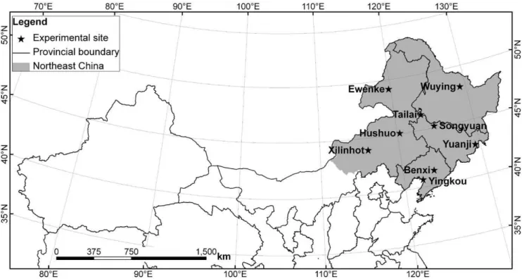
Northeast China consists of Heilongjiang, Jilin, Liaoning provinces and four leagues of Inner Mongolia (Fig. 1). The region has a continental monsoon climate. Mean annual air temperature is 4.5uC, with an average temperature of218.2uC in the coldest month (January), and an average of 22.4uC in the warmest month (July). Annual average precipitation is 514 mm, 77% of which falls from May to August. The region has a minimum annual precipitation of 245 mm in the west, a typical semi-arid area, and a maximum annual precipitation of 1079 mm in the east.
In the east of Northeast China, Great Xing’an Mountains is the cold temperate coniferous forest zone, dominated by typical tree species Larix dahurica. Changbai mountains, typical temperate coniferous and broadleaved mixed forest zone, dominated byPinus koraiensis. The west of Northeast China is the typical zone of temperate steppe with herbs such asLeymus chinensis,Stipa krylovii, Agropyron cristatum and S. baicalensis [20]. In Northeast China, Populus simonii is the main afforestation tree species, and Salix matsudana, Armeniaca vulgaris, and Ulmus pumila are the common garden species. These plant species are strictly controlled by hydrothermal conditions. Thus, thirteen dominant plant species are selected in the present study, including eight trees (Salix matsudana, Armeniaca vulgaris, Ulmus pumila, Populus simonii, Syringa oblate, Pinus koraiensis, Larix dahurica, and Picea koraiensis) and five
herbs (Leymus chinensis, Stipa krylovii, S. baicalensis, Elymus dahuricus, andAgropyron cristatum) (Table 1).
Phenological data collection
The leafing data of dominant plants were collected from nine Agricultural Meteorological Experiment Stations, China Meteo-rological Administration, located in Northeast China. Plant leafing status was observed daily; plants were considered to have leafed if: (1) the first flat leaf had appeared from the buds of trees with simple leaves; (2) young leaves had emerged from the leaf sheaths of conifers; (3) one or two leaflets of compound leaves had unfolded; or (4) old exposed leaves of over-wintering herbs had turned from yellow to green, and the first leaf of herbs had emerged above the ground [21].
Meteorological data collection
Meteorological data, including daily mean temperature, daily precipitation, daily minimum temperature and relative humidity, were collected from nine Agriculture Meteorological Stations where plant leafing was observed.
Phenology model
Generally, temperature is considered to be the main driving factor of plant leafing. Representative temperature-based phenol-ogy models include spring warming model (SW) [14], sequential model (SM) [9,10,22], parallel model (PM) [9,10,23], and alternating model (AM) [8,10,23]. These four models were used to simulate leafing in the present study. Their equations are summarized in Table 2 [23].
Water plays a critical role in regulating plant phenology in arid and semi-arid areas [18,24,25], and has been included in some phenology models. Examples include cumulative precipitation in the current year [26], vapor pressure deficit in the growth season index (GSI) [25], and soil moisture [18]. However, the
Figure 1. Locations of the study area and nine Agricultural Meteorological Experiment Stations in Northeast China. doi:10.1371/journal.pone.0033192.g001
A Temperature-Precipitation Based Leafing Model
combination of hydrological and thermal factors has not been considered. Usually, when both hydrological and thermal conditions reach certain thresholds, plants begin leafing. Previous studies of plant leafing phenology [18,24] have identified the accumulated precipitation in the previous year and current year as an important hydrological factor and the accumulated tempera-ture in the current year as an important thermal factor affecting plant leafing. Thus, a new plant leafing model (so-called TP) based on the effects of both temperature and precipitation could be expressed as:
Pcrit~k1|Pbzk2|
X
y
1
Riand F~
X
y
1
(Ti{Tb) Ti§Tbð1Þ
where k1, k2, Pcrit, Tb, and F *
are parameters obtained through optimization. k1, k2 are the efficiency of precipitation in the previous and current (prior to leafing) year in affecting leafing in the current year. Pb is the annual precipitation in the previous year.yis the day of plant leafing in the current year.Riis the daily precipitation in the current year (mm).Pcritis the water threshold (mm).Tiis the average daily temperature (uC) in the current year. Tbis the base temperature (uC).F*is the temperature sum critical threshold (uC). Models should always be validated with indepen-dent data not used to construct the model itself [27]. In this study, the phenology model parameters were estimated using leafing data from odd-numbered years (12 years), and the simulation accuracy was tested with the independent even-year data (12 years).
Parameter estimation
Phenological data were converted to Julian day (DOY). Model parameters were estimated using the least root mean square error (RMSE) method:
RMSE~
ffiffiffiffiffiffiffiffiffiffiffiffiffiffiffiffiffiffiffiffiffiffiffiffiffiffiffiffiffiffiffiffiffiffiffi Pn
i~1
(di(x){diobs)2
n
v u u u t
ð2Þ
wheredi(x) is the predicted date of plant leafing in theith year and diobs is the observed value of plant leafing in the ith year. The model was evaluated byF-tests. The optimized parameters of the model were determined using the simulated annealing method [8].
The averageRMSE, coefficient of determination (R2) were used to validate the model in the present study.
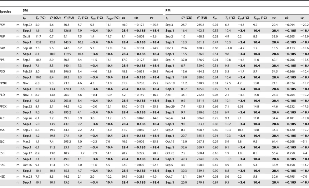
Using odd-year data, the parameter sets and three statistic variables (RMSE,R2and F) were given in Tables 3, 4, 5 for five models (i.e., SW, SM, PM, AM, and TP) (Table 2). Both fixed and parameterized starting date were considered for SW, TP and AM, i.e., the fixed starting date was set on 1 January for SW and TP and 1 September for AM. The starting date (t0), the minimum
(Tlow) and maximum (Thigh) values of chill temperature, and the
parameters values (va, vb, vc) of response curves for forcing temperature were fixed (e.g.,t0,Tlow,Thigh,va,vbandvcwere set to
September 1,23.4, 10.4, 28.4,20.185 and218.4, respectively) and parameterized for SM and PM, based on the reference and parameterization in the present study.
Results Model fitting
The model comparison would be evaluated by RMSE, coefficients of determination (R2) and sum of residual squares (e.g.,F-test). The averageRMSEfor all models fitting ranged from 2.00 to 4.18. The average RMSEs of PM with all parameters estimated (PMm) was the smallest, and the averageRMSEs of SM with all parameters estimated (SMm) was close behind (Tables 3, 4, 5). However, the result of models fitting did not represent an accurate model test. The model validation would be assessed using independent data.
The averageRMSEs of temperature - precipitation based leafing model (TP) with fixed and parameterized starting date were 3.22 and 2.69 days, respectively.k1(average = 0.05) of TP was smaller thank2(average = 0.45) (Table 3). The hydrological conditions for plant leafing varied with available water and climate in different regions. Thus, model coefficients comprehensively reflected the hydrological requirements for plant leafing. The mean hydrolog-ical requirement for woody plants was more than herbs in Northeast China.
Model validation
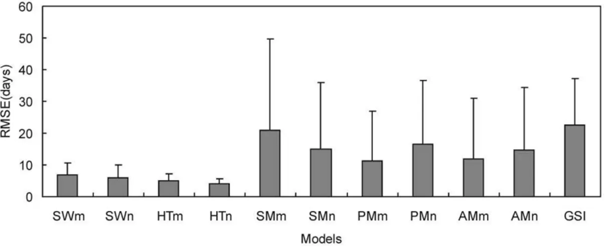
We validated these models using plant leafing data of even-numbered years in Northeast China. TP with fixed starting date (TPn) had the smallest averageRMSE(4.21 days). TheRMSEsof TPn for all plant species ranged from 2.22 to 6.44 days. The averageRMSEof TP with parameterized starting date (TPm) was 5.12 days. The average RMSE of SW with fixed starting date Table 1.Observation sites in Northeast China and the plant species studied for leafing at those sites.
Location Province Longitude (6E) Latitude (6N) Elevation (m) Species
Observation period (year)
Benxi Liaoning 123.78 41.32 182.5 Salix matsudana 1981–2005
Yingkou Liaoning 122.27 40.67 4.3 Syringa oblate 1981–2005
Songyuan Jilin 124.83 45.18 139.7 Populus simonii 1981–2005
Yuanji Jilin 129.40 42.77 240.6 Armeniaca vulgaris 1984–2005
Tailai Heilongjiang 123.42 46.40 149.5 Ulmus pumila 1982–2004
Wuying Heilongjiang 129.25 48.12 299.1 Pinus koraiensis Larix dahurica Picea koraiensis
1991–2002 1991–2002 1991–2002
Xilinhot Inner Mongolia 116.07 43.95 991 Leymus chinensis Stipa krylovii 1985–2004 1985–2004
Ewenke Inner Mongolia 119.75 49.15 621 Leymus chinensis Stipa baicalensis 1986–2006 1986–2006
Hushuo Inner Mongolia 120.33 45.07 629 Elymus dahuricus Agropyron cristatum
1980–2006 1988–2006
(SWn) was smaller than SW with parameterized starting date (SWm) (i.e., 6.09 days ,6.95 days). The averageRMSEs of the other models were more than 10 days (Fig. 2, Fig. 3).
For tree leafing, R2 was greater than 0.60 for 75% of the estimates by SWn and TPn, but less than 50% for the others. Both SWn and TPn had RMSEless than five days in 87.5% of the
estimates, while they met this criterion less than 75% of the time (Table 6). Based onR2
andRMSE, SWn and TPn were the best models for simulating tree leafing in Northeast China.
When we validated the models using even-year data for herb leafing, TPn model yieldedRMSEof 4–6 days (average 5.03 days) andR2of 0.4–0.82 (average 0.675); followed by TPm with average Table 2.Equations of the phenology models compared in the present study.
Model type Equation of models
Spring warming model (SW)
Sf~P y
t0
Rf(xt)~F
Rf(xt)~
0 xtƒTb
xt{Tb xtwTb
Sequential model (SM)
Sf~P y
t1
Rf(xt)~F
Rf(xt)~ 0 xt
ƒTb
va=(1zevb|(xtzvc)) x
twTb
C~P
t1
t0
Rc(xt)
Rc(xt)~
0
(xt{Tlow)=(To{Tlow)
(xt{Thigh)=(To{Thigh) 8
<
:
xtƒTlow xt§Thigh
TlowvxtvTo
TovxtvThigh
Parallel model (PM)
Sf~P y
t0
Rf(xt)~F
Rf(xt)~
0
(Kmz(1{Km)|Sc=C)|f(xt)
f(xt) 8 <
:
xtƒ0 and ScvC xtw0 and ScvC
xtw0 and Sc§C
f(xt)~va=(1zevb|(xtzvc))
Sc~P y
t0
Rc(xt)
Rc(xt)~ 0
(xt{Tlow)=(To{Tlow)
(xt{Thigh)=(To{Thigh) 8
<
:
xtƒTlow xt§Thigh
TlowvxtvTo
TovxtvThigh
Alternating model (AM)
Sf~P y
t1
Rf(xt)~F~a|eb|Sc
C~P
t1
t0
Rc(xt)
Sc~P y
t0
Rc(xt)
Rc(xt)~
0 1
xtwTb
xtƒTb
Rf(xt)~ 0x t{Tb
xtƒTb
xtwTb
Growth season index (GSI)
iTmin~ 0 (Tminz2)=7 1
8 <
:
Tminƒ{2 {2vTminv5
Tminw5
iVPD~
0
1{(VPD{900)=3200 1
8 <
:
VPD§4100pa 900pavVPDv4100pa
VPDƒ900pa
iPhoto~ 0
(Photo{36000)=3000 1
8 <
:
Photoƒ36000s 36000svPhotov39600s
Photo§39600s
iGSI~iTmin|iVPD|iPhoto
y: date of leafing;xt: daily mean air temperature in degrees Celsius;Rf(xt): forcing rate function;Rc(xt): chilling rate function;Sf: state of forcing;Sc: state of chilling;Km:
minimum potential of unchilled buds to respond to forcing temperature;C*: critical value of state of chilling for the transition from rest to quiescence;F*: temperature sum critical threshold;t0: starting day of the heat sum calculation or date of onset of rest;t1: date of onset of quiescence;Tb: base temperature;To: optimal temperature
of the rate of chilling;Tlow: the lowest temperature of the rate of chilling;Thigh: the highest temperature of the rate of chilling;a,b,va,vbandvc: constants;iTmin: daily
indicator for minimum temperature;Tmin: observed daily minimum temperature in degrees Celsius;iVPD: daily indicator for vapor pressure deficit;VPD: observed daily
vapor pressure deficit in Pascals;iPhoto: daily photoperiod indicator;Photo: daily photoperiod in seconds;iGSI: daily growing season index. doi:10.1371/journal.pone.0033192.t002
A Temperature-Precipitation Based Leafing Model
RMSEandR2
of 6.21 days and 0.572, respectively. For the other models, the minimum and average RMSEwere more than 4.50 and 9.51 days, respectively (Fig. 2), and the maximum and average R2 were less than 0.62 and 0.22, respectively (Table 6). Consequently, TPn was the best model for simulating herb leafing in the present study.
Discussion
Previous works have suggested thatR2[28] orRMSE[29] are
better than other criteria for comparing different nonlinear models. Generally, the smaller the RMSEvalue, the larger theR2value. However, the opposite case (i.e., a smallerRMSEwas associated with a smallerR2) occasionally appeared in the model calibration of SW and TP for leafing of Salix matsudana(Table 5). SWn could simulate the leafing ofSalix matsudanaprecisely (R2= 0.67,P,0.001) (Table 6). This result supports the opinion that RMSEis a more
reliable measure of fit thanR2
for nonlinear regression [29]. The opposite case may be due to the noise of parameterized data forS. matsudana. Furthermore, the RMSEof plant leafing in Northeast China given by TPn ranged from 2.22 to 6.44 days, and the predicted DOY values for leafing were close to the observed values (Fig. 4). It indicated that TP can precisely simulate the leafing stages of both woody plants and herbs in Northeast China.
The model accuracy for tree leafing at high latitudes could not necessarily be improved with more complex models, consistent with the result of Hannerz [30]. In the present study, the most complicated model, PM, could give better simulation with the least precise, while a much simpler model, SW, with more accurate. SM, AM, and PM consider all the factors in the chilling process, whereas SW and TP do not, i.e., the former models include more information on temperature change through time during param-eterization process. However, these three models (SM, AM, and Table 3.Parameter values of spring warming model (SW), temperature-precipitation based leafing model (TP), and alternating model (AM) for plant leafing in Northeast China.
Species SW TP AM
t0 Tb(6C) F*(6C day) t0 Tb(6C) F*(6C day) k1 k2 Pcrit(mm) t0 Tb(6C) C*(CU) a b
PSM m Apr.12 0.6 36.8 Apr. 12 7.4 6.2 0.044 0.669 28.49 Nov. 8 0.1 2.13 215.2 20.0431
n Jan. 1 0.2 209.0 Jan. 1 6.2 53.3 0.013 0.040 20.34 Sep. 1 0.0 28.47 835.2 0.05
PUP m Apr.10 1.3 199.2 Apr 11 2.8 150.6 0.018 0.216 9.63 Oct. 7 8.8 1.32 52.03 20.0385
n Jan. 1 0.9 271.6 Jan. 1 0.2 284.1 0.044 0.650 9.12 Sep. 1 7.2 2.13 85.37 20.02
PAV m Mar.30 7.0 69.4 Mar. 20 7.0 68.7 0.099 0.579 21.48 Sep. 14 7.6 3.39 53.06 20.0013
n Jan. 1 7.0 68.6 Jan. 1 3.0 176.5 0.054 0.088 31.64 Sep. 1 7.3 3.30 55.90 20.03
PPS m Mar.22 0.0 280.6 Mar. 30 0.1 247.9 0.088 0.450 26.29 Oct. 4 0.5 11.52 353.5 20.0269
n Jan. 1 3.3 178.3 Jan. 1 5.7 110.7 0.095 0.800 16.75 Sep. 1 0.0 5.23 299.0 20.01
PSO m Apr.1 9.1 25.7 Apr. 11 9.0 26.1 0.015 0.849 4.92 Feb. 24 7.5 9.74 62.2 20.0241
n Jan. 1 0.0 288.6 Jan. 1 2.1 210.2 0.096 0.993 21.38 Sep. 1 9.0 9.16 46.5 20.01
PPNK m May29 0.0 554.2 Jun. 8 2.4 325.4 0.012 0.120 23.18 Sep. 3 14.6 0.21 107.8 20.0323
n Jan. 1 1.2 903.3 Jan. 1 9.3 293.6 0.010 0.179 34.04 Sep. 1 14.6 0.93 115.1 0.08
PLD m May1 4.7 123.1 May 1 5.4 107.0 0.034 0.403 16.58 Sep. 8 4.3 0.52 200.7 20.0812
n Jan. 1 3.1 217.3 Jan. 1 9.8 38.69 0.023 0.447 13.33 Sep. 1 5.7 1.77 151.2 20.04
PPCK m May 11 9.2 67.7 Apr. 28 1.0 325.3 0.023 0.295 13.67 Sep. 25 7.4 0.28 135.6 20.0462
n Jan. 1 2.1 352.1 Jan. 1 0.5 468.0 0.049 0.073 22.66 Sep. 1 7.4 4.65 161.6 20.04
XLC m Apr.16 2.3 16.1 Mar. 19 2.2 45.4 0.076 0.158 15.48 Mar. 26 2.4 4.76 52.17 20.0683
n Jan. 1 1.1 83.9 Jan. 1 2.3 44.3 0.073 0.168 15.18 Sep. 1 1.6 2.45 99.28 20.09
XSK m Apr.11 3.3 6.0 Mar. 20 0.5 52.6 0.079 0.094 14.84 Oct. 4 0.0 0.64 109.3 20.0818
n Jan. 1 4.1 19.7 Jan. 1 0.1 58.4 0.097 0.104 18.09 Sep. 1 1.6 1.85 53.25 20.01
ELC m Apr.10 0.2 82.9 Jan. 17 0.0 108.1 0.052 0.166 12.61 Oct. 17 0.3 5.06 146.9 20.0951
n Jan. 1 0.5 98.5 Jan. 1 0.1 101.3 0.040 0.699 15.76 Sep. 1 4.6 21.33 58.0 20.01
ESB m Apr.11 0.4 84.0 Mar. 17 0.0 115.2 0.097 0.154 18.03 Oct. 5 0.8 0.42 102.4 20.0831
n Jan. 1 0.0 109.4 Jan. 1 0.1 114.3 0.024 0.771 8.63 Sep. 1 0.1 30.6 168.0 20.02
HAC m Apr.9 7.3 12.4 Mar. 25 1.5 67.5 0.035 0.702 14.89 Mar. 23 7.1 12.43 28.8 20.071
n Jan. 1 1.5 92.3 Jan. 1 1.5 64.7 0.036 0.847 16.00 Sep. 1 5.6 14.13 40.6 20.04
HED m Apr.12 3.0 45.2 Apr. 9 6.7 7.9 0.046 0.937 19.54 Mar.11 1.6 10.54 96.2 20.0174
n Jan. 1 1.1 101.1 Jan. 1 0.3 89.7 0.042 0.446 15.86 Sep.1 6.2 8.64 46.3 20.08
m: parameterized starting date (t0); n: fixed starting date (t0);Tb: base temperature;F*: temperature sum critical threshold;k1: efficiency of precipitation in the previous
Table 4.Parameter values of sequential model (SM) and parallel model (PM) for plant leafing in Northeast China.
Species SM PM
t0 Tb(6C) C*(CU) F*(FU) To(
6C) Tlow(6C) Thigh(6C) va vb vc t0 C*(CU) F*(FU) Km To(
6C) Tlow(6C) Thigh(6C) va vb vc
PSM m Sep.22 5.9 5.6 50.3 5.7 5.5 11.1 40.0 20.172 225.8 Sep.3 28.7 265.8 0.05 6.2 24.3 9.2 29.4 20.094 220.2
n Sep.1 1.6 9.3 126.8 7.9 23.4 10.4 28.4 20.185 218.4 Sep.1 16.4 402.5 0.52 10.4 23.4 10.4 28.4 20.185 218.4
PUP m Oct.8 11.7 0.7 9.1 7.5 1.4 11.7 1.1 20.803 25.6 Sep.2 1.0 468.2 0.28 4.9 0.2 8.5 33.0 20.205 215.9
n Sep.1 12.8 12.8 143.5 10.2 23.4 10.4 28.4 20.185 218.4 Sep.1 13.3 361.2 0.47 10.3 23.4 10.4 28.4 20.185 218.4
PAV m Sep.28 7.5 9.6 24.6 6.2 5.3 12.9 6.4 20.101 224.9 Dec.1 20.6 100.5 0.60 24.0 24.2 1.2 15.5 20.113 218.6
n Sep.1 6.1 10.0 119.5 10.4 23.4 10.4 28.4 20.185 218.4 Sep.1 15.5 376.0 0.54 9.8 23.4 10.4 28.4 20.185 218.4
PPS m Sep.8 10.2 8.9 30.8 8.4 21.5 14.1 17.0 20.127 228.6 Sep.14 37.0 376.9 0.01 10.8 24.4 11.0 60.1 20.206 217.5
n Sep.1 7.1 8.3 140.1 7.3 23.4 10.4 28.4 20.185 218.4 Sep.1 8.7 329.0 0.31 9.8 23.4 10.4 28.4 20.185 218.4
PSO m Feb.25 3.0 18.5 396.3 1.4 24.6 13.8 48.8 20.051 220.5 Feb.4 15.6 484.2 0.13 5.5 21.7 5.7 54.5 20.366 210.4
n Sep.1 10.0 8.4 88.3 9.3 23.4 10.4 28.4 20.185 218.4 Sep.1 19.0 388.6 0.34 10.4 23.4 10.4 28.4 20.185 218.4
PPNK m Nov. 6.8 9.3 23.3 4.6 4.3 11.0 31.9 20.738 225.2 Feb.19 11.2 570.9 0.01 12.5 4.2 13.0 21.1 20.024 215.7
n Sep.1 21.0 13.4 120.3 22.6 23.4 10.4 28.4 20.185 218.4 Sep.1 83.7 405.0 0.19 5.3 23.4 10.4 28.4 20.185 218.4
PLD m Nov.13 8.7 13.8 26.0 6.6 20.4 10.9 6.2 20.159 216.2 Apr.1 34.1 222.8 0.06 2.1 24.8 15.0 23.3 20.264 210.2
n Sep.1 0.5 12.2 203.8 8.4 23.4 10.4 28.4 20.185 218.4 Sep.1 0.9 381.4 0.58 10.1 23.4 10.4 28.4 20.185 218.4
PPCK m Sep.22 8.1 2.1 44.2 4.2 22.0 12.1 15.0 20.178 225.8 Sep.29 7.4 423.3 0.66 7.1 6.08 14.8 44.6 20.232 217.3
n Sep.1 9.0 4.6 195.2 4.1 23.4 10.4 28.4 20.185 218.4 Sep.1 9.7 390.6 0.55 6.9 23.4 10.4 28.4 20.185 218.4
XLC m Sep.26 6.1 7.2 39.5 5.9 3.6 11.2 9.5 20.040 214.6 Sep.6 3.4 306.8 0.25 9.3 9.1 11.0 34.4 20.181 215.8
n Sep.1 5.0 13.9 43.8 9.2 23.4 10.4 28.4 20.185 218.4 Sep.1 9.0 373.3 0.86 10.2 23.4 10.4 28.4 20.185 218.4
XSK m Sep.21 6.3 19.5 44.3 2.2 2.1 14.0 41.9 20.069 222.7 Sep.2 0.2 408.7 0.60 10.3 10.3 10.8 34.3 20.120 219.7
n Sep.1 1.2 19.8 27.4 4.0 23.4 10.4 28.4 20.185 218.4 Sep.1 20.7 385.4 0.91 10.3 23.4 10.4 28.4 20.185 218.4
ELC m Mar.3 1.1 7.4 295.2 1.0 22.3 7.0 40.6 20.002 235.8 Oct.19 13.0 267.3 0.29 5.9 5.8 9.5 64.4 20.208 25.1
n Sep.1 6.1 11.2 23.1 0.7 23.4 10.4 28.4 20.185 218.4 Sep.1 32.6 260.7 0.96 9.1 23.4 10.4 28.4 20.185 218.4
ESB m Sep.17 0.9 13.0 18.9 21.7 22.9 14.1 20.9 20.229 220.5 Oct.20 7.5 560.4 0.16 1.9 1.8 8.5 56.4 20.250 24.4
n Sep.1 2.1 11.1 49.0 1.1 23.4 10.4 28.4 20.185 218.4 Sep.1 49.3 274.8 0.99 23.1 23.4 10.4 28.4 20.185 218.4
HAC m Oct.16 9.1 11.4 57.0 3.0 21.6 5.5 52.0 20.005 252.7 Sep.5 4.0 358.6 0.45 4.9 4.4 5.4 33.9 20.158 214.7
n Sep.1 10.1 10.4 15.3 4.7 23.4 10.4 28.4 20.185 218.4 Sep.1 30.3 339.4 0.90 8.8 23.4 10.4 28.4 20.185 218.4
HED m Mar.23 7.7 8.3 44.2 2.1 2.0 10.2 59.9 20.285 29.0 Oct.7 13.1 236.7 0.08 5.6 0.2 5.8 30.6 20.795 27.0
n Sep.1 10.1 10.1 15.6 4.4 23.4 10.4 28.4 20.185 218.4 Sep.1 20.0 370.1 0.99 9.5 23.4 10.4 28.4 20.185 218.4
m: all parameters estimated; n: section parameters estimated;Tlow: the lowest temperature of the rate of chilling; CU: chilling unit; FU: forcing unit;Thigh: the highest temperature of the rate of chilling;va,vbandvc: constants;Tb: base temperature;C*: critical value of state of chilling for the transition from rest to quiescence;F*: temperature sum critical threshold;T
o: optimal temperature of the rate of chilling;Km: minimum potential of unchilled buds to respond to forcing temperature. PSM =Salix matsudana; PUP =Ulmus pumila; PAV =Armeniaca vulgaris; PPS =Populus simonii; PSO =Syringa oblate; PPNK =Pinus koraiensis; PLD =Larix dahurica; PPCK =Picea koraiensis; XLC =Leymus chinensisin Xilinhot; XSK =Stipa krylovii; ELC =Leymus chinensisin Ewenki; ESB =Stipa baicalensis; HAC =Agropyron cristatum; HED =Elymus dahuricus. The fixed parameters from Chuine et al. (1998) are in bold. doi:10.1371/journal.pone.0033192.t004
A
Temperatur
e-Precipitatio
n
Based
Leafing
Model
PLoS
ONE
|
www.plos
one.org
6
April
2012
|
Volume
7
|
Issue
4
|
PM) performed poorly when validated using actual observed data at different times, as seen withUlmus pumila(Table 6).
SW and TP without chilling requirement considering the starting date can reflect the effect of temperature beyond base temperature at different periods on plant leafing. Models with both fixed starting date (SWn and TPn) on 1 January and parameter-ized starting day (SWm and TPm) were analyzed in the present study. We found that after the validation by independent data, SWn (average RMSE of 6.05 days) could give better leafing simulation than SWm (average RMSE of 6.95 days), and TPn (averageRMSEof 3.59 days) was better than TPm (averageRMSE of 4.31 days). This result indicated that the temperature beyond base temperature at most periods could affect plant leafing. Generally, the models with parameterized starting date can consider only the temperature beyond base temperature after
starting date, but the temperature before starting date might have important effect on plant leafing. In Northeast China, the coldest month is January with mean air temperature of 218.2uC. Compared with SWm and TPm, SWn and TPn can give better simulation in Northeast China because the effective temperature during longer period can be considered. According to the observation data, tree leafing tended to advance with the extent of 0.23 days yr21
during 1980–2005, and was significantly negatively correlated with temperature in February, March and April. Furthermore, the effect of average temperature in April and February on plant leafing was the largest (2.35 daysuC21) and the smallest (1.18 daysuC21), respectively [31]. Therefore, regarding to climate warming, the main driving factor of plant leafing should be temperature instead of light [32], and SWn and TPn could give better simulation of plant leafing.
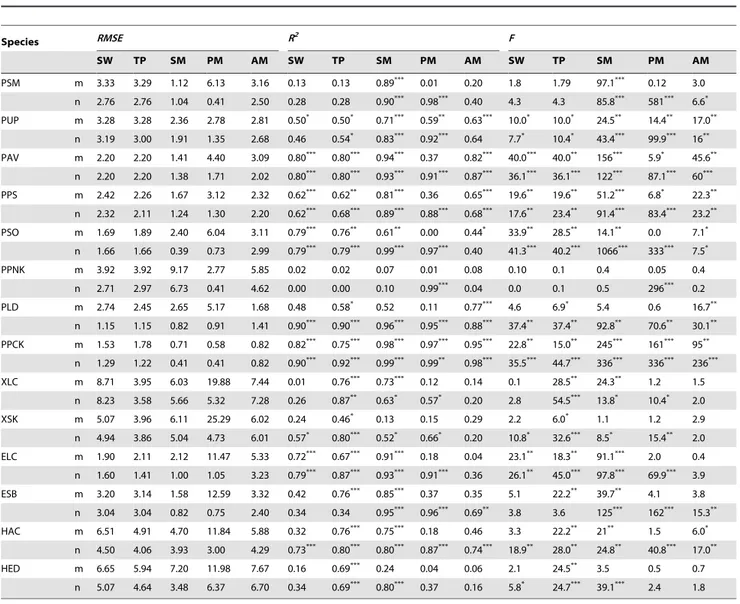
Table 5.Root mean square error (RMSE), coefficient of determination (R2) andF-test (F) for the model fitting to the data.
Species RMSE R2 F
SW TP SM PM AM SW TP SM PM AM SW TP SM PM AM
PSM m 3.33 3.29 1.12 6.13 3.16 0.13 0.13 0.89*** 0.01 0.20 1.8 1.79 97.1*** 0.12 3.0
n 2.76 2.76 1.04 0.41 2.50 0.28 0.28 0.90*** 0.98*** 0.40 4.3 4.3 85.8*** 581*** 6.6*
PUP m 3.28 3.28 2.36 2.78 2.81 0.50* 0.50* 0.71*** 0.59** 0.63*** 10.0* 10.0* 24.5** 14.4** 17.0**
n 3.19 3.00 1.91 1.35 2.68 0.46 0.54* 0.83*** 0.92*** 0.64 7.7* 10.4* 43.4*** 99.9*** 16**
PAV m 2.20 2.20 1.41 4.40 3.09 0.80*** 0.80*** 0.94*** 0.37 0.82*** 40.0*** 40.0** 156*** 5.9* 45.6**
n 2.20 2.20 1.38 1.71 2.02 0.80*** 0.80*** 0.93*** 0.91*** 0.87*** 36.1*** 36.1*** 122*** 87.1*** 60***
PPS m 2.42 2.26 1.67 3.12 2.32 0.62*** 0.62** 0.81*** 0.36 0.65*** 19.6** 19.6** 51.2*** 6.8* 22.3**
n 2.32 2.11 1.24 1.30 2.20 0.62*** 0.68*** 0.89*** 0.88*** 0.68*** 17.6** 23.4** 91.4*** 83.4*** 23.2**
PSO m 1.69 1.89 2.40 6.04 3.11 0.79*** 0.76** 0.61** 0.00 0.44* 33.9** 28.5** 14.1** 0.0 7.1*
n 1.66 1.66 0.39 0.73 2.99 0.79*** 0.79*** 0.99*** 0.97*** 0.40 41.3*** 40.2*** 1066*** 333*** 7.5*
PPNK m 3.92 3.92 9.17 2.77 5.85 0.02 0.02 0.07 0.01 0.08 0.10 0.1 0.4 0.05 0.4
n 2.71 2.97 6.73 0.41 4.62 0.00 0.00 0.10 0.99*** 0.04 0.0 0.1 0.5 296*** 0.2
PLD m 2.74 2.45 2.65 5.17 1.68 0.48 0.58* 0.52 0.11 0.77*** 4.6 6.9* 5.4 0.6 16.7**
n 1.15 1.15 0.82 0.91 1.41 0.90*** 0.90*** 0.96*** 0.95*** 0.88*** 37.4** 37.4** 92.8** 70.6** 30.1**
PPCK m 1.53 1.78 0.71 0.58 0.82 0.82*** 0.75*** 0.98*** 0.97*** 0.95*** 22.8** 15.0** 245*** 161*** 95**
n 1.29 1.22 0.41 0.41 0.82 0.90*** 0.92*** 0.99*** 0.99** 0.98*** 35.5*** 44.7*** 336*** 336*** 236***
XLC m 8.71 3.95 6.03 19.88 7.44 0.01 0.76*** 0.73*** 0.12 0.14 0.1 28.5** 24.3** 1.2 1.5
n 8.23 3.58 5.66 5.32 7.28 0.26 0.87** 0.63* 0.57* 0.20 2.8 54.5*** 13.8* 10.4* 2.0
XSK m 5.07 3.96 6.11 25.29 6.02 0.24 0.46* 0.13 0.15 0.29 2.2 6.0* 1.1 1.2 2.9
n 4.94 3.86 5.04 4.73 6.01 0.57* 0.80*** 0.52* 0.66* 0.20 10.8* 32.6*** 8.5* 15.4** 2.0
ELC m 1.90 2.11 2.12 11.47 5.33 0.72*** 0.67*** 0.91*** 0.18 0.04 23.1** 18.3** 91.1*** 2.0 0.4
n 1.60 1.41 1.00 1.05 3.23 0.79*** 0.87*** 0.93*** 0.91*** 0.36 26.1** 45.0*** 97.8*** 69.9*** 3.9
ESB m 3.20 3.14 1.58 12.59 3.32 0.42 0.76*** 0.85*** 0.37 0.35 5.1 22.2** 39.7** 4.1 3.8
n 3.04 3.04 0.82 0.75 2.40 0.34 0.34 0.95*** 0.96*** 0.69** 3.8 3.6 125*** 162*** 15.3**
HAC m 6.51 4.91 4.70 11.84 5.88 0.32 0.76*** 0.75*** 0.18 0.46 3.3 22.2** 21** 1.5 6.0*
n 4.50 4.06 3.93 3.00 4.29 0.73*** 0.80*** 0.80*** 0.87*** 0.74*** 18.9** 28.0** 24.8** 40.8*** 17.0**
HED m 6.65 5.94 7.20 11.98 7.67 0.16 0.69*** 0.24 0.04 0.06 2.1 24.5** 3.5 0.5 0.7
n 5.07 4.64 3.48 6.37 6.70 0.34 0.69*** 0.80*** 0.37 0.16 5.8* 24.7*** 39.1*** 2.4 1.8
SW: Spring warming model; TP: Temperature-precipitation based leafing model; AM: Alternating model; SM: Sequential model; PM: Parallel model. m: parameterized starting date for SW, TP and AM, all parameters estimated for SM and PM; n: fixed starting date for SW, TP and AM, section parameters estimated for SM and PM. PSM =Salix matsudana; PUP =Ulmus pumila; PAV =Armeniaca vulgaris; PPS =Populus simonii; PSO =Syringa oblate; PPNK =Pinus koraiensis; PLD =Larix dahurica; PPCK =Picea koraiensis; XLC =Leymus chinensisin Xilinhot; XSK =Stipa krylovii; ELC =Leymus chinensisin Ewenki; ESB =Stipa baicalensis; HAC =Agropyron cristatum; HED =Elymus dahuricus.
*:P,0.05; **:P,0.01; ***:P,0.001.
The simulation precision of phenology models with the consideration of chilling is critically influenced by the starting date. In Europe, phenology models are set to start on 1 September [23] or 1 November [7,10]. In this study, SMn, PMn and AMn were set to start on 1 September and the starting dates of SMm, PMm and AMm were parameterized using odd-year data. There are largerRMSEsfor those models from independent data, and the reasons are attributed to the starting date: (1) the starting date is set
early, resulting in untimely meeting the chilling and forcing thermal requirements. For example, theRMSEof SM with starting date on 1 September and 16 October forAgropyron cristatumwere 58.9 and 11.57 days, respectively (Table 4, Fig. 3); and (2) the starting date is set late, leading that chilling thermal requirement can not meet. e.g., the RMSE of SM with starting date on 1 September was smaller (3.87 days) than 13 November (92.33 days) forLarix dahurica(Table 3, Fig. 3).
Figure 2. The root mean square error (RMSE) of different phenology models for plant leafing using independent data.Tree species include PSM =Salix matsudana; PUP =Ulmus pumila; PAV =Armeniaca vulgaris; PPS =Populus simonii; PSO =Syringa oblate; PPNK =Pinus koraiensis; PLD =Larix dahurica; and PPCK =Picea koraiensis. Herbs include XLC =Leymus chinensisin Xilinhot; XSK =Stipa krylovii; HED =Elymus dahuricus; HAC =Agropyron cristatum; ELC =Leymus chinensis in Ewenki; and ESB =Stipa baicalensis. SWn, TPn, and AMn: Spring warming model (SW), Temperature-precipitation based leafing model (TP), and Alternating model (AM) with fixed starting date. SWm, TPm, and AMm: SW, TP and AM with parameterized starting date. SMn and PMn: Sequential model (SM) and Parallel model (PM) with section parameters estimated. SMm and PMm: SM and PM with all parameters estimated. GSI: Growth season index.
doi:10.1371/journal.pone.0033192.g002
Figure 3. Average root mean square error (RMSE) of different phenology models for plant leafing using independent data.SWn, TPn, and AMn: Spring warming model (SW), Temperature-precipitation based leafing model (TP), and Alternating model (AM) with fixed starting date. SWm, TPm, and AMm: SW, TP and AM with parameterized starting date. SMn and PMn: Sequential model (SM) and Parallel model (PM) with section parameters estimated. SMm and PMm: SM and PM with all parameters estimated. GSI: Growth season index.
doi:10.1371/journal.pone.0033192.g003
A Temperature-Precipitation Based Leafing Model
The fixed parameters (t0,Tlow,Thigh, va, vband vc) in SM and PM, from the result of Europe [9,11,12,16], were widely used in plant phenology models [10,21,23]. Furthermore, these parame-ters were estimated using local observing data [31]. In the model fitting process of the present study, all thresholds and parameters of SM and PM were estimated. We found that the models with many parameters could be fitted well (Tables 3, 4, 5), but could not give accurate simulation when tested with the independent data (Fig. 2). This finding was consistent with the result from Linkosalo et al. [33], and it might be because the models were over-parameterized and able to adapt to noise in addition to the
phenological phenomenon itself [33]. The parameter estimate lies on the parameter space boundary [34].
Variation in the base temperature has no significant effect on the precision of spring phenology models [14,30,35]. Generally, the heat unit total depends on the threshold used [35], as with Leymus chinensisin this study (Tables 3, 4, 5). Therefore, changes in the base temperature induce different thresholds for the accumu-lated temperature, resulting in no significant variation in model accuracy. The threshold measure is a mathematical construct which may or may not be related to the physiological threshold [34]. Physiological parameters can be estimated from simulation experiments, but can not be obtained from the process of parameter optimization. This is because the optimization process is mostly dependent on the precision of observed field data, sample number, and local climate conditions. The biological interpreta-tion of model parameters should not be considered as absolute [34,36]. The base leafing temperature of the same plant can be different simply due to different models, as seen with all plant species in this study (Tables 3, 4, 5). The base temperature in the growth season index (GSI) is fixed, and the minimum temperature is derived from experimental data [36,37]. In the present study, the leafing dates of woody plants actually changed can be, to a certain extent, explained by GSI using the fixed parameter. However, considering the threshold of 0.5 from the original model [25], the predicted dates for plant leafing in Northeast China was earlier than the observed values. Thus, the original parameter threshold for GSI was too small for the present study, and the optimal threshold varied with different species.
Previous studies indicated that the phenology of woody plants in temperate regions can be accurately predicted by a temperature-based model (e.g., SW). For example, SW is considered to be the best model to accurately simulate the bud development ofPicea abies [30] and has been validated [23]. Chilling has been introduced into some temperature-based models (e.g., AM) to improve accuracy. For example, AM is much more suitable for simulating budburst of Picea abies [7]. Furthermore, there is a correlation between chilling and forcing, i.e., forcing takes the effect after the chilling has finished [38].
In this study, plant leafing in Northeast China was simulated using four temperature-based and two temperature-precipitation based phenology models. When validated with independent data, SW and TP could give best simulation of the woody plant leafing. The effect of temperature in TP was the same with SW, and its accuracy was consistent with SW in moist conditions. The effect of precipitation in TP does not change the model manner of temperature, therefore (1) TP with fixed starting date (TPn) could be used to simulate the leafing affected by hydrological factors. For example, leafing ofLeymus chinensis and Stipa kryloviiin Xilinhot, Inner Mongolia was delayed 27 and 22 days due to water stress in some years; in other locations, the average delay time forLeymus chinensis, Stipa baicalensis, Elymus dahuricus and Agropyron cristatum reached 7, 5, 14 and 16 days, respectively; and (2) the leafing of woody plants in Northeast China was mainly driven by thermal conditions, and hydrological conditions were not limiting factors. For example, the averageRMSEof SWn was much close to TPn for tree leafing (Fig. 2). This finding was consistent with other studies in which the precision simulating the leafing of broad-leaved deciduous plants could not be substantially improved by adding precipitation into the model [26]. Kramer et al. [39] also believed that, in temperate zone, water availability mainly affects leaf area index and has little effect on leaf phenology. However, different species have different sensitivities to water conditions, and the leafing of some trees may be affected by hydrological conditions. Thus, TP is suitable for a wider range of plants Table 6.Coefficient of determination (R2) of model
verification using independent data for the plant leafing in Northeast China.
Species SW TP SM PM AM GSI
PSM m 0.53** 0.56** 0.69*** 0.76*** 0.58** 0.47*
n 0.67*** 0.66*** 0.72*** 0.72*** 0.67***
PUP m 0.58** 0.66*** 0.31 0.30 0.23 0.59**
n 0.82*** 0.80*** 0.28 0.26 0.28
PAV m 0.65*** 0.64*** 0.73*** 0.69*** 0.69*** 0.61**
n 0.64*** 0.65*** 0.66*** 0.57** 0.77***
PPS m 0.74*** 0.80*** 0.52** 0.56** 0.57** 0.46*
n 0.74*** 0.72*** 0.79*** 0.24 0.53
PSO m 0.23 0.22 0.37 0.76*** 0.64*** 0.79***
n 0.84*** 0.82*** 0.46* 0.58** 0.45*
PPNK m 0.05 0.13 0.01 0.31 0.20 0.72**
n 0.45 0.42 0.00 0.01 0.35
PLD m 0.92*** 0.92*** 0.00 0.60* 0.70** 0.94***
n 0.96*** 0.97*** 0.96*** 0.58* 0.48
PPCK m 0.14 0.48 0.14 0.21 0.22 0.24
n 0.34 0.24 0.33 0.29 0.15
XLC m 0.04 0.80*** 0.06 0.17 0.11 0.00
n 0.02 0.82*** 0.00 0.37 0.10
XSK m 0.11 0.68** 0.03 0.08 0.00 0.00
n 0.33 0.69** 0.06 0.45* 0.21
ELC m 0.09 0.58* 0.62** 0.52* 0.32 0.06
n 0.02 0.40* 0.23 0.17 0.02
ESB m 0.22 0.50* 0.47* 0.37 0.46* 0.18
n 0.51* 0.53* 0.54* 0.09 0.51*
HAC m 0.02 0.69** 0.01 0.18 0.00 0.48*
n 0.03 0.80*** 0.01 0.13 0.00
HED m 0.01 0.18 0.08 0.01 0.07 0.04
n 0.00 0.81*** 0.01 0.09 0.05
SW: Spring warming model; TP: Temperature-precipitation based leafing model; SM: Sequential model; PM: Parallel model; AM: Alternating model; GSI: Growth season index. m: parameterized starting date for SW, TP and AM, all parameters estimated for SM and PM; n: fixed starting date for SW, TP and AM, section parameters estimated for SM and PM. PSM =Salix matsudana; PUP =Ulmus pumila; PAV =Armeniaca vulgaris; PPS =Populus simonii; PSO =Syringa oblate; PPNK =Pinus koraiensis; PLD =Larix dahurica; PPCK =Picea koraiensis; XLC =Leymus chinensisin Xilinhot; XSK =Stipa krylovii; ELC =Leymus chinensisin Ewenki; ESB =Stipa baicalensis; HAC =Agropyron cristatum; HED =Elymus dahuricus.
*:P,0.05; **:P,0.01; ***:P,0.001.
because it considers the effects of both temperature and precipitation on plant leafing.
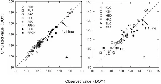
TP was far superior to other five models in estimating herb leafing in Northeast China, and all simulated dates were very close to the observed dates (Fig. 4B). Other five models can not accurately simulate herb leafing. In addition to temperature, water availability was shown to be an important controlling factor for the phenology of herbs [18]. For example, the annual precipitation of 5 years (1984, 1989, 2000, 2001, and 2002) was less than 210 mm in Xilinhot, and was negatively correlated with herb leafing in next year (R2
.0.9; Fig. 5). Therefore, the reduction of previous annual
precipitation leads to the delay of herb leafing. It is reasonable to consider the effect of previous annual precipitation in TP. Because herbs generally have shallow roots, they tend to be strongly affected by hydrological conditions. Herb leafing in response to environmental conditions can be estimated using hydrological factors incorporated into the TP model. Although GSI can model the effects of hydrological factors with vapor pressure deficit (VPD), the validation of the model was rather poor in the present study, due to the lack of available VPD value or the lower sensitivity of VPD to hydrological conditions (Fig. 4). In addition, two instances can indicate that TP is superior over SW in more Figure 4. Observed versus simulated values for tree (A) and herb (B) leafing in Northeast China based on Temperature-precipitation based leafing model (TPn). Tree species include PSM =Salix matsudana; PUP =Ulmus pumila; PAV =Armeniaca vulgaris; PPS =Populus simonii; PSO =Syringa oblate; PPNK =Pinus koraiensis; PLD =Larix dahurica; and PPCK =Picea koraiensis. Herbs include XLC =Leymus chinensis in Xilinhot; XSK =Stipa krylovii; HED =Elymus dahuricus; HAC =Agropyron cristatum; ELC =Leymus chinensisin Ewenki; and ESB =Stipa baicalensis.
doi:10.1371/journal.pone.0033192.g004
Figure 5. Relationship between annual precipitation in previous year and leafing of two herbs (i.e.,Leymus chinensisandStipa krylovii) in Xilinhot, Inner Mongolia.
doi:10.1371/journal.pone.0033192.g005
A Temperature-Precipitation Based Leafing Model
arid areas: (1) theRMSEof TPn was smaller than that of SWn for Leymus chinensis and Stipa krylovii in arid Xilinhot, and (2) the predicted leafings from SWn and TPn with the sameTband F* were very close in moist years, and much closer to the observed value from TPn in drought years than SWn (data not shown).
Phenology model parameters can be obtained experimentally, but most phenology models use parameters optimized based on long-term observed data, e.g., the four temperature-based models (SW, SM, PM, and AM) and the temperature-precipitation based leafing model (TP). Different parameters are selected for different plant species in various regions. Therefore, sufficient data should be used to ensure the effectiveness and reliability of the model parameters. In this study, leafing simulations ofPinus koraiensisand Picea koraiensiswere poor because the parameters were optimized based on only six years’ observed data (Table 6, Fig. 2). There is a strong possibility that more errors occur when the model is based
on less data. However, the parameters of leafing phenology models for the other six woody plants were optimized using 12 years’ observed data, and all models accurately simulated plant leafing. Overall, TP will be more suitable and reliable for modeling both woody and herbaceous plant leafing given climate changes (especially variation in hydrological conditions), while other leafing models that do not consider water will be less applicable in semi-arid and semi-arid areas.
Author Contributions
Conceived and designed the experiments: GZ RL. Performed the experiments: RL. Analyzed the data: RL. Contributed reagents/materi-als/analysis tools: GZ RL. Wrote the paper: RL. Contributed to the revision of the manuscript: GZ.
References
1. Goulden ML, Munger JW, Fan SM, Daube BC, Wofsy SC (1996) Exchange of carbon dioxide by a deciduous forest: response to interannual climate variability. Science 271: 1576–1578.
2. White MA, Running SW, Thornton PE (1999) The impact of growing-season length variability on carbon assimilation and evapotranspiration over 88 years in the eastern US deciduous forest. Int J Biometeorol 42: 139–145.
3. Hogg HE, Price DT, Black TA (2000) Postulated feedbacks of deciduous forest phenology on seasonal climate patterns in the western Canadian interior. J Climate 13: 4229–4243.
4. Molod A, Salmun H, Waugh DW (2003) A new look at modeling surface heterogeneity: Extending its influence in the vertical. J Hydrometeorol 4: 810–825.
5. Running SW, Hunt ER (1993) Generalization of a forest ecosystem process model for other biomes, BIOME-BGC, and an application for global-scale models. In: Field C, Ehleringer J, eds. Physiological processes, leaf to glob, Academic Press, New York. pp 141–158.
6. Schwartz MD (1998) Green-wave phenology. Nature 394: 839–840. 7. Cannell MGR, Smith RI (1983) Thermal time, chill days and prediction of
budburst inPicea sitchensis. J Appl Ecol 20: 951–963.
8. Chuine I (2000) A unified model for budburst of trees. J Theor Biol 207: 337–347.
9. Ha¨nninen H (1990) Modelling bud dormancy release in trees from cool and temperate regions. Acta Forestalia Fenn 213: 1–47.
10. Kramer K (1994) Selecting a model to predict the onset of growth ofFagus sylvatica. J Appl Ecol 31: 172–181.
11. Richardson EA, Seeley SD, Walker DR (1974) A model for estimating the completion of rest for ‘Redhaven’ and ‘Elberta’ peach trees. Hort Science 9: 331–332.
12. Sarvas R (1972) Investigations on the annual cycle of development of forest trees. Active Period Commun Instituti Forestalis Fenn 76: 1–110.
13. Diekmann M (1996) Relationship between phenology of perennial herbs and meteorological data in deciduous forests of Sweden. Can J Bot 74: 528–537. 14. Hunter AF, Lechowicz MJ (1992) Predicting the timing of budburst in temperate
trees. J Appl Ecol 29: 597–604.
15. Ha¨nninen H (1987) Effects of temperature on dormancy release in woody plants: Implications of prevailing models. Silva Fenn 21: 279–299.
16. Landsberg JJ (1974) Apple fruit bud development and growth; analysis and an empirical model. Ann Bot 38: 1013–1023.
17. Murray MB, Cannell MGR, Smith RI (1989) Date of budburst of fifteen tree species in Britain following climatic warming. J Appl Ecol 26: 693–700. 18. Yuan WP, Zhou GS, Wang YH (2007) Simulating phenological characteristics
of two dominant herb species in a semi-arid steppe ecosystem. Ecol Res 22: 784–791.
19. Deng ZY, Wang Q, Zhang Q, Qing JZ, Yang QG, et al. (2010) Impact of climate warming and drying on food crops in northern China and the countermeasures. Acta Ecol Sin 30: 6278–6288. (in Chinese with English abstract).
20. Guo ZX, Zhang XN, Wang ZM, Fang WH (2010) Responses of vegetation phenology in Northeast China to climate change. Chinese J Ecol 29: 578–585. (in Chinese with English abstract).
21. China Meteorological Administration (1993) Norms of Agricultural Meteoro-logical Observation. MeteoroMeteoro-logical Press, ISBN: 7-5029-1383-1/P.0600. 22. Chuine I, Cambon G, Comtois P (2000) Scaling phenology from the local to the
regional level: advances from species-specific phenological models. Global Change Biol 6: 943–952.
23. Chuine I, Cour P, Rousseau DD (1998) Fitting models predicting dates of flowering of temperate-zone trees using simulated annealing. Plant Cell Environ 21: 455–466.
24. Chen XQ, Li J (2009) Relationships betweenLeymus chinensisphenology and meteorological factors in Inner Mongolia herblands. Acta Ecol Sin 29: 5280–5290. (in Chinese with English abstract).
25. Jolly WM, Nemani R, Running SW (2005) A generalized, bioclimatic index to predict foliar phenology in response to climate. Global Change Biol 11: 619–632.
26. White MA, Thornton PE, Running SW (1997) A continental phenology model for monitoring vegetation responses to interannual climatic variability. Global Biogeochem Cy 11: 217–234.
27. Chatfield C (1988) Problem solving: a statistician guide. Chapman and Hall, London.
28. Logan JA (1988) Toward an expert system for development of pest simulation models. Environ Entomol 17: 359–376.
29. Draper NK, Smith H (1981) Applied regression analysis. 2nd
ed. Wilde, New York.
30. Hannerz M (1999) Evaluation of temperature models for predicting bud burst in Norway spruce. Can J Forest Res 29: 9–19.
31. Li RP, Zhou GS (2010) Response of woody plants phenology to air temperature in Northeast China in 1980–2005. Chinese J Ecol 29: 2317–2326. (in Chinese with English abstract).
32. Linkosalo T, Lechowicz MJ (2006) Twilight far-red treatment advances leaf bud-burst of silver birch (Betula pendula). Tree Physiol 26: 1249–1256.
33. Linkosalo T, Lappalainen HK, Hari P (2008) A comparison of phenological models of leaf bud burst and flowering of boreal trees using independent observations. Tree Physiol 28: 1873–1882.
34. Ma ZS, Bechinski EJ (2008) Developmental and phenological modeling of Russian wheat aphid (Hemiptera: Aphididae). Ann Entomol Soc Am 101: 351–361.
35. Thomson AJ, Moncrieff SM (1982) Prediction of bud burst in Douglas-fir by degree-day accumulation. Can J For Res 12: 449–452.
36. Larcher W, Bauer H (1981) Ecological significance of resistance to low temperature. In: Lange OL, Nobel PS, Osmond CB, Zeigler H, eds. Encyclopedia of plant physiology, new series, Springer-Verlag, Berlin. pp 403–437.
37. Zimmerman MH (1964) Effect of low temperature on ascent of sap in trees. Plant Physiol 39: 568–572.
38. Ha¨nninen H, Pelkonen P (1989) Dormancy release inPinus sylvestrisL. andPicea abies(L.) Karst. seedlings: Effects of intermittent warm periods during chilling. Trees-Struct Funct 3: 179–184.