Ashwini M. Deshpande
1and Suprava Patnaik
21
Department of Electronics and Telecommunication Engineering, TSSM’s Bhivarabai Sawant College of Engineering and Research, Narhe
Pune (MS), India
2Department of Electronics Engineering, S. V. National Institute of Technology, Surat
ABSTRACT
Considering the sparseness property of images, a sparse representation based iterative deblurring method is presented for single image deblurring under uniform and non-uniform motion blur. The approach taken is based on sparse and redundant representations over adaptively training dictionaries from single blurred-noisy image itself. Further, the K-SVD algorithm is used to obtain a dictionary that describes the image contents effectively. Comprehensive experimental evaluation demonstrate that the proposed framework integrating the sparseness property of images, adaptive dictionary training and iterative deblurring scheme together significantly improves the deblurring performance and is comparable with the state-of-the art deblurring algorithms and seeks a powerful solution to an ill-conditioned inverse problem.
KEYWORDS
Image Deblurring, Non-Uniform Blur, Sparse Representation, Adaptive Dictionary
1. INTRODUCTION
Single image deblurring is one of the most active research areas in the field of image processing. Being an inherently ill-posed problem, seeking a solution in terms of correct pair of an unknown degradation function and original image from the blurred and noisy observation, is quite challenging as there can be multiple combinations of these two unknowns that might have resulted into the available blurred-noisy image.
A high-quality image undergoes blurring, be it due to atmospheric blur (in astronomy), defocusing, camera shake blur (in photography), or any other possible source. Typically, motion blur is caused when there is a relative motion between the camera and the object being imaged during an exposure time. Even in case of lack of ambient light, slower shutter speed is necessary to increase exposure time, where camera shake is likely to happen and degrades the image quality significantly. Complex motion paths as in the case of camera shake are particularly challenging as blur kernels are arbitrary and any kind of parametric model to represent the same is infeasible.
repository in removal of uniform and non-uniform motion blur from a single blurred-noisy image. Comparative performance analysis performed with some of the leading deblurring algorithms proves the effectiveness of the proposed method in handling blurs like linear blur, camera shake, hand shake etc.
Although the degradation process, in general, is nonlinear and space varying, a large number of problems could be addressed with a sophisticated linear and shift-invariant (LSI) model. Hence the observation process in the imaging system, with an assumption of blur to be translation invariant and pixel-location independent can be modelled as,
g x y( , )= f x y( , )⊗h x y( , )+n x y( , ) (1)
where ⊗ is a 2-D convolution operator, function f represents an unknown original image, h is PSF of the image formation system, g is the observed blurred-noisy image and n denotes additive noise. This convolutional model can approximate many real world blurring processes very well, and also provides simplified computational form in the frequency domain. Thus, the task of single image deblurring is to restore a sharp image from a single blurred and noisy observation.
The image formulation process can also be modelled in matrix-vector form or in frequency domain. Defining g, h, f, and n as the vector versions of g(x, y), h(x, y), f(x, y) and n(x, y), respectively, the matrix-vector formulation is,
g=Hf +n (2)
where H is a two-dimensional sparse matrix with elements taken from h(x, y) to have the proper mapping from f to g, equivalently, the Fourier-domain description of the imaging model is,
G u v( , )=H u v F u v( , ) ( , )+N u v( , ) (3)
where G(u, v), F(u, v), H(u, v) and N(u, v) are the Fourier transforms of g(x, y), f(x, y), h(x, y) and n(x, y) respectively. In general, frequency domain analysis of an imaging system provides additional cues about the behavior of the imaging system. In our work, while referring to the sparse representation of the observed blurred-noisy image, a matrix-vector form is used and, for the sake of convenience, frequency domain model is used for iterative image deblurring part.
The rest of the paper is organized as: in Section 2, a brief review of recent advances in image deblurring techniques is presented. Problem formulation, sparse model for image deblurring and dictionary learning process are covered in Section 3. Section 4 discusses an iterative image deblurring approach taken up in the proposed algorithm whereas a complete proposed single image deblurring technique- SparseD is put forth in Section 5. Experimental set-up as well as subjective and objective results compared with state-of-the art methods are presented in Section 6 and conclusions are provided in Section 7.
2. RELATED WORK
If the PSF is unknown then the problem is termed as blind deconvolution or blinddeblurring. Early work on blind deblurring usually consider a single image and assume a prior parametric form of the blur kernel so that the blur kernel can be obtained by only estimating a few parameters. Linear motion blur kernel model used in these works often is too simplified, whereas for true motion blurring in practice blur kernel is often an arbitrary form. To solve more complex motion blurring, either a pair of images [6] or multi-image based approaches have been proposed to obtain more information of the blur kernel by either actively or passively capturing multiple images on the scene [7, 8].
Recently, a progressive development has been initiated for removing complex motion blurs from a single image. There are two typical approaches of algorithms that can be categorized as Bayesian (probabilistic) and regularization. The class of Bayesian framework based algorithms use some probabilistic priors either on latent image or on blur kernels or images’ edge distribution, to derive the blur kernel [9, 10, 11] or manually selecting blurred edges to obtain the local blur kernel [12]. Possible limitation on this type of method is that, the assumed probabilistic priors may not always hold true for general or natural images. The other popular approach is to formulate the blind deconvolution problem as a joint minimization problem with the consideration of some regularization constraints on both the blur kernel and the latent image. Among the existing regularization-based methods, TV (Total Variation) norm and its variations have been the dominant choice of the regularization term to solve various blind deblurring problems [13]. Shan et al. [14] presented a more sophisticated minimization model where the fidelity term is a weighted l2 norm on the similarity of both image intensity and image gradients.
Sparse representation recently has attracted community of researchers in the field of image processing for solving problems such as deblurring, denoising, super resolution etc. Sparsity principle is used for approximating signals as a linear combination of a few dictionary elements. The property of sparsity in the representation of signals has also been approved in human perception by some studies of human vision. Olshausen et al. [15] represented a natural image using a small number of basis functions [16]. The sparse representation problem is usually solved through l0 (generally intractable) and l1 (tractable) minimization with non-negativity constraints.
The progress of l0-norm and l1-norm minimization techniques have been successfully applied to
many vision tasks, including face recognition [17], image super resolution [16, 18] etc. Also, with the growing realization that regular separable 1−D wavelets are inappropriate for handling images, several new tailored multi-scale and directional redundant transforms are introduced, including the curvelet, contourlet, wedgelet, bandlet and the steerable wavelet [19, 20] etc. to design suitable dictionaries.
In [21], the authors introduced the K-SVD algorithm, a way to learn a dictionary, rather than using a predefined dictionary [22]. In parallel, the introduction of the matching pursuit [23] and the basis pursuit denoising [24] gave rise to the ability to address the image denoising problem as a direct sparse decomposition technique over redundant dictionaries. Begovic et al. [25] provide an extension and upgradation of the K-SVD dictionary learning concept from non-scalable to scalable adaptive image reconstruction by regularizing the learning process of dictionary elements.
results presented in our proposed method are superior over the method in [29]. Instead of image deblurring, blurred image classification based on adaptive dictionary is reported in [30].
Above mentioned methods either utilized prior statistics learned from or assumed for a single, a pair or a set of additional images for deblurring [9, 31, 14], whereas our proposed algorithm requires only a single input image.
Under the framework of sparse representation, the proposed method takes advantage of dictionary learning in adaptive fashion from the observed blurred-noisy image and inclusion of iterative deblurring approach.
3. SPARSE REPRESENTATION FOR IMAGE DEBLURRING
It is well-known that natural images can be modelled with sparse representation over an over-complete dictionary. A signal (input image) can be approximated by a sparse linear combination of atom signals in an over-complete dictionary. This Section introduces problem formulation and terminologies used in sparse modeling for image deblurring problem.
3.1. Problem Formulation
To construct a sparse model of an input image it is assumed that the original image f is of size
n× npixels, where n = 256. The input image degradation is due to a known linear
space-invariant blur kernel H and an additive zero-mean white Gaussian noise with known variance
σ
2. A blurred and noisy image g, is also of the same size as the input image which is formulated as g = Hf + n. Now to recover sharp image f is the desired goal, where it is also assumed that f can be very well described as D with a known dictionary D and a sparse vector [32]. It becomes a minimization problem which is described as follows:Consider the linear system,
f∈R fn =D
α
(4)where, D∈Rn m× is the overcomplete dictionary and is the decomposition coefficient of f. There are many solutions of f = D , and the least number of non-zero coefficients i could be found.
Therefore, the degradation model in Eq. (2) can be equivalently modelled as,
g = HD
α
+ n (5)To solve such l0-minimization problem Donoho [33] proposed the step as,
0
ˆ arg min s t. . g HD n
α
=α
=α
+ (6)where, 0
α
is l0-norm (i.e., the nonzero entries of ). The problem in Eq. (5) is computationallyNP-hard, however, referring to work of Donoho [33], to relax the non-convex sparsity problem to convex problem it can be revised as,
1
ˆ arg min s t. . g HD n
2
1 2
1 min
2 g HD
α
λ α
+ −α
(8) where the first item is called as the sparse penalty function and the second item is the data fidelity term.3.2. Dictionary Learning
The over-complete dictionary (i.e., a learned set of parameters) formation is an important step for sparse representation. For the image deblurring algorithm, we should specify the dictionary D, such that it could lead to an efficient sparse representation modeling of underlying image content. Instead of deploying any pre-chosen set of basis functions such as the wavelet, steerable wavelet, curvelet or contourlet, in the proposed deblurring algorithm, learning the dictionary adaptively from the corrupted (blurred and noisy) image is the way chosen.
3.2.1. Dictionary Learning Process
Basically, K-SVD is a direct extension of a well-known K-means clustering method and it is used for dictionary learning purpose in our work. K-means method encodes each sample using a single clustering center, while K-SVD method sparsely encodes the samples using atoms from the dictionary D. The K-SVD [21] dictionary learning process is an iterative method of training a dictionary from a set of images or image patches. The goal of K-SVD is to find the overcomplete dictionary D which is a sparse representation for the training signals. The K-SVD algorithm is used to construct the overcomplete dictionary, flexible with pursuit algorithm (Matching pursuit (MP), Basic pursuit (BP)). The model of K-SVD could be described as follows:
2 0
2 0
,
min . . i,
Dα G−D
α
s t ∀α
<T (9) where, T0 is given sparsity level,{ }
1n
i
g = g = are the training signals, is the relevant coefficient
and D is the dictionary to be found. There are two stages in K-SVD algorithm:
• Sparse Coding Stage: Using MP or BP and
• Dictionary Update Stage: update one atom at a time.
The sparse coding is performed for each signal individually using any standard technique. A dictionary update step in K-SVD, performed atom-by-atom is more easier and efficient process over a matrix inversion task. An example of trained dictionary obtained during the experimentation of proposed method, for uniform and non-uniform motion blurred house image (with
σ
=0.5 andσ
=1.5 ) is shown in Figure 1.
(a) (b)
3.2.2. Pursuit algorithms and OMP
The problem in Eq. (5) is computationally NP-hard and there are two main approaches to approximate the solution to such problem: The first approach is the greedy family of methods, where an attempt is to build the solution one non-zero at a time. The second approach is the relaxation methods, which attempt to solve the problem by smoothing the l0-norm and using
continuous optimization techniques [32]. All these techniques aim to approximate the solution of the problem posed in Eq. 5 and are commonly referred to as pursuit algorithms. The most basic algorithm is the matching pursuit (MP). This is an iterative algorithm that starts by finding one atom that best describes the input signal.
In [34], the authors proposed a refinement of the MP algorithm which improves convergence using an additional orthogonalization step. The orthogonal matching pursuit (OMP) is an improvement of the MP. The OMP re-computes the set of coefficients for the entire support each time an atom is added to the support. This stage speeds up the convergence rate, as well as ensures that once an atom has been added to the support, it will not be selected again. This is a result of the least-squares stage, making the residual orthogonal to all atoms in the chosen support. For a finite dictionary with N elements, OMP is guaranteed to converge to the projection onto the span of the dictionary elements in a maximum of N steps. Due to all such advantages of OMP algorithm it is chosen as a relaxation method to obtain
α
ˆ.The restored image is thus obtained as,gˆ=D
α
ˆ, and goal of the experimentation is to get as close as possible to the original image in terms mean squared error minimization.4.
I
MAGER
ESTORATION:
A
NI
TERATIVED
EBLURRINGA
PPROACHThere are number of image restoration methods, such as, Wiener filter, Richardson-Lucy algorithm, constrained least-squares filtering, Bayesian and non-Bayesian methods etc.; a detail survey of these techniques is very well covered in [35].
Numbers of such algorithms impose spatial and Fourier domain constraints on the PSF and true image estimates, and update initial estimates iteratively. In [36], nonnegativity on both the PSF and true image is imposed by setting negative values to zero in spatial domain. In Fourier domain, the current estimate F(i) is updated as,
F(i+1)( , )u v (1
γ
)F( )i ( , )u vγ
G u v H( , ) ( )i ( , )u v= − + (10)
which is essentially a weighted average of F(i)(u, v) and G(u, v)/H(i)(u, v) with a weight parameter
γ
. The first part Fi is obtained by taking the Fourier transform of f(i) and therefore imposes the constraint of spatial-domain nonnegativity. Second part G(u, v)/H(i)(u, v) is a result of Fourier domain constraint G(u, v) =(H(i)(u, v) F(i)(u, v)). H(i)(u, v) is updated in the same way as in Eq. (10) by exchanging H(i)(u, v)and F(i)(u, v). In this algorithm there is no theoretical optimal value forγ
and needs to be found empirically. Another way to represent Eq. (10) is to express it in terms of Wiener-like update:( 1) 2 ( ) 2 ( ) ( , ) ( , ) ( , ) ( , ) ( , ) i i i
H u v G u v F u v
H u v
F u v
η
∗ + = + (11)In this paper, we have formulated a new iterative image deblurring approach by combining the Wiener-like [1] update approach with the conventional iterative blind deconvolution [36] approach. This formulation is given as:
( 1) ( ) 2
( )
( , ) ( , ) ( , ) ( , )
( , )
i i
i
H u v G u v F u v F u v
H u v
η
∗ +
= +
+
(12)
This iterative deblurring step tries to minimize frequency residual error and it is alternated with dictionary update stage which gives rise to a proposed sparse iterative deblurring algorithm -
SparseD, which is summarized in the next Section.
5. PROPOSED SPARSE ITERATIVE DEBLURRING ALGORITHM - SPARSED
With a combination of alternate step of dictionary updating for sparse representation of input observation and iterative image deblurring approach as described in Section 4, a new Sparse iterative deblurring algorithm is put forth with adaptive dictionary learning. The main steps performed in the algorithm are as follows:
1. Initialize the dictionary D from Discrete cosine transform (DCT) bases
2. Repeat following steps till mean squared error (MSE) gets minimized or there is further improvement in terms of peak signal-to-noise ratio (PSNR) for deblurred image
3. Initialize f0 =g0 (as initial estimate)
4. Update dictionary D from input blurred-noisy image using K-SVD algorithm
5. Perform iterative deblurring (set noise energy,
η
=0.35) with known PSF• Take Fourier transform of ith estimation f(i) i.e., F(i)(u, v)
• Compute F(i+1)(u, v) according to Eq. (12)
• Apply inverse Fourier transform on F(i+1)(u, v)
• Impose non-negativity constraint on above equation and obtain deblurred image
6. Using trained dictionary from step 4 and deblurred image from step 5, obtain
α
ˆ with the help of OMP algorithm7. Obtain restored image as: gˆ=D
α
ˆAlternating between iterative deblurring and denoising, by updating dictionary from recent output has lead proposed SparseD algorithm into satisfactory performance for removal of a complex motion blurs in presence of noise. Experimental evaluation proves the effectiveness of this algorithm.
6. EXPERIMENTAL EVALUATION
blur kernels are used to simulate motion blur in presence of varying amount of additive Gaussian noise as described below. The experimental setup used to simulate blurred images is as given as,
• Uniform motion blur kernel (Blur parameters: L=15pixels and
θ
=400)• 8 different Non-uniform blur kernels as given in [10]
• Additive Gaussian white noise with
σ
n =0.5andσ
n =1.5Quantitative comparison of proposed algorithm and competitive single image deblurring methods is carried on the basis of PSNR and Structural SIMilarity (SSIM) index as performance metrics.
(a)
(b)
Figure 2. Example of test images (a) house, boat and lena, (b) test images collected from [20]
Combination of one of the types of blur as listed above, along with an additive Gaussian white noise with different values of standard deviation,
σ
are added to simulate blurred-noisy images. The deblurring results by the proposed SparseD method are then compared with three state-of-the-art methods i.e., Wiener filter, Richardson-Lucy (RL) algorithm and deblurring algorithm of Shan et. al [14]. To verify the effectiveness and the robustness of proposed SparseD method, both quantitative (PSNR and SSIM measures) and qualitative results are presented. PSNR and SSIM results are reported in a tabular form followed by deblurring results as well. One can see in the visual comparison that there are many noise residuals and artifacts around edges in the deblurred images in the competing methods.6.1. Experiment 1: Uniform motion blur with noise
After simulating motion blur with the blur parameters blur length, L = 15 pixels and blur angle, 0
40
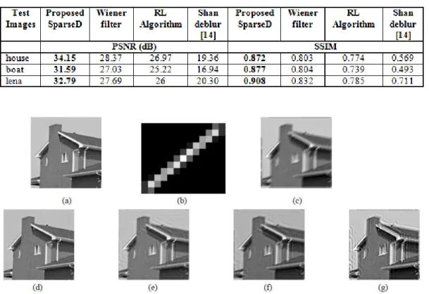
Table 1. PSNR (dB) and SSIM results of deblurred images (uniform motion blur with blur parameters 15
L= pixels and
θ
=400) (σ
n=0.5)Figure 3. Test image: house; case: uniform motion blur (L=15pixels and
θ
=400) (σ
n= 0.5) (a) Original image, (b) Motion blur kernel, (c) Noisy-blurred image, and Deblurred images by: (d) SparseDmethod, (e)Wiener filter, (f) R-L algorithm (g) Shan deblur [14]
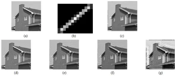
Figure 4. Test image: house; case: uniform motion blur (L = 15 pixels and
θ
=400) (σ
n= 1.5) (a) Original image, (b) Motion blur kernel, (c) Noisy-blurred image, and Deblurred images by: (d) SparseDmethod, (e)Wiener filter, (f) R-L algorithm (g) Shan deblur [14]
As shown in Figures 3 and 4 the visual appearance is pleasing in case of proposed method whereas some noise residuals and ringing artifacts around edges in the deblurred images are present in other cases. Even after changing the blur parameter values over a wide range of blur parameters and sigma values of noise from smaller to larger extent, proposed method maintains superiority over the competing methods.
6.2. Experiment 2: Non-uniform blur with noise
Most promising results are obtained in case of non-uniform blur removal with additive noise. This experiment is of particular interest as the non-uniform kernels portray camera shake effect, which is tedious to remove from single blurred image even after knowing (by some means either estimation or hardware attachment) the blur kernels. In this experiment, 8 different non-uniform blur kernels are collected from the dataset of Levin et al. [10] which are generated with actual camera setup. These kernels are shown in Figure 5.
Figure 5. Non-uniform blur kernels [10] and their sizes: (a) f1 (19 × 19), (b) f2 (17 × 17), (c) f3 (15 × 15), (d) f4 (27 × 27), (e) f5 (13 × 13), (f) f6 (21 × 21), (g) f7 (23 × 23), (h) f8 (23 × 23)
Table 3. SNR (dB) and SSIM results of deblurred images (Non-uniform blur kernel f4[10]) (
σ
n=0.5)Figure 6. Test image: boat; case: non-uniform blur kernel (kernel f4 [10])(
σ
n = 0.5) (a) Original image, (b) Non-uniform blur kernel, (c) Noisy-blurred image, and Deblurred images by: (d) SparseD method, (e)Wiener filter, (f) R-L algorithm (g) Shan deblur [14]Figure 7. Test image: boat; case: non-uniform blur kernel (kernel f4 [10])(
σ
n = 1.5) (a) Original image, (b) Non-uniform blur kernel, (c) Noisy-blurred image, and Deblurred images by: (d) SparseDmethod, (e)Wiener filter, (f) R-L algorithm (g) Shan deblur [14]
In the same experimental scenario, some more results are added for different non-uniform kernels with moderate to high noise, so as to verify the robustness of the proposed method. The results are shown in Figure 8.
Figure 8. (a) Original image, (b) Non-uniform blur kernel (f1 [10]), (c) Noisy-blurred image (moderate noise,
σ
n= 25), (d) Deblurred using proposed SparseD method, (e)Non-uniform blur kernel (f2 [10]), (f) Noisy-blurred image (high noise,σ
n= 100), (g) Deblurred using proposed SparseD method7. CONCLUSIONS
effectively. The quality of the deblurred image inspected visually as well as quantitatively (PSNR and SSIM) shows that the proposed method performs far superior in comparison with two non-blind and one non-blind deblurring algorithm. It shows the usefulness of this method to deblur camera shaken images in practical applications such as photography, forensics, satellite and medical imaging fields. Proposed algorithm can be further enhanced in terms of fast optimization step.
ACKNOWLEDGEMENTS
The authors would like to thank anonymous reviewers for their constructive comments and valuable suggestions that helped to improve the quality of this work.
R
EFERENCES[1] N. Wiener, (1949) “Extrapolation, Interpolation and Smoothing of Stationary Time Series with Engineering Applications”, The MIT Press, Cambridge (Mass.), Wiley and Sons, New York.
[2] L. Lucy, (1974) “An iterative technique for the rectification of observed distributions,” The Astronomical Journal, vol. 79, no. 6, pp. 745–754.
[3] W. H. Richardson, (1972) “Bayesian-based iterative method of image restoration,” Journal of the Optical Society of America, vol. 62, no. 1, pp. 55–59.
[4] T. Chan and S. Esedoglu, (2005) “Aspects of total variation regularized ill function approximation,” in SIAM Journals, vol. 5, pp. 1817–1837.
[5] R. Neelamani, H. Choi, and R. Baraniuk, (2004) “Forward: Fourier-wavelet regularized deconvolution for ill-conditioned systems,” IEEE Transactions on Signal Processing, vol. 52, no. 2, pp. 418–433.
[6] L. Yuan, J. Sun, L. Quan, and H.-Y. Shum, (2007) “Image deblurring with blurred/noisy image pairs,” in SIGGRAPH ’07: ACM SIGGRAPH 2007, ACM, New York.
[7] M. Ben-Ezra and S. K. Nayar, (2004) “Motion-based motion deblurring,” IEEE Transactions on Pattern Analysis and Machine Intelligence, vol. 26, no. 6, pp. 689–698.
[8] R. Raskar, A. Agrawal, and J. Tumblin, (2006) “Coded exposure photography: motion deblurring using fluttered shutter,” ACM Trans. Graph., vol. 25, pp. 795–804.
[9] R. Fergus, B. Singh, A. Hertzmann, S. Roweis, and W. Freeman, (2006 ) “Removing camera shake from a single photograph,” ACM Transactions on Graphics(TOG), vol. 25, no. 3, pp. 787–794. [10] A. Levin, Y. Weiss, F. Durand, and W. Freeman, (2009) “Understanding and evaluating blind
deconvolution algorithms,” in Proceedings of the IEEE Conference on CVPR.
[11] N. Joshi, R. Szeliski, and D. Kriegman, (2008) “PSF estimation using sharp edge prediction,” in Proceedings of the IEEE Conference on Computer Vision and Pattern Recognition.
[12] J. Jia, (2007) “Single image motion deblurring using transparency,” IEEE Computer Society conference on computer vision and pattern recognition, pp. 1–8.
[13] T. F. Chan and C. K. Wong, (1998) “Total variation blind deconvolution,” in IEEE Trans. Image Process., vol. 7, no. 3, pp. 370–375.
[14] Q. Shan, J. Jia, and A. Agarwala, (2008) “High-quality motion deblurring from a single image,” in ACM Transactions on Graphics (SIGGRAPH), vol. 27, no. 3, pp. 73(1)–73(10).
[15] B. Olshausen and D. Field, (1997) “Sparse coding with an over-complete basis set: A strategy employed by v1,” in Vision Research, pp. 3311–3325.
[16] W. Dong, L. Zhang, G. Shi, and X. Wu, (2011) “Image deblurring and super-resolution by adaptive sparse domain selection and adaptive regularization,” in IEEE Trans. on Image Processing, pp. 1838– 1857.
[17] J. Wright, A. Yang, A. Ganesh, S. Sastry, and Y. Ma, (2009) “Robust face recognition via sparse representation,” in IEEE Trans. on Pattern Analysis and Machine Intelligence.
[18] J. Yang, J. Wright, T. Huang, and Y. Ma, (2008) “Image super resolution as sparse representation of raw patches,” in Proceedings of IEEE International Conference on CVPR.
[19] W. T. Freeman and E. H. Adelson, (1991) “The design and use of steerable filters,” in IEEE Pattern Anal. Mach. Intell., vol. 13, no. 9, pp. 891–906.
[20] M. N. Do and M. Vetterli, (2003) in Contourlets, Beyond Wavelets, E. N. Y. A. G. V. Welland, Ed.,. [21] M. Aharon, M. Elad, and A. Bruckstein, (2006) “K-SVD: An algorithm for designing of overcomplete
[22] J. Mairal, M. Elad, , and G. Sapiro, (2008) “Sparse representation for color image restoration,” in IEEE Trans. on Image Processing, vol. 17, no. 1, pp. 53–69.
[23] S. Mallat and Z. Zhang, (1993) “Matching pursuits with time-frequency dictionaries,” in IEEE Transaction on Signal Processing, vol. 12, pp. 3397–3415.
[24] S. S. Chen, D. L. Donoho, and M. A. Saunders, (2001) “Atomic decomposition by basis pursuit,” in SIAM Rev., vol. 43, no. 1, pp. 129–159.
[25] B. Begovic, V. Stankovic, and L. Stankovic, (2014) “Dictionary learning for scalable sparse image representation with applications,” in Advances in Signal Processing, vol. 2, no. 2, pp. 55 –74. [26] J.-F. Cai, H. Ji, C.-Q. Liu, and Z. Shen, (2009) “Blind motion deblurring from a single image using
sparse approximation,” in Computer Vision and Pattern Recognition, pp. 104 – 111.
[27] O. Whyte, J. Sivic, A. Zisserman, and J. Ponce, (2012) “Non-uniform deblurring for shaken images,” in IJCV. vol. 98, no. 2, pp. 168 – 186.
[28] H. Zhang, D.P. Wipf, and Y. Zhang, (2013) “Multi-image blind deblurring using a coupled adaptive sparse prior, ” in CVPR.
[29] H. Huang and N. Xiao, (2013) “Image deblurring based on sparse model with dictionary learning,” in Journal of Information and Computational Science, vol. 10, no. 1, pp. 129 – 137.
[30] G. Sun, J. Yin, and X. Zhou, (2013) “Blurred image classification based on adaptive dictionary,” in The International Journal of Multimedia & Its Applications (IJMA), vol.5, no.1, pp. 1–9.
[31] A. Levin, (2006) “Blind motion deblurring using image statistics,” In Advances in Neural Information Processing Systems (NIPS).
[32] M. Elad, (2010) Sparse and Redundant Representations: From Theory to Applications in Signal and Image Processing, Berlin: Springer.
[33] D. L. Donoho, (1995) “De-noising by soft-thresholding,” IEEE Transactions on Information Theory, vol. 41, no. 3, pp. 613–627.
[34] Y. C. Pati, R. Rezaiifar, and P. S. Krishnaprasad, (1993) “Orthogonal matching pursuit: Recursive function approximation with applications to wavelet decomposition,” in Proceedings of the Asilomar Conference on Signals, Systems, and Computers, vol. 1, pp. 40–44.
[35] D. Kundur and D. Hatzinakos, (1996) “Blind image deconvolution,” IEEE Signal Processing Mag., vol. 13, no. 3, pp. 43–64.
[36] G. R. Ayers and J. C. Dainty, (1988) “Iterative blind deconvolution method and its applications,” Optics Letters, vol. 13, no. 7, pp. 547–549.
[37] R. L. Lagendijk, J. Biemond, and D. E. Boekee, (1988) “Regularized iterative image restoration with ringing reduction,” in IEEE Transactions on Acoustics, Speech, and Signal Processing, vol. 36, no. 12, pp. 1874–1888.
AUTHORS
Ashwini M. Deshpande received the Bachelor’s Degree in Electronics Engineering from University of Pune and Master’s Degree from Shivaji University, Kolhapur. Presently she is a Research Scholar in the Department of Electronics Engineering, Sardar Vallabhbhai National Institute of Technology, Surat, (Gujarat) India. Her main research interests are in Signal Processing, Digital Image Processing and Analysis, Image Restoration, Signal Modelling etc.
![Figure 1. Example of trained dictionaries (size 64 × 256) for (a) Non-uniform blurred (kernel f 2 [20]) and noisy image, σ = 0.5 and (b) Uniform motion blurred and noisy image, σ = 1.5](https://thumb-eu.123doks.com/thumbv2/123dok_br/16438812.196587/5.918.255.677.825.991/figure-example-trained-dictionaries-uniform-blurred-uniform-blurred.webp)
![Figure 2. Example of test images (a) house, boat and lena, (b) test images collected from [20]](https://thumb-eu.123doks.com/thumbv2/123dok_br/16438812.196587/8.918.256.673.342.626/figure-example-test-images-house-boat-images-collected.webp)
![Table 3. SNR (dB) and SSIM results of deblurred images (Non-uniform blur kernel f 4 [10]) ( σ n = 0.5 )](https://thumb-eu.123doks.com/thumbv2/123dok_br/16438812.196587/11.918.167.768.161.568/table-snr-ssim-results-deblurred-images-uniform-kernel.webp)
![Figure 8. (a) Original image, (b) Non-uniform blur kernel (f 1 [10]), (c) Noisy-blurred image (moderate noise, σ n = 25), (d) Deblurred using proposed SparseD method, (e)Non-uniform blur kernel (f 2 [10]), (f) Noisy-blurred image](https://thumb-eu.123doks.com/thumbv2/123dok_br/16438812.196587/12.918.173.761.515.781/figure-original-blurred-moderate-deblurred-proposed-sparsed-uniform.webp)
