ISSN 2277-1956
/V1N3-1494-1503
Image Deblurring Using Sparse-Land Model
Harini. B 1, Dr. S.Nirmala 2
1- M.E VLSI Design, Muthayammal Engineering College
Rasipuram, Namakkal District, Tamilnadu, India, [email protected] 2- Head of the Department, Muthayammal Engineering College
Rasipuram, Namakkal District, Tamilnadu, India.
Abstract- In this paper, the problem of deblurring and poor image resolution is addressed and extended the task by removing blur and noise in the image to form a restored image as the output. Haar Wavelet transform based Wiener filtering is used in this algorithm. Soft Thresholding and Parallel Coordinate Descent (PCD) iterative shrinkage algorithm are used for removal of noise and deblurring. Sequential Subspace Optimization (SESOP) method or Line search method provides speed-up to this process. Sparse-land model is an emerging and powerful method to describe signals based on the sparsity and redundancy of their representations. Sparse coding is a key principle that underlies wavelet representation of images. Coefficient obtained after removal of noise and blur are not truly Sparse and so Minimum Mean Squared Error estimator (MMSE) estimates the Sparse vectors. Sparse representation of signals have drawn considerable interest in recent years. Sparse coding is a key principle that underlies wavelet representation of images. In this paper, we explain the effort of seeking a common wavelet sparse coding of images from same object category leads to an active basis model called Sparse-land model, where the images share the same set of selected wavelet elements, which forms a linear basis for restoring the blurred image.
Keywords : Parallel Coordinate Descent; Sparse representation; Minimum Mean Squared Error estimator; Sparse-land model
1. Introduction
Restoration of images has been the area of interest for researchers worldwide in the past two decades. Image restoration aims at deblurring the image. The main purpose is to compensate or undo some defects to restore the original image. Restoration has been achieved by various filtering techniques by estimating the degradation factor.
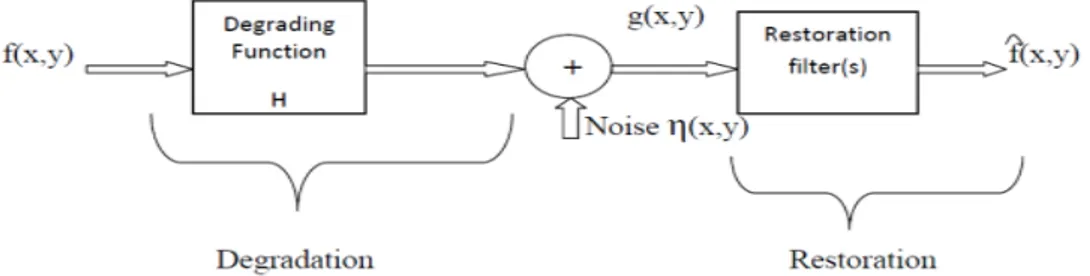
Fig. 1. Image Restoration Model
Figure 1 shows the restoration model. In the image restoration block the input function is f(x,y),which is being degraded by a function H. This forms the degradation block of the restoration model. The noise η(x,y) is added and the noisy image formed is represented by g(x,y). The restoration process can be achieved by designing suitable filters, with the knowledge of the degradation function. The efficiency of the restoration algorithm depends upon the degrading function. This restoration depends on the degrading function.
ISSN 2277-1956
/V1N3-1494-1503
The parameters of periodic noise typically estimated by inspection of the Fourier spectrum of the image. As noted in the, periodic noise tends to produce frequency spikes that often can be detected even by visual analysis. Another approach is to attempt to infer the periodicity of noise components directly from the image, but this is possible only in simplistic cases. Automated analysis is possible in situations in which the noise spikes are either exceptionally pronounced, or when some knowledge is available about the general location of the frequency components of the interference.
The parameters of noise PDF’s may be known partially from sensor specifications, but it is often necessary to estimate them for a particular imaging arrangement. If the imaging system is available, one simple way to study the characteristics of system noise is to capture a set of images of flat environment. For example, in the case of an optical sensor, this is as simple as imaging a solid gray board that is illuminated uniformly. The resulting images typically are good indicators of system noise.
The blurring, or degradation, of an image can be caused by many factors:
• Movement during the image capture process, by the camera or, when long exposure times are used, by the subject.
• Out-of-focus optics, use of a wide-angle lens, atmospheric turbulence, or a short exposure time, which reduces
the number of photons captured.
• Scattered light distortion in confocal microscopy.
2. Sparse Representation
In the last decade, sparsity has emerged as one of the leading concepts in a wide range of signal-processing applications (restoration, feature extraction, compression, to name only a few applications). Sparsity has long been an attractive theoretical and practical signal property in many areas of applied mathematics (such as computational harmonic analysis, statistical estimation, and theoretical signal processing).
In this paper, we explain the effort of seeking a common wavelet sparse coding of images from same object category leads to an active basis model called Sparse-land model, where the images share the same set of selected wavelet elements, which forms a linear basis for restoring the blurred image.
The aim of image restoration is the removal of noise (sensor noise, blur etc) from images. The simplest approach for noise removal is based on various types of filters such as low-pass filters or median filters. In this paper, we used Haar wavelet transform based Weiner filter followed by PCD algorithm. We observed that the outcomes does not show any tendency to be sparse. In this case, we start by defining a random generator of sparse vector and it can be modified in various ways. One among them is MMSE(Minimum mean square error) estimator and it is used in this paper. This analysis gives a more solid foundation for the sparsest representation of deblurred image, which is said to be Sparse-land model.
Recently, researchers spanning a wide range of viewpoints have advocated the use of overcomplete signal representations. Such representations differ from the more traditional representations because they offer a wider range of generating elements (called atoms).
2.1. Strictly Sparse Signals / Images
A signal x, considered as a vector in a finite-dimensional subspace of x = [x[1],…….x[N]], is strictly or exactly sparse if most of its entries are equal to zero, that is, if its support ∆(x) = {1 ≤ i ≤ N | x[i ] ≠0} is of cardinality k <<N. A k-sparse signal is a signal for which exactly k samples have a nonzero value. If a signal is not sparse, it may be sparsified in an appropriate transform domain. For instance, if x is a sine, it is clearly not sparse, but its Fourier transform is extremely sparse (actually, 1-sparse).
More generally, we can model a signal x as the linear combination of T elementary waveforms, also called signal atoms, such that
= = ∑ (1)
In approximation methods, typical norms used for measuring the deviation are the -norms for p=1,2,….. In this paper, we shall concentrate on the case p=2. If < and D is a full-rank matrix, an infinite number of solutions are available for the representation problem, hence constraints on the solution must be set. The solution with the fewest number of non zero coefficients is certainly an appealing representation. This sparsest representation is the solution of either
( ) ‖ ‖ subject to y=Dx (2) where ‖. ‖ is the norm, counting the nonzero entries of a vector.
ISSN 2277-1956
/V1N3-1494-1503
An overcomplete dictionary D that leads to sparse representations can either be chosen as a prespecified set of functions or designed by adapting its content to fit a given set of signal examples.Choosing a prespecified transform matrix is appealing because it is simpler. Also, in many cases it leads to simple and fast algorithms for the evaluation of the sparse representation. This is indeed the case for overcomplete wavelets, curvelets, contourlets, steerable wavelet filters, short-time Fourier transforms, and more. Preference is typically given to tight frames that can easily be pseudoinverted. The success of such dictionaries in applications depends on how suitable they are to sparsely describe the signals in question. Multiscale analysis with oriented basis functions and a shift-invariant property are guidelines in such constructions.
In this paper, we consider a different route for designing dictionaries D based on learning. Our goal is to find the dictionary D that yields sparse representations for the training signals. We believe that such dictionaries have the potential to outperform commonly used predetermined dictionaries.With evergrowing computational capabilities, computational cost may become secondary in importance to the improved performance achievable by methods that adapt dictionaries for special classes of signals.
3. Sparse Coding
Sparse coding is the process of computing the representation coefficients X based on the given signal Y and the dictionary D. This process, commonly referred to as “atom decomposition,” requires solving above equations, and this is typically done by a “pursuit algorithm” that finds an approximate solution. Exact determination of sparsest representations proves to be an NP-hard problem. Thus, approximate solutions are considered instead, and in the past decade or so several efficient pursuit algorithms have been proposed. The simplest ones are the matching pursuit (MP) and the orthogonal matching pursuit (OMP) algorithms. These are greedy algorithms that select the dictionary atoms sequentially. These methods are very simple, involving the computation of inner products between the signal and dictionary columns, and possibly deploying some least squares solvers. Both above equations are easily addressed by changing the stopping rule of the algorithm.
A second well-known pursuit approach is the basis pursuit (BP). It suggests a convexification of the problems posed in the above equations by replacing the -norm with an -norm. The focal underdetermined system solver (FOCUSS) is very similar, using the -norm with p≤ 1as a replacement for the –norm in the above equations. Here, for p< 1 the similarity to the true sparsity measure is better but the overall problem becomes nonconvex, giving rise to local minima that may mislead in the search for solutions. Lagrange multipliers are used to convert the constraint into a penalty term, and an iterative method is derived based on the idea of iterated reweighed least squares that handles the -norm as an sparsity. For the Laplace distribution, this approach is equivalent to BP weighted norm.
Both the BP and the FOCUSS can be motivated based on maximum a posteriori (MAP) estimation, and indeed several works used this reasoning directly. The MAP can be used to estimate the coefficients as random variables by maximizing the posterior | , ") ∝ |", ) ) . The prior distribution on the coefficient vector is assumed to be a super-Gaussian (i.i.d.) distribution that favors.
Sparse representation of signals have drawn considerable interest in recent years. Sparse coding is a key principle that underlies wavelet representation of images. In this paper, we explain the effort of seeking a common wavelet sparse coding of images from same object category leads to an active basis model called Sparse-land model, where the images share the same set of selected wavelet elements, which forms a linear basis for restoring the blurred image.
The aim of image restoration is the removal of noise (sensor noise, blur etc) from images. The simplest approach for noise removal is based on various types of filters such as low-pass filters or median filters. In this paper, we used Haar wavelet transform based Weiner filter followed by PCD algorithm. We observed that the outcomes does not show any tendency to be sparse. In this case, we start by defining a random generator of sparse vector and it can be modified in various ways. One among them is MMSE(Minimum mean square error) estimator and it is used in this paper. This analysis gives a more solid foundation for the sparsest representation of deblurred image, which is said to be Sparse-land model.
4. Literature search for deblurring algorithms
ISSN 2277-1956
/V1N3-1494-1503
ones, because non-linear one incorporate statistical models for the noise process in the data. Another difference is that some algorithms use known information about PSF of original image.
Further more, a method can be iterative or non-iterative. In an iterative algorithm, the calculation is performed several times on the blurred image, to obtain a better result. A disadvantage can be that the calculations take a long time. Another way is a linear direct algorithm, which calculates image in one calculation. Below, the algorithms used for comparison are explained and described.
4.1. Poisson MAP
This Maximum A Posteriori method uses a priori information about the image to stabilize the iterative process against noise. Here p(f) denotes the probability of f in the original image, prescribing it is equivalent to including a priori information in the new image. In this method, f is assumed the result of a poisson process at each pixel with a known mean, and it seeks a solution for H f = g that maximizes p(f/g). Since f is hardly ever known a priori, using g in the first iteration is recommended, considering it the best unbiased estimate for f, with g the recorded image. This results in the iterative formula:
$%& = $% '{)∗+-./, 01 } , $ = 3
(3)
H* Denotes the adjoint operator of H. The exponential in this formula preserves the positivity.
The only problem is that in spite of the assumptions, no real priori information is know leaving only the noisy, blurred image as the best estimate.
4.2. Richardson-Lucy
In the Richardson-Lucy algorithm, no specific statistical noise model is assumed. This method requires no priori information about the original image. This function can be effective when you know the PSF but know little about the additive noise in the image. It only works when the noise is not too strong. The following equations can be stated as:
4$ = 3 , (4)
5 ℎ7 7
$7= 3 ,
ℎ7 , $7 , 37 > 0 For fi the following can be stated
$ = $ ∑ : ;<=><
∑ ;? <?@?A
B Its solution can be found by means of the iterative procedure
$%& = $% 4∗ + >
)@/)0 (5)
The initial guess of the image is a uniform image. Here H* is the adjoint operator of H. (g / H$% ) denotes the vector obtained by component wise division of g by H$% .
4.3. Van Cittert
The Van Cittert method is an iterative algorithm. This method neglects additive noise, so when in blurred images a Gaussian distribution of noise is added, this noise is amplified to enormous proportions. If an independent Gaussian noise distribution per pixel, with variance CB at the DE; pixel, is assumed and CBis independent of k the following formula can be derived as:
∑ {3B B 1∑ ℎ7 B7$7 }/C = 0 (6)
4.4. Landweber
The Landweber method is also known as ‘reblurred’ Van Cittert. This method is an iterative inverse restoration filter. It works basically the same as the Van Cittert algorithm, but uses an extra convolution to stabilize against noise. The non-iterative equation:
$%& = ∑% G − 4 4)I 4
I 3 (7)
Yields the iterative equation:
$%& = $% + K4 3 − 4$%) (8)
represents the transposed point spread functions and K is the same as Van Cittert. The advantages of this method over the Van Cittert algorithm are better convergence rate and less noise sensitivity.
ISSN 2277-1956
/V1N3-1494-1503
The Wiener filter is a linear filter. It assumes that the image is blurred with a Gaussian shaped kernel and noised by Gaussian distribution. The filter tries to minimize the mean square error between the image acquired and its restored estimate. The Wiener filter operates in the Fourier Space. It can be stated as followed:
LM N) =O P)) P)Q N) (9)
Here, Y is the observed image, H the point spread function, X the reconstructed Wiener image and 1 / H(u) is the raw inverse filter. W (u) is the zero-phase filter defined by:
Q N) = R- S)P)
R- S)P)&RTP) (10)
Here, ) ) is the power of the noiseless image and U the power of the noise. One can see that W(u) is used to remove the present noise and the term 1 / H does the deblurring. The resulting image from the Wiener filter is obtained by an inverse Fourier transform of X(u). A benefit of the Wiener filter is that even a sloppy determination can still give excellent results, even though the method is not as sophisticated as methods previous discussed.
5. Iterative- Shrinkage algorithms
This family of Iterative-Shrinkage algorithms, that extend the classical Donoho-Johnston shrinkage method for signal denoising. Roughly speaking, in these iterative methods, each iteration comprises of a multiplication by A and its adjoint, along with a scalar shrinkage step on the obtained result. A thorough theoretical analysis that took place in the past several years proves the convergence of these techniques, guarantees that the solution is the global minimizer for convex f (for a convex choice of ρ), and studies the rate of convergence these algorithms exhibit. There are various extensions to shrinkage algorithms.
BCR Algorithm and Variations say, at least when it comes to a matrix A built as a union of several unitary matrices, the answer to the above question is positive. This was observed by Sardy, Bruce, and Tseng in 1998, leading to their Block-Coordinate-Relaxation (BCR) algorithm, as it is a direct extension of the unitary case. There are different ways to develop Iterative-Shrinkage algorithms. We need such algorithms in the context of image deblurring using wavelet. SSF (Separable surrogate functional method) and PCD (Parallel coordinate descent algorithm) are Iterative Shrinkage algorithms using wavelets. The speed of PCD can be increased by SESOP (Sequential subspace optimization), so we are taking this algorithm with 100 iterations with SESOP speed up.
There are several filtering models say Gaussian smoothening model,anisotrophic filtering model etc. Here we are using wavelet based Weiner Filtering model.
6. Organisation of paper
6.1 Denoising and Deblurring
We assume that an original image y of a size √ × √ pixels goes through a known linear space- invariant blur
operation H, followed by an additive zero-mean white Gaussian noise with known variance C .
X = 4 + Y (11)
where y =Ax , A is the dictionary and x is the sparse vector. We aim to recover y, with the assumption that y could be described as Ax with a known dictionary. The restored co-efficient is given by
X = Z[3 min ‖ X − 4_ ‖ 22 +K.1 . b ) (12)
where b )operates on every entry in x separately. In filter, Haar wavelet transform is carried on
y(t)McdefeE EIc%g@hIijkkkkkkkkkkkkkl m n) (13)
wavelet coefficient w(t) using different threshold algorithm take IWT to get denoised coefficient X(t). Through Wiener filter, noise is reduced.
To remove the blur, we are using iterative shrinkage algorithms, in which each iteration comprises adjoint, followed by a scalar shrinkage step on the obtained step. The shrinkage function is
h E= op,q Z) (14)
The threshold T and the shrinkage effects are both functions of choices of b and λ.
ISSN 2277-1956
/V1N3-1494-1503
PCD iterative shrinkage method is constructed by merging set of descent steps of simple coordinate descent algorithm. Assume that current solution is , we desire to update the E; entry around its current value
. This leads to a one dimensional function of the form
g(z)= ‖r − _ − Z s − )‖22 + Kb s) (15)
where, Z is the E; column in A, Z s − ) is the updated new value solving those equations we get
g(z)=‖Z ‖22t s −c=uvw ‖c=‖ ) +
q
‖c=‖ b s)x + yz {n (16)
The optimal minimize is given by
sh E= o
p,q ‖c⁄ =‖ t‖c=‖ Z r − _ ) + x (17)
This works well for low-dimensional cases and so it has some problems for high-dimensions because matrix A is not held explicitly and multiplication is possible only with its adjoint some modifications are proposed to overcome the above problem.
Y = ∑ 'i . o
p,q ‖c⁄ =‖ t‖c=‖ Z r − _ ) x (18) Re-arranging this expression, we get
Yh= op,} c> ~u~)•€q • Z3 _ _)1 _ r − _ ) + ) (19) Diag(_ _) consists of the norms of columns of the Dictionary A by performing line searching ,the actual iterative algorithm is of the form ,
B& = B+‚ YB− B)
= B+ ‚ƒop,} c> ~u~)•€q • Z3 _ _)1 _ r − _ B) + B) − B„ (20)
Here, ‚ is chosen by line searching algorithm. Line search and SESOP (Sequential subspace optimization) are
the acceleration methods used to speed up the shrinkage process. In the original SESOP algorithm, the next iteration B& is obtained by optimization of function f over an affine subspace spanned by the set of q recent
steps … B1 − B171 †‡ − 1
= 0 and current gradient. The main computational burden in the process is the need to
multiply these directions by A, but these q multiplications can be stored in previous iterations and thus enabling the SESOP speed algorithm without any additional cost.
6.2. Sparse-land model
The multiplication of A by a sparse vector x with ‖ ‖00 = D ≪ produces a linear combination of D atoms
with varying portions which generates the signal y. This is called atomic composition.The sparse representation vector x with non-zero entries are constructed from zero-mean Gaussian distribution Const.exp{– }. This gives the complete definition of the PDF of x and thus also the way signals y are generated. This constitutes the random signal generator ℳ{~,B ,Š} , where D is dimension of atoms. For a given y ,the vector x is generated by
atomic decomposition such that ‖_ − ‖ ≤∈ , + ∈00:min ‖ ‖ subject to ‖ − _ ‖ ≤∈.
ISSN 2277-1956
/V1N3-1494-1503
Fig. 2. Block Diagram8. Algorithm
Task : Find the restored image X = _ .
Initialization : Initialize k =0, and set
• The initial solution = 0
• The initial residual [ = r − _ B = r.
Prepare the weights W=diag(_ _)1
Main iteration:
• Compute X using Haar wavelet transform X =ŽX
)Q
• Increment k by and apply the following steps:
• Back projection: Compute e =_ [B1 .
• Shrinkage : Compute 'g= {ℎ[ D B1 Q'), using thresholds given as KQ , .
• Line search : Choose ‚ to minimize the real valued function $ƒ B1 + ‚ 'g− B1 )„.
• Update Solution : Compute B= B1 + ‚ 'g− B1 ).
• Update Residual : Compute [B= r − _ B.
• Stopping Rule : If ‖ B− B1 ‖22 is smaller than some predetermined threshold, stop. Otherwise, apply another iteration.
• The result of PCD algorithm is B.
• Compute the Sparse vector coefficients( ) using MMSE estimator.
• Output : X = _ is the restored image.
9. Experiment Details and Results
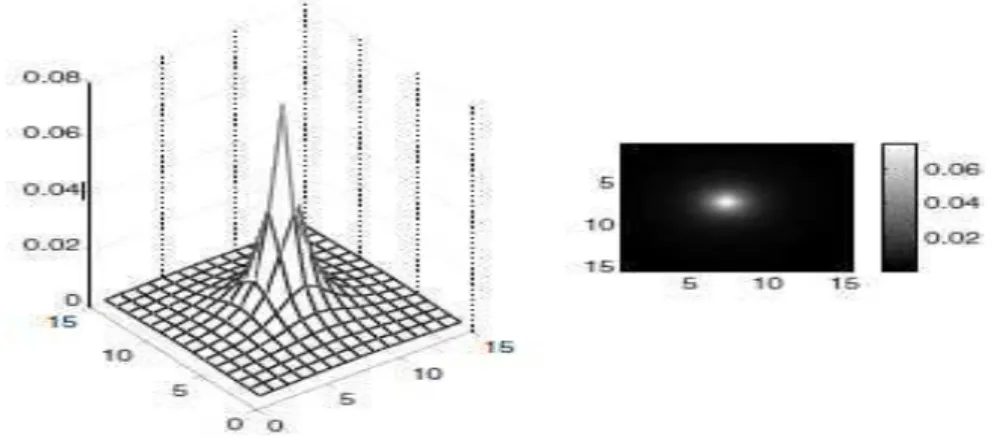
In the following experiments we apply the above algorithms for the restoration of the camerama image. We assume that the blur kernel is a 15 x 15 filter with values 1/( + • + 1) for -7 ≤ i; j ≤ 7, normalized to have a unit sum. This blur kernel is shown in Figure 4. We start by presenting the deblurring performance for C = 2 (λ = 0:075).
ISSN 2277-1956
/V1N3-1494-1503
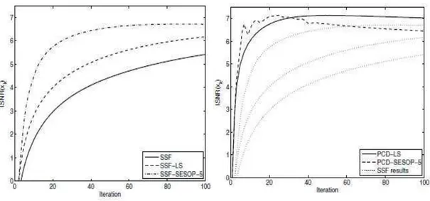
Fig. 4. The value of the penalty function in Equation 2 as a function of the iteration, shown for several iterative-shrinkage algorithms: (i) Plain SSF; (ii) SSF boosted by a line-search; (iii) PCD (with line-search); (iv) SSF with SESOP speedup; and (v) PCD with SESOP
speedup.
Figure 4 presents the comparative performance of the SSF (plain, with line-search, andwith SESOP-5 acceleration) and the PCD (regular and with SESOP-5 too). The graphs show the value of the objective as a function of the iteration. It is clear that (i) line-search is helpful for SSF; (ii) SESOP acceleration helps further in accelerating SSF and PCD; and (iii) PCDSESOP- 5 is the fastest to converge. For a quantitative evaluation of the results, we use the Improvement-Signal-to- Noise Ratio (ISNR) measure, defined as
Go• = 10 log ”‖~ X1Ž‖ ‖Ž1ŽX‖ • [db] (21)
This way, if we propose Xas the solution, ISNR = 0dB. For a restored image of better quality, the ISNR is expected to be positive, and the higher it is, the better the image quality obtained.
ISSN 2277-1956
/V1N3-1494-1503
Figure 5shows the ISNR results for the test with C = 2, as a function of the iteration for the various iterative-shrinkage algorithms tested. As can be seen, PCD (with or even without a SESOP speedup) is the fastest to obtain the maximal quality.
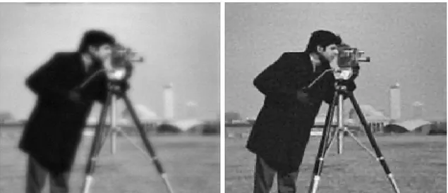
Fig. 6. Deblurring results with 30 iterations of the PCD algorithm: Measured blurry and noisy image (left), and restored (right). This result refers to the experiment with C = 2 (resulting with IS NR = 7:05dB).
Figure 6shows the restored images obtained after 30 iterations of the PCD algorithm. Figure 7 similarly shows the result obtained for C = 8 (for which we choose λ = 0.15 for best ISNR). As can be seen, the resulting images are restored very well, even by this very simple and crude algorithm.
Fig. 7. Deblurring results with 30 iterations of the PCD algorithm and MMSE Estimator : Measured blurry and noisy image (left), and restored (right). This result refers to the experiment with C = 8 (resulting with IS NR = 5:17dB).
10. Conclusion
ISSN 2277-1956
/V1N3-1494-1503
References
[1] Gonzalez, Woods, “Digital Image Processing” Prentice Hall of India, second edition, 813 pages.
[2] Alexander Jung, Z Ben-Haim, Franz Hlawatsch, and Y.C. Eldar, (2011) “Unbiased Estimation of a Sparse Vector in White Gaussian Noise”, IEEE Transaction on Information Theory, CLN 10-489, July,2011.
[3] Antonin Chambolle, Ronald A. DeVore, Nam-yong Lee and Bradley J. Lucier, (1998) “Nonlinear Wavelet Image Processing: Variational Problems, Compression, and Noise Removal through Wavelet Shrinkage”.
[4] Caroline Chaux, Patrick L.Combettes, Jean-C Pesquet and Valerie R. Wajs, (2006) “Iterative Image Deconvolution using Overcomplete Reprsentations”.
[5] David L.Donoho, (1995) “De-Noising by Soft-Thresholding”, IEEE Transaction on Information Theory, Vol. 41, No. 3, May 1995. [6] Fadili M.J. and Starck J.-L., (2007) “Sparse Representation-based Image Deconvolution by Iterative Thresholding”.
[7] Hanjie Pan and Thierry Blu, (2010) “Sparse Image Restoration using Iterated Linear expansion of Thresholds”.
[8] Jean-Luc Starck, Emmanuel J. Candes and David L. Donoho, (2002) “Curvelet Transform for Image Denoising”, IEEE Transaction on Image Processing, Vol.11,No.6,June 2002.
[9] Jose M. Bioucas-Dias, Mario A.T. Figueiredo and Robert D. Nowak, (2007) “Majorization–Minimization Algorithms for Wavelet-Based Image Restoration”, IEEE Transaction on Image Processing,vol.16(12),pp.2980–2991, Dec 2007.
[10] Jose M. Bioucas-Dias Mario A. T. Figueiredo, (2006) “An Iterative Algorithm for Linear Inverse Problems with Compound Regularizers”. [11] Mario A.T Figueiredo, Robert D.Nowak, (2000) “An EM Algorithm for Wavelet-Based Image Restoration”, IEEE Transaction on Image
Processing, vol.12(8), pp.906–916, 2003.
[12] Matan Protter, Irad Yavneh and Michael Elad, (2008) “Closed-Form MMSE Estimation for Signal Denoising Under Sparse Representation Modeling”, IEEE 25-th Convention of EEE in Israel, Dec 2008.
[13] Mario A. T. Figueiredo and Robert D. Nowak, (2005) “Blind Deconvolution of Images using Optimal Sparse Representations”, IEEE Transaction on Image Processing, 2004.
[14] Michael Elad, Boaz Matalon, Michael Zibulevsky, (2006) “Image Denoising with Shrinkage and Redundant Representations”. [15] Michael Elad and Michal Aharon, (2010) “Image Denoising Via Learned Dictionaries and Sparse Representation”.
[16] Michael Elad, M´ario A.T. Figueiredo and Yi Ma, (2010) “On the Role of Sparse and Redundant Representations in Image Processing”, Proceedings of IEEE-Special issue on Application of Sparse Representation and Compressive Sensing.
[17] Raja Giryes,Michael Elad and Yonina C. Eldar, (2009) “Automatic Parameter Setting for Iterative Shrinkage Methods”.
[18] Ron Rubinstein, Alfred M. Bruckstein and Michael Elad, (2010) “Dictionaries for Sparse Representation Modelling”, IEEE Transaction on Image Processing, 2010.
[19] Ron Rubinstein, Michael Zibulevsky and Michael Elad, (2010) “Double Sparsity: Learning Sparse Dictionaries for Sparse Signal Approximation”, IEEE Transaction on Signal Processing, 2010.
[20] Steven Lansel, Manu Parmar and Brian A. Wandell, (2009) “Dictionaries for Sparse representation and Recovery of Reflectances”, Proceedings of SPIE-IS&T Electronic Imaging SPIE Vol.7246,72460D-2009.
[21] Yifei Lou, Andrea L. Bertozzi and Stefano Soatto, (2011) “Direct Sparse Deblurring”, J Math Imaging Vis 39: 1–12.
[22] Yilun Wang, Wotao Yin and Yin Zhang, (2007) “A Fast Algorithm for Image Deblurring with Total Variation Regularization”, CAAM Technical Report (TR07-10) 2007.
[23] Zhangzhang Si and Ying Nian Wu, (2010) “Wavelet, Active Basis, and Shape Script- A Tour in the Sparse Land”. [24] Zhe Hu, Jia-Bin Huang and Ming-Hsuan Yang, (2007) “Single Image Deblurring with Adaptive Dictionary Learning”.