A Unified Approach to Parallel Programming
Victor Eijkhout
Abstract—We propose a new theoretical model for par-allelism. The model is explictly based on data and work distributions, a feature missing from other theoretical models. The major theoretic result is that data movement can then be derived by formal reasoning. While the model has an immediate interpretation in distributed memory parallelism, we show that it can also accomodate shared memory and hybrid architectures such as clusters with accelerators.
The model gives rise in a natural way to objects appearing in widely different parallel programming systems such as the PETSc library or the Quark task scheduler. Thus we argue that the model offers the prospect of a high productivity programming system that can be compiled down to proven high-performance environments.
Index Terms—Parallel programming, DAG model, dis-tributed memory
I. INTRODUCTION
A
S computer architectures become larger in scale and more sophisticated in their hybrid nature (cluster, shared memory, accelerators), the problem of high productiv-ity high performance programming is becoming acute. The problem is only to a limited extent one of the low level programming models: the major part of the problem is the parallel coordination of cores, devices, cluster nodes, co-processors, et cetera.Solutions such as CUDA or MPI have any number of limitations, foremost among which that they are all special purpose, so it is not possible to write a code that is portable between systems. Also, such programming systems are often of a low level, asking the programmer to be concerned with details that are not essential to the application.
In this paper we give the design of a system that takes an abstract approach to implementing parallel algorithms where specific architectural details can be explicitly modeled. Our Integrative Model for Parallelism (IMP) allows for an abstract description of an algorithm, that can be made explicit through successive transformations, one of which being its convolution with an abstract description of hardware.
Specifically, the IMP model is based on kernels, which correspond to parallel tasks without data dependencies. From the distribution of work and data, data movement is theoreti-cally derived as a first-class object. A single kernel typitheoreti-cally corresponds to a collective operation, or a bulk data transfer such as exists in the PETSc [1] and Trilinos [2] libraries.
By composing IMP kernels we arrive at an ‘abstract algorithm’, which is takes the form of a directed acyclic graph (DAG) or dataflow diagram. Actual data motion results from an assignment of tasks to ‘computing locales’: threads, cores, nodes, et cetera. The strength of the IMP model is that this assignment is again an explicit feature of the model, so data motion becomes derivable from the abstract algorithm,
Manuscript received July 18, 2012
V. Eijkhout is with the Texas Advanced Computing Center (TACC) of The University of Texas at Austin. E-mail:[email protected]
rather than being explicitly coded as MPI messages, or implicitly resulting as side-effect of the execution. We will explain this in detail, and give motivating examples.
Having an explicit data motion object has several ad-vantages: for one, it means that a programmer does not have to code in terms of send/receive. For another, the same communication pattern is often used several times in a row. Thus, having a data motion object allows for any preprocessing for optimizing the communication schedule to be amortized. This is known as the ‘inspector-executor’ model [3].
A few things our model is not. It is a programming model, so we offer no transformations of existing codes. It is not a cost model, though cost can be included in our formal derivations. We do not propose a new programming language: we feel that high performance can be reached by compiling down to already existing tools. We do not claim to be able to derive optimal algorithms, routing, or scheduling: the programmer still has the responsibility for the algorithm design; we offer a high level, high productivity way of expressing the design.
II. THE BASICI/MPMODEL
In this section we develop the basic theoretical framework of the IMP model.
A. Basics
We define akernelin the IMP model as a directed bipartite graph, that is, a tuple comprising an input data set, an ouput data set, and a set of elementary computations that take input items and map them to output items:
A=hIn,Out, Ei
whereIn,Out are data structures, and E is a set of (α, β)
elementary computations, where α ∈ In, β ∈ Out and ‘elementary computations’ are simple computations between a single input and output. This is a restriction that we will address in section II-C.
To parallelize a kernel overP processors, we define
A=hA1, . . . , APi, Ap=hInp,Outp, Epi,
describing the parts of the input and output data set and (crucially!) the work that are assigned to processor p. The only restrictions on these distributions are
In =[
p
Inp,Out = [
p
Outp, E= [
p
Ep;
relations in processor locality between input/output data sets and elementary computations.
Based on the fact that the computations inEpare executed on processorpwe can now define the input and output data for these computations:
In(Ep) ={α: (α, β)∈Ep},
Out(Ep) ={β: (α, β)∈Ep}.
These correspond to the input elements that are needed for the computations on processor p, and the output elements that are produced by those computations. These sets are related toInp,Outpbut are not identical: in fact we can now characterize the communication involved in an algorithm as
In(Ep)−Inp data to be communicated to pbefore computation onp
Out(Ep)−Outp data computed on p, to be communicated out afterwards
We see that with this basic model we have managed to capture simple message passing: if(α, β)∈Epandα∈Inq (andα6∈Inp) then a message needs to be sent from processor
q top. We will now expand this basic model.
B. From kernels to algorithms
Above we defined the concept of a parallel kernel. By composing multiple kernels we arrive an ‘abstract algo-rithm’: a description of data dependencies between parallel processes, but without regard for architectural details. This corresponds to the much-studied dataflow model where a task can start (‘fire’) if all of its inputs are available, which is when the earlier tasks have finished; see for instance [4].
As a notation for multiple kernels we use superscripts to identify the proper sets. Ifσandτare two kernels we denote them formally as
Aσ=hInσ,Outσ, Eσi, Aτ =hInτ,Outτ, Eτi.
We now have several ways of denoting kernel composition. For simple comosition we can write y = τ(σ(x)) or y = τ ◦ σ(x). Interpreting the Eσ, Eτ edge sets as functional mappings from their inputs to their outputs we also write
Outτ ←Eτ ←Eσ(Inσ).
The advantage of this arrow notation is that it becomes easy to express graphically a DAG of kernels1: one kernel
can feed into more than one, breaking the linearity of simple composition.
Finally, if for each kernel we draw up the adjacency matrix we find a linear algebra description of the abstract algorithm:
Outτ=Aτ·AσInσ,
whereAσ, Aτ are the adjacency matrices of theσ, τ opera-tions, andInσ,Outτ are rendered as vectors.
1Note: this is not the DAG of tasks that appears in much current research,
for which see later.
C. Normal form
We defined the edges in an IMP kernel to map a single input to a single output, which could be restrictive. We solve this by recognizing that the integration of computation and data movement in the elementary computations of a kernel does not exist in practice: communication and computation are separate activities. Thus, we can decompose an IMP kernel into two kernels, where one has arcs that are pure data movement, and one that has pure computation.
• Since we are mostly interested in data movement, the computation kernels will be omitted.
• The objection that arcs might connect subsets ofInor Outdisappears: a computation that has multiple inputs (and for instance combines them on the target) can be split into multiple arcs that simply move data, followed by a combination on the target task.
III. DISTRIBUTIONS
The model as explained so far incorporates distributed data. We will now introduce distributions as formal entities. One justification for this is that the partitioningp7→Inp is obviously a distribution, but p7→ In(Ep) is also one. The former is often disjoint; the latter commonly not. Thus, the transformation from one distribution to another is also an important aspect of our model. Also, formulating algorithms in terms of distributions lifts the interpretation of the model from simple message passing to a more global description.
Let us consider a vector2 of size N and P processors.
A distribution is a function that maps each processor to a subset of N. We make the common identification of N = {0, . . . , N−1}andP ={0, . . . , P−1}; likewiseNM is the set of mappings fromM toN, and thereby2N is the set of mappings from N to{0,1}; in effect the set of all subsets of{0, . . . , N −1}. A distribution is then
v:P →2N.
Thus, each processor stores elements of the vector; the partitioning does not need to be disjoint.
A couple of examples. With β = N/P (assuming for simplicity’s sake thatN is evenly divisible byP) we define the block distribution
b≡p7→[pβ, . . .(p+ 1)β−1], (1)
the cyclic distribution
c≡p7→ {i: mod (i, β) =p},
and the redundant replication
∗ ≡p7→N.
Finally, we consider the ‘natural’ distribution
↑≡p7→[f(p), . . . , f(p+ 1)−1]
where f(p) is the number of elements stored on proces-sors 0. . . p−1. If this distribution is induced by another distribution u, meaning that f(p) = |u(p)|, we denote this asu↑.
2We can argue that limiting the exposition to vectors is no limitation, as
Let x be a vector and v a distribution, then we can introduce an elegant, though perhaps initially confusing, notation for distributed vectors:
x(v)≡p7→x[v(p)]
That is, x(v) is a function that gives for each processor
p the elements of x that are stored on p according to the distributionv. As an important special case, x(∗)describes the case where each processor stores the whole vector.
As observed above, the most important application of distributions is converting a vector between one distribution and another. We use the notationT(u, v)for this conversion, so
x(v) =T(u, v)x(u). (2)
A. The software context
Distributions can be used in software as follows. Suppose we are adding an kernelK with input xand outputy in a code segment where certain distributions hold:
... code ...
{ x is distributed as x(u) }
// the operation mapping x->y goes here { y is distributed as y(v) }
... code ...
Suppose the kernel is defined as K = hx(u′), y(v′), EKi, then we need to surround the kernel by transformations T
according to equation (2):
{ x is distributed as x(u) } x(u’) = T(u,u’) x(u)
// apply the kernel on x(u’), giving y(v’) y(v’) = T(v’,v) y(v)
{ y is distributed as y(v) }
B. Composing distributions
If v andw are distributions, we can compose them, and indicate the relationship of the composition to the constituent parts:
x(w)≡p7→x(v)[v−1◦w(p)]
This means that we can describexdistributed according tow
in terms of the v distribution, involving the communication described as v−1 ◦ w. We also denote this conversation
between distributions as T(v, w).
Example.: Let x be distributed as x(v). To transform it to x(∗), we need to move data accoording to v−1◦ ∗.
v−1◦ ∗(p) =v−1(N) =P.
After all this complication about composing distributions, we note that often we do not ‘track’ data through multiple redistributions: we take one distribution for given and only consider a single redistribution. After this, the resulting distribution is again interpreted as a natural redistribution, to be redistributed further again. This is modeled by the object
T(u, u↑).
C. Sparse distributions
For dealing with irregular data access we extend the distribution notation further. LetGbe an boolean adjacency matrix, and define
G(i)≡Gi≡ {j:gij6= 0}
which can be justified by interpreting the matrix as a row list of column lists of nonzero positions. For example, with a tri-diagonal matrix we haveG(i) ={i−1, i, i+ 1}.
This adjacency matrix can be used to transform distribu-tions: with
u:p7→u(p)∈2N
we define
Gu≡p7→ ∪i∈u(p)Gi∈2N (3)
In the tridiagonal example, and using the block distribution of equation (1), we have:
(
letu0, u1 be s.t.u(p) = [u0, . . . , u1], thenGu(p) = [u0−1, . . . , u1+ 1].
The justification for such transformations on distribution is for irregular data access, such as in the sparse matrix-vector product. With u describing p 7→ Inp, and G the sparsity pattern of the matrixA,Gu corresponds toIn(Ap).
IV. EXAMPLES
We will show two examples of how algorithms are ex-pressed and analyzed in the IMP model.
A. Matrix-vector product
As a simple example we consider the dense matrix-vector product. There are several ways of implementing this algo-rithm, such as with the matrix distributed by rows, columns, or blocks (see for instance [5]), and each of the three variants requires a radically different implementation. In this section we show that it is possible to formulate the algorithm on a high level, such that data traffic is automatically correctly derived.
We split the computation into two I/MP kernels3,
cor-responding to computation of temporaries and subsequent reduction:
∀i:yi=Pjaijxj
=P
jtij, tij=aijxj.
For an I/MP kernel we need to distribute data and work. For the data we use some distributionufor both input and output. The work distribution is induced by the decision that
tij is computed whereaij lives.
We now consider the product by rows. In distribution notation the algorithm is:
(
t(v,∗)←A(v,∗)x(∗) y(v)←P
jt(v,∗). and we reason as follows:
• A(v,∗)describes the distribution ofAby rows. • xis distributed on input asx(v), so transforming it to
x(∗)is an allgather.
3We only discuss 1D distributions; 2D is possible with slightly more
• t(v,∗) is correctly distributed for the reduction, so no communication is needed there.
• y(v)is the resulting distribution as desired.
For the product by columns we reason similarly. First of all, we express the algorithm in distribution notation:
(
t(∗, v)←A(∗, v)x(v) y(v)←P
jt(v,∗).
The differences in reasoning are thatxis correctly distributed as x(v) on input, so no communication is needed here. On the other hand, the output of the first stage t(∗, v) is not correctly distributed for the reduction, and we conclude that a data transposition is needed.
The conclusion from this simple example is that it is possible to describe the algorithm on a high level, with a Matlab-like global notation, while the communication is formally derived from the distributions on the data.
B. N-body problems
Algorithms for the N-body problem need to compute in each time step the mutual interaction of each pair out of N particles, giving an O(N2) method. However, by
suitable approximation of the ‘far field’ it becomes possible to have anO(NlogN)or even anO(N)algorithm, see the Barnes-Hut octree method [6] and the Greengard-Rokhlin fast multipole method [7].
The naive way of coding these algorithms uses a form where each particle needs to be able to read values of in principle every cell. This is easily implemented with shared memory or an emulation of it. Pseudo-code would look like:
parallel over all particles p: cell-list = all top level cells sequential over c in cell-list:
if c is far away, evaluate forces p<->c otherwise
open c and add children to cell-list
However, this algorithm can be implemented just as easily in distributed memory, using message passing [8]. To show that an implementation can be formally derived we consider the following form of the N-body algorithms (see [9]):
• The field due to cellion levelℓ is given by
g(ℓ, i) =⊕j∈C(i)g(ℓ+ 1, j)
where C(i) denotes the set of children of cell i and ⊕stands for a general combining operator, for instance computing a joint mass and center of mass;
• The field felt by cell ion levelℓis given by
f(ℓ, i) =f(ℓ−1, p(i)) + X
j∈Iℓ(i) g(ℓ, j)
where p(i) is the parent cell of i, and Iℓ(i) is the interaction region of i: those cells on the same level (‘cousins’) for which we sum the field.
1) Kernel implementation: We can model the above for-mulation straightforwardly in terms of IMP kernels: the g
computation hasE(g)=Eτ∪Eγ, where (
Eτ={τℓ ij}
Eγ ={γℓ i}
,
(
∀i∀j∈C(i): τijℓ =‘tℓij =gℓj+1 ’ ∀i: γiℓ=‘giℓ=⊕j∈C(i)tℓij ’
(4)
Thetℓ
ijquantities are introduced so that their assignment can model data communication: as in the matrix-vector example above, thegℓ
i reduction computation is then fully local. Similarly, thef computation isE(f)=Eρ∪Eσ∪Eφ∪Eη, where
Eρ={ρℓ i}
Eσ={σℓ ij}
Eη={ηℓ i}
Eφ={φℓ i}
,
∀i: ρℓi=‘riℓ=fℓ −1
p(i) ’
∀i∀j∈Iℓ(i): σijℓ =‘sℓij =gℓj ’ ∀i: ηiℓ=‘ hℓi =
P
j∈Iℓ(i)sℓij ’ ∀i: φℓi =‘ fiℓ=rℓi+hℓi ’
(5) These formulations can immediately be translated to a mes-sage passing implementation.
Transformations of the algorithm are possible. For in-stance, in the statement
∀i∀j∈Iℓ(i): sℓij=gjℓ
we recognize a broadcast of gℓ
j to all nodes i such that
j∈Iℓ(i). We can reformulate it as such by exchanging the quantifiers:
∀j∀i∈Jℓ(j):sℓij =gjℓ
where
Jℓ(i) ={j: j∈Iℓ(i)}.
2) Distribution implementation: Instead of individual message passing, we can derive an implementation using distributions. Consider for instance the g calculation of equation (4)
(
∀i∀j∈C(i): τijℓ =‘tℓij =gℓj+1 ’ ∀i: γiℓ=‘giℓ=⊕j∈C(i)tℓij ’
As in section III-C we define an adjacency matrixAfor this operation by
Ai={j: j∈C(i)}.
Now letg be distributed with some distributionu, thentis distributed as t(Au), and summing the tℓ
ij terms is then a local operation.
3) Practical aspects: We have here given two imple-mentations of tree algorithms for N-body problems. Both implementations can cope with the difficulties that distributed memory imposes; as indicated above, shared memory im-plementations are considerably easier to describe. However, our implementations essentially give a dependency graph of tasks, hence they can also serve as shared memory implementations.
In the distributed memory case we invoke the inspector-executor paradigm (see the introduction): we determine which elements need to communicate, in particular theIℓ(i) andCℓ(i)sets, and use this information to evaluate irregular gathers repeatedly.
direct applicability to distributed memory parallel computing with an interconnect that is essentially all-to-all, such as a fat-tree.
However, in other circumstances it fails to account for several aspects:
• A distributed memory architecture can have a mesh interconnect, or other scheme where certain processor pairs do not have a direct connection.
• In a cluster with accelerators the accelerators do not connect to the network but only to a host processor. • The model does not suggest any scheduling for
opera-tions, and the available parallelism can greatly exceed the number of physically available processors.
• In shared memory, using threading, several processes live in the same physical address space. In this case, cer-tain data dependencies correspond to a data movement no-op; also, the precise timing of tasks then becomes an issue.
In order to cover these aspects we need to include some more machinery in the IMP model. First of all, we introduce ‘abstract implementations’: abstract algorithms where each task receives a time stamp and is bound to a computing locus, an abstraction that will cover cores, nodes, et cetera. Formally:
B=hV, E, p, ti where (
p:V →P
t: V → {t0, t1, . . .}
It is easy to associate an abstract implementation with an abstracct algorithm. Let A =AK◦ · · · ◦A1 be an abstract
algorithm consisting of K kernels. We express this in the form of a DAG:
A=hV, Ei,
(
V ={(k, i) :k= 1. . . K, i= 1. . .|Outk|}
E=∪kEk
(6) and one abstract implementation is found by associating vertex(k, i)with time kand locus i.
We call this type of graph an abstract implementation, since we still ignore various practical considerations:
• Arcs in this graph correspond to data movement, but they can take the form of a no-op, a cache miss, data copy, or an MPI message. We will later consider how this difference can be formalized.
• The abstract implementation can ask for more processes than there are processors, so an extra layer of mapping is needed.
Thus, we need to introduce transformations on abstract implementations in order to arrive at ‘realizable implementa-tions’: abstract implementations that satisfy, or are optimized for, real-world constraints. We will do this algebraically, by applying transformations to the adjacency matrices, as explained in section II-B.
Finally, we describe how the realization properties of a realizable implementation can be derived formally: this step is necessary to account for such facts as that on-node MPI communication do not involve network traffic.
Discussion: The above transformations on adjacency
graphs accomplish much the same as DAG schedulers such as Quark [10]. In fact, our transformations do not constitute a schedule optimization strategy. Finding such a strategy may
be NP-complete [11], and static scheduling does not account for machine and OS ‘noise’. Thus, the main point of this section is to illustrate how the IMP model can derive the DAGs that can then be scheduled by other means.
We will now show two examples of reasoning about abstract implementations.
A. Derivation of physical data movement
Applying our model to distributed memory with one process per processor, each data dependency corresponds uniquely to one phyisical data transfer. In architectures that feature multi-threading, shared memory cluster nodes, or co-processors, this is no longer the case. In this section we develop the mechanisms of deriving physical data movement from abstract data dependencies by considering two exam-ples where the process-to-processor assignment mapping is not one-to-one.
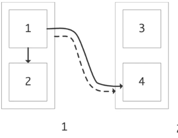
Shared memory cluster nodes: We start with a common
example of distributed memory clusters where each node supports multiple processes that live on shared memory. This is illustrated in figure 1, where we have two cluster
Fig. 1. Communication between processes (solid) and nodes (dotted) in a cluster/shared memory architecture
nodes with two shared memory processes each. In this case, algorithm edges(1,2)or(3,4)do not need an MPI message, while edges such as(1,4)do.
Thus, we have two graphs: the process graph from the IMP kernel, connecting four processes, and the resulting processor graph, connecting two processors. We derive the latter from the former by a linear transformation. Let us consider specifically the IMP dependencies in figure 1.
First we form the embedding operator from the processes to the cluster nodes
I4 2 =
⋆ ⋆ · ·
· · ⋆ ⋆
that reflects that the first two processes live on node 1, while the third and fourth live on node 2. We denote its transpose byI2
4.
The process edge(1,4)in the figure can now be rendered with an adjacency matrix
G4=
· · · · · · · · · · · ·
⋆ · · ·
If we now form the product
G2=I24·G4·I42=
· ·
⋆ ·
we get the correct description of communications in terms of cluster nodes.
However, there is a conceptual problem with this. If we consider the intra-node edge (1,2), its transform becomes
G4=
· · · ·
⋆ · · ·
· · · · · · · ·
⇒G2=I4
2 ·G4·I42=
⋆ · · ·
stating that a message from node 1 to node 1 is required. Therefore, we introduce an extra term and form
(I24·G4)⊛I24=
· · · ·
⋆ · · ·
whereA⊛B is the element-by-element computation ofa⊛ b ≡ a∧ ¬b. The ⊛-multiplication by I24 has the effect of
limiting the communication description to only processes that are on different processors. Redoing the above examples we now find the same G2 matrix for the inter-node case, and
G2=
· · · ·
for the intra-node case, indicating that no MPI communica-tion is needed.
Redundant processes: Next we consider redundant
assignment of one process to two processors. As a specific example we take a domain decomposition method with two subdomains and one separator. In the forward sweep of the system solution the separator collects data from the subdomains; in the backward sweep it distributes data to them. We model this process by three processes, mapped to two processors, with the separator process redundantly assigned to both physical processors.
This process is illustrated in figure 2. In the left column we have the structure of the forward sweep. The algorithmic
Fig. 2. Communication between logical and physical processors in the forward and backward sweep
data movement (top) takes the form of data send from the subdomains 1 and 2 to the separator 3, and the corresponding physical data movement (bottom). Since process 1 sends data to process 3, which is redundantly run on processor 2, there is a message from 1 to 2, and vice versa.
In the backward sweep, process 3 sends data to both 1 and 2, but now, since process 3 is redundantly run on both processors 1 and 2, this data movement is purely local to the processor, requiring no message passing.
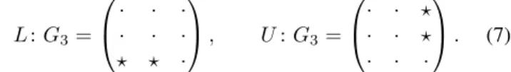
We model this algebraically as follows. The forward and backward sweep are IMP kernels, which we represent by
their adjacency matrices. These describe data movement between processes, that is, the algorithmic data movement:
L:G3=
· · · · · ·
⋆ ⋆ ·
, U:G3=
· · ⋆
· · ⋆
· · ·
. (7)
The matrix embedding the logical processes in physical processors isI3
2 and byI32we denote its transpose. We can
now derive the matrix of physical communications as
G2= (I23·G3)⊛I23
·I32
similar to the previous example.
If we go through this calculation for the operators in equation (7), we find
L:G2=
· ⋆
⋆ ·
, U:G2=
· · · ·
(8)
reflecting the above described behaviour that in theLsweep the processors have to exchange data, but not in theUsweep.
VI. CONCLUSION
In this paper we have presented the Integrative Model for Parallelism which offers a mode of describing parallel algo-rithms that is high-level and expressed in global terms Since data movement (such as message passing in a distributed memory context) is formally derived in the model, rather than explicitly coded it offers two prospects:
• Algorithm expression is expressed independent of any particular machine model, so we can achieve portability over architecture types; and
• since data movement is derived rather than coded, we may achieve higher programmer productivity.
Additionally we have shown how architectural features can explicitly be accomodated in this model.
REFERENCES
[1] W. D. Gropp and B. F. Smith, “Scalable, extensible, and portable numerical libraries,” inProceedings of the Scalable Parallel Libraries Conference, IEEE 1994, pp. 87–93.
[2] M. A. Heroux, R. A. Bartlett, V. E. Howle, R. J. Hoekstra, J. J. Hu, T. G. Kolda, R. B. Lehoucq, K. R. Long, R. P. Pawlowski, E. T. Phipps, A. G. Salinger, H. K. Thornquist, R. S. Tuminaro, J. M. Willenbring, A. Williams, and K. S. Stanley, “An overview of the trilinos project,”
ACM Trans. Math. Softw., vol. 31, no. 3, pp. 397–423, 2005. [3] A. Sussman, J. Saltz, R. Das, S. Gupta, D. Mavriplis, and R.
Pon-nusamy, “Parti primitives for unstructured and block structured prob-lems,” 1992.
[4] R. M. Karp and R. E. Miller, “Properties of a model for parallel computations: Determincay, termination, queueing,” SIAM j. Appl Math., vol. 14, pp. 1390–1411, 1966.
[5] G. Stewart, “Communication and matrix computations on large mes-sage passing systems,”Parallel Computing, vol. 16, pp. 27–40, 1990. [6] J. Barnes and P. Hut, “A hierarchical O(N log N) force-calculation algorithm,”Nature, vol. 324, pp. 446–449, 1986. [Online]. Available: http://dx.doi.org/10.1038/324446a0
[7] L. Greengard and V. Rokhlin, “A fast algorithm for particle simula-tions,”J. Comput. Phys., vol. 73, p. 325, 1987.
[8] J. K. Salmon, M. S. Warren, and G. S. Winckelmans, “Fast parallel tree codes for gravitational and fluid dynamical n-body problems,”Int. J. Supercomputer Appl, vol. 8, pp. 129–142, 1986.
[9] J. Katzenelson, “Computational structure of the n-body problem,”
SIAM Journal of Scientific and Statistical Computing, vol. 10, pp. 787–815, July 1989.
[10] A. YarKhan, J. Kurzak, and J. Dongarra, “QUARK users’ guide: Queueing and runtime for kernels,” University of Tennessee Innovative Computing Laboratory, Tech. Rep. ICL-UT-11-02, 2011.