Par@Graph – a parallel toolbox for the construction and analysis of large complex climate networks

(1)

GMDD

8, 319–349, 2015

Par@Graph

H. Ihshaish et al.

Title Page

Abstract Introduction

Conclusions References

Tables Figures

◭ ◮

Back Close

Full Screen / Esc

Printer-friendly Version Interactive Discussion

Discussion

P

a

per

|

Discussion

P

a

per

|

Discussion

P

a

per

|

Discussion

P

a

per

|

Geosci. Model Dev. Discuss., 8, 319–349, 2015 www.geosci-model-dev-discuss.net/8/319/2015/ doi:10.5194/gmdd-8-319-2015

This discussion paper is/has been under review for the journal Geoscientific Model Development (GMD). Please refer to the corresponding final paper in GMD if available.

Par@Graph – a parallel toolbox for the

construction and analysis of large

complex climate networks

H. Ihshaish1,3, A. Tantet2, J. C. M. Dijkzeul1, and H. A. Dijkstra2

1

VORtech – scientific software engineers, Delft, the Netherlands

2

Institute for Marine and Atmospheric research Utrecht, Utrecht University, Utrecht, the Netherlands

3

Department of Computer Science and Creative Technologies, UWE-Bristol, UK

Received: 23 November 2014 – Accepted: 16 December 2014 – Published: 20 January 2015

Correspondence to: H. Ihshaish (hisham.ihshaish@uwe.ac.uk)

Published by Copernicus Publications on behalf of the European Geosciences Union.

(2)

GMDD

8, 319–349, 2015

Par@Graph

H. Ihshaish et al.

Title Page

Tables Figures

◭ ◮

Back Close

Full Screen / Esc

Discussion

P

a

per

|

Discussion

P

a

per

|

Discussion

P

a

per

|

Discussion

P

a

per

|

Abstract

In this paper, we present Par@Graph, a software toolbox to reconstruct and analyze complex climate networks having a large number of nodes (up to at leastO(106)) and of edges (up to at leastO(1012)). The key innovation is an effi_{cient set of parallel} soft-ware tools designed to leverage the inherited hybrid parallelism in distributed-memory 5

clusters of multi-core machines. The performance of the toolbox is illustrated through networks derived from sea surface height (SSH) data of a global high-resolution ocean model. Less than 8 min are needed on 90 Intel Xeon E5-4650 processors to construct a climate network including the preprocessing and the correlation of 3×105SSH time series, resulting in a weighted graph with the same number of vertices and about 3×106 10

edges. In less than 5 min on 30 processors, the resulted graph’s degree centrality, strength, connected components, eigenvector centrality, entropy and clustering coeffi -cient metrics were obtained. These results indicate that a complete cycle to construct and analyze a large-scale climate network is available under 13 min. Par@Graph there-fore facilitates the application of climate network analysis on high-resolution observa-15

tions and model results, by enabling fast network construction from the calculation of statistical similarities between climate time series. It also enables network analysis at unprecedented scales on a variety of diff_{erent sizes of input data sets.}

1 Introduction

Over the last decade, the techniques of complex network analysis have found applica-20

tion in climate research. Many studies were focused on correlation patterns in the atmo-spheric surface temperature (Tsonis and Roebber, 2004; Tsonis et al., 2010; Donges et al., 2009b, 2011, 2009a) and teleconnections (Tsonis et al., 2008). Up to now, the behavior of El Niño (Gozolchiani et al., 2008, 2011; Tsonis and Swanson, 2008; Ya-masaki et al., 2008), the synchronization between diff_{erent spatiotemporal climate} vari-25

(3)

GMDD

8, 319–349, 2015

Par@Graph

H. Ihshaish et al.

Title Page

Tables Figures

◭ ◮

Back Close

Full Screen / Esc

Discussion

P

a

per

|

Discussion

P

a

per

|

Discussion

P

a

per

|

Discussion

P

a

per

|

the sea surface temperature (SST) variability and the global mean temperature (Tan-tet and Dijkstra, 2014) have been investigated. In addition, network tools have also been used to detect the propagation of SST anomalies on multidecadal time scales (Feng and Dijkstra, 2014) and to develop early warning indicators of climate transitions (van der Mheen et al., 2013; Feng et al., 2014).

5

In most studies above so-called interaction networks were used. Here the observa-tion locaobserva-tions serve as vertices and edges (links) are based on statistical measures of similarity, e.g. a correlation coeffi_{cient, between pairwise time series of climate} vari-ables at these diff_{erent locations. Given time series of climate data, represented by} anN×M matrix, whereN is the number of locations and M is the length of data at-10

tributes (daily/monthly values), one then needs to calculate at leastN2/2 correlation values. Such computations become challenging for largeN; for example, with a net-work of 106nodes, this would result in 5×1011 calculations. A further challenge is the memory needed for such a computation. To only keep the calculated matrix in memory for further processing, about 3.7×103 GB of memory is required (consider 8 bytes of 15

memory for each of the 5×1011matrix items), which is not available in the vast majority of current computing platforms.

On the other hand, analyzing the resulting network (graph) is non-trivial and also computationally challenging. Considering a graphG, with V vertices (network nodes) andEedges (links between nodes), a typical step in an algorithm to analyzeGinvolves 20

visiting eachv∈V and its neighborsV ⊂V (the set of vertices connected tov by an edge e∈E), then their consecutive neighbors, and so on. Processing such steps is normally done within a computational complexity of the order ofV and/or E squared or cubed. For example the computation of the clustering coeffi_{cient, which measures} the degree to which its vertices tend to cluster together, has a time complexity of O

25

(|V|3). In practice, there are various available software tools for graph analysis, some providing implementations of single-machine algorithms such as BGL (Mehlhorn and Näher, 1995), LEDA (Siek et al., 2002), NetworkX (Hagberg et al., 2008), SNAP1and

1

Stanford Network Analysis Platform – see http://snap.stanford.edu.

(4)

GMDD

8, 319–349, 2015

Par@Graph

H. Ihshaish et al.

Title Page

Tables Figures

◭ ◮

Back Close

Full Screen / Esc

Discussion

P

a

per

|

Discussion

P

a

per

|

Discussion

P

a

per

|

Discussion

P

a

per

|

igraph(Csardi and Nepusz, 2006). However, the computation of a clustering coeffi_cient

for a network with V =₁₀6 _{would be very challenging, if at all possible, with existing} single-machine software.

The most popular approach to tackle such computational challenges is by exploiting parallelism for both the construction and the analysis of those massive graphs through 5

the design of effi_{cient algorithms for parallel computing platforms. In this regard, some} contributions have been made to the development of algorithms that exploit parallel computing machines such as in The Parallel BGL (Gregor and Lumsdaine, 2005) and CGMgraph (Chan et al., 2005). However, due to structure irregularity and sparsity of real-world graphs, including those built of climate data, there are few parallel imple-10

mentations that are effi_{cient, scalable and can deliver high performance. Other factors} which contribute to this ineffi_{ciency include a manifested irregularity of data} dependen-cies in those graphs, as well as the poor locality of data, making graph exploration and analysis highly dominated by memory latency rather than processing speed (Lums-daine et al., 2007). A recent intent with NetworKit2 has shown a remarkable step to-15

wards providing parallel software tools capable of analyzing large-scale networks. Yet the networks analyzed by this software had at most 4×107edges, which is still lower that what is intended to be studied in climate networks.

On top of that, most of the existing libraries do not address the processing and memory challenges involved in the construction of graphs with large V from statisti-20

cal measures of time series. Indeed most researchers tend to develop their own tools to build correlation matrices beforehand, and thereafter they transform these matrices into appropriate graph data structures that can be handled by the existing libraries of graph analysis. An exception is the software package Pyunicorn3, developed at Pots-dam Institute for Climate Impact Research, that couples Python modules for numerical 25

analysis withigraph. It can carry out both tasks; the construction of climate networks and the analysis of the resulted graphs. However, this software is bounded by the

2

Networkit – see http://networkit.iti.kit.edu.

3

(5)

GMDD

8, 319–349, 2015

Par@Graph

H. Ihshaish et al.

Title Page

Tables Figures

◭ ◮

Back Close

Full Screen / Esc

Discussion

P

a

per

|

Discussion

P

a

per

|

Discussion

P

a

per

|

Discussion

P

a

per

|

single-machine’s memory and speed, making it impossible to construct large-node cli-mate networks and consequently, inappropriate to analyze them.

The networks which so far have been handled in climate research applications had only a limited (at mostO(103) number of nodes. As a consequence, coarse-resolution observational and model data have been used with a focus only on large-scale prop-5

erties of the climate system. This system is, however, known for its multi-scale in-teractions and hence one would like to explore the interaction of processes over the diff_{erent scales. Data are available through high-resolution ocean/atmosphere/climate} model simulations but they lead to networks with at leastO(105) nodes and hence they cannot be reconstructed, neither effi_{ciently analyzed using currently available software.} 10

In this paper, we introduce a complete toolbox Par@Graph designed for parallel computing platforms, which is capable of the preprocessing of large number of cli-mate time series and the calculation of pairwise statistical measures, leading to the construction of large node climate networks. In addition, Par@Graph is provided with a set of high-performance network analyzing algorithms for symmetric multiprocessing 15

machines (SMPs). It is also coupled to a parallellized version ofigraph(Csardi and Ne-pusz, 2006) – a widely used graph-analysis library. The presented toolbox is provided with an easy-to-use and flexible interface which enables it to be easily coupled to any existing graph analysis software.

The rest of the paper is organized as follows. In Sect. 2, we give an overview of 20

the computational challenges associated with the reconstruction of climate networks and their analysis. In Sect. 3, we provide a description of the design of Par@Graph and its parallel algorithms for the construction and analysis of climate networks from climate time series. In Sect. 4, we describe the application of the toolbox to data from a high-resolution ocean model including a performance and scaling analysis. Section 5 25

provides a summary and discussion of the results.

(6)

GMDD

8, 319–349, 2015

Par@Graph

H. Ihshaish et al.

Title Page

Tables Figures

◭ ◮

Back Close

Full Screen / Esc

Discussion

P

a

per

|

Discussion

P

a

per

|

Discussion

P

a

per

|

Discussion

P

a

per

|

2 Climate networks

A common data set of climate observations or model results consists of spatiotemporal grid pointsi,i=_1,_{. . .}_,_N _{at a given latitude and longitude, each having a time series of} a state variable, for example temperature,Ti(tk) of lengthL, withk=1,. . .,L. In order to reconstruct a climate network, some preprocessing tasks are required beforehand, 5

including the selection of grid locations and calculation of anomalies (e.g., removal of a trend and/or a seasonal cycle that might produce strong autocorrelations between diff_{erent locations). Having done this, each grid point is considered to be a node in the} resulting network.

2.1 Network reconstruction

10

To define a link between two nodes, both linear and nonlinear dependencies can be considered. To measure linear correlations between the time series T_i(t_k) and T_j(t_k), the Pearson correlation coeffi_cient_R

i j given by

Ri j=

L

P

k=1

T_i(t_k)T_j(t_k)

s _L

P

k=1

T_i2(t_k) L

P

k=1

T_j2(t_k)

(1)

is widely used (Tsonis and Roebber, 2004). Alternatively, measures of nonlinear corre-15

lation can be used, such as the mutual informationM_{i j}, given by

M_{i j}=X T_i,T_j

P_{i j}(T_i,T_j) log Pi j(Ti,Tj)

Pi(Ti)Pj(Tj)

. (2)

(7)

GMDD

8, 319–349, 2015

Par@Graph

H. Ihshaish et al.

Title Page

Tables Figures

◭ ◮

Back Close

Full Screen / Esc

Discussion

P

a

per

|

Discussion

P

a

per

|

Discussion

P

a

per

|

Discussion

P

a

per

|

similarity between nodesi and j is discussed in Donges et al. (2009a). Whatever the choice, however, a correlation matrix (C) ofN×Nelements is produced, whereCi j=Ri j orC_{i j}=_M

i j, whereN is again the number of grid points.

In many climate applications, one is interested in propagating features, such as the propagation of ocean Rossby waves. Time delayed (time-lagged) relationships that 5

exist between climate variables in diff_{erent geographical locations have also been} ad-dressed by the climate networks approach (Gozolchiani et al., 2008; Berezin et al., 2012; Tirabassi and Masoller, 2013; Feng and Dijkstra, 2014; Tupikina et al., 2014). These are commonly measured by examining the correlation between the time series of two locations relatively shifted in time with respect to one another. Technically this 10

can be done by defining a time-lag interval and computing the correlation measures between the shifted time series (Feng and Dijkstra, 2014). One can also define a time interval, say [tmin,tmax], and then find the value of t in this interval where Ci,j(t) is maximal (Gozolchiani et al., 2008).

Having derived the correlation matrix C, a threshold τ is usually applied to define 15

strong similarities between nodes as “links”. The adjacency matrixAfor the network is then found by

Ai j=Aj i = Θ(Ci j−τ)−δi j, (3)

whereΘ_{is the Heaviside function and}_δ_{is Kronecker delta. If correlation values are to} be considered as weights for the resulted links, the elements ofAafter thresholdingC

20

withτbecome

Ai j=

(

0 C_{i j}< τ,

C_{i j} C_{i j}≥τ. (4)

Note that because C is symmetric, the resulting network is always undirected when

Cis calculated at zero time-lag. However, when time-lagged correlations are studied, directions are added to the links between nodes, reflecting the direction of the shifting 25

of their corresponding time series. If only thresholding is applied, but the values of the correlation matrix are kept, a weighted network will result.

(8)

GMDD

8, 319–349, 2015

Par@Graph

H. Ihshaish et al.

Title Page

Tables Figures

◭ ◮

Back Close

Full Screen / Esc

Discussion

P

a

per

|

Discussion

P

a

per

|

Discussion

P

a

per

|

Discussion

P

a

per

|

2.2 Network analysis

Many properties in climate networks have interesting physical interpretations and hence are required to be computed effi_{ciently. For reference in Sects. 3 and 4, we} list here the most important properties.

– Degree centrality. The degree centralityk_i of a nodei refers to the number of its

5

incident vertices, that is,k_i =_|_N₍_i₎_|_{, where}_N₍_i_{) is the set of vertices adjacent to}_i_.

– Strength centrality. For a weighted network, the strength centrality is given by the

sum of the weights of the edges between the node and its incident vertices.

– Clustering Coefficient. The Watts–Strogatz clustering coeffi_cient_C

i measures the probability that two randomly chosen neighbors of a node are also neighbors 10

(Watts and Strogatz, 1998). This metric is calculated for eachi ∈V by

Ci =

̺_i ki(ki−1)

, (5)

whereki is the number of neighbors ofi and̺i is the number of connected pairs between all its neighbors. Whend indicates the average number ofi’s neighbors in a graph, this metric can be obtained inO(|V|d) time and inO(|V|) space. 15

– Entropy. The Shannon entropy of the incident edges’ weights (Anand and

Bian-coni, 2009) which is given for nodei ∈V by

H(i)=₋ k_i

X

j=1

p_{i j}logp_{i j} ; p_{i j}= wi j ki

P

l=1

wi l

, (6)

wherek_i is the (total) degree of nodei andw_{i j} is the weight of edge(s) between nodesi andj. The computation of the entropy for all nodes in a graph is obtained 20

(9)

GMDD

8, 319–349, 2015

Par@Graph

H. Ihshaish et al.

Title Page

Tables Figures

◭ ◮

Back Close

Full Screen / Esc

Discussion

P

a

per

|

Discussion

P

a

per

|

Discussion

P

a

per

|

Discussion

P

a

per

|

– Eigenvector Centrality. This centrality metric is commonly used to evaluate the

influence of a vertex in a network qualitatively. Unlike degree centrality, which weights every edge equally, the eigenvector centrality assigns relative scores to all vertices in the network based on the concept that edges with high-scoring vertices contribute more to the score of the vertex in question than equal edges with low-5

scoring nodes. As a result, one would find that a vertex having high degree does not necessarily imply a high eigenvector centrality, since its connectivity might be with less important vertices. Equally, a vertex with a high eigenvector centrality is not necessarily highly linked (the vertex might have few but important links). As defined in (Bonacich, 1972), let A=₍_A

i j) be the adjacency matrix of the graph 10

G(V,E), the centrality score (xi) of nodei∈V is then found by

x_i =1

λ X

j∈ki

x_j =1

λ X

j∈V

A_{i j}x_j, (7)

whereki is the set of i’s neighbors, andλis a constant. Note that there could be many eigenvaluesλfor which an eigenvector exists, however, the centrality score is determined by calculating the eigenvector corresponding to the largest positive 15

eigenvalue of the adjacency matrix. This metric is obtained computationally in

O(|V|+_|_E_|_{) time and}_O₍_|_V_|_{) space.}

– Betweenness Centrality. This measure, indicated here by BC(v) is based on

shortest-path enumeration. It is considered one of the more commonly used met-rics to quantify the relative importance of nodes in a graph (Freeman, 1977). To 20

obtain this metric given a graph G(V,E), let σst denote the number of shortest paths between the verticess andt. When the count of those which pass through the nodei isσ_st(i), then the BC(i) is obtained by

BC(i)= X s6=_i₆=_t_∈_V

σ_st(i)

σ_st (8)

(10)

GMDD

8, 319–349, 2015

Par@Graph

H. Ihshaish et al.

Title Page

Tables Figures

◭ ◮

Back Close

Full Screen / Esc

Discussion

P

a

per

|

Discussion

P

a

per

|

Discussion

P

a

per

|

Discussion

P

a

per

|

With the sequential algorithm which has been proposed in Brandes (2001), it can be computed inO(|V|+_|_E_|_{) space and}_O₍_|_V_||_E_|_{) time.}

All these quantities can be obtained using the igraph library for relatively small node networks.

3 Description of the toolbox

5

In practice, the reconstruction and analyses of climate networks are carried out through performing a set of separate tasks, progressively. First, the preprocessing of climate time series occurs, then the correlation matrix is calculated, followed by network con-struction from either the correlation matrix or another graph data structure like an adja-cency matrix, and finally the network is analyzed using the selected graph algorithms 10

library. Contrary to these sequence of computations, Par@Graph is designed to pro-vide end-to-end support for the creation and analysis of climate networks by integrating parallel computing tools to perform all the involved processing effi_{ciently. With attention} at the same time to optimize required computing memory.

Par@Graph is composed of a set of coupled parallel tools designed to leverage 15

the inherited hybrid parallelism in distributed-memory clusters of multi-core (SMPs) machines, using MPI/OpenMP standards. The provided tools are classified into two major software modules, which we refer to as the Network Constructor and the analysis engine, together with additional interfacing tools and wrappers.

3.1 Network constructor

20

(11)

GMDD

8, 319–349, 2015

Par@Graph

H. Ihshaish et al.

Title Page

Tables Figures

◭ ◮

Back Close

Full Screen / Esc

Discussion

P

a

per

|

Discussion

P

a

per

|

Discussion

P

a

per

|

Discussion

P

a

per

|

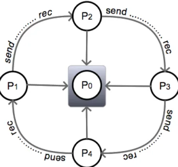
The design of the Constructer follows a master-worker parallel computing paradigm for distributed-memory parallel clusters of SMPs. The calculation of the correlations be-tween time series is distributed over the computing elements (workers), forming a ring topology of processes, shown in Fig. 1, which communicate between each other using MPI standards. As soon as a process findsCi j≥τ, then the pairwise (i,j) are copied 5

to a local process’s buff_{er of a user-configurable size, and sends the iteratively filled} buff_{er to}_p

0, where the network is to be analyzed. Note that if the network is weighted,

the value ofCi,j itself is also copied and sent to the master side by side with its pair of nodesi andj (and in like manner time-lag values).

A brief description of the processing associated to each ring process is described in 10

Algorithm 1 below.

Algorithm 1Network Constructor

1:procedureRINGPROCESS(p) 2: Nlocal←p’s block of time series

3: Nneighbor←neighbor’s block of time series

4: neighbor(right)←p+ 1

5: neighbor(lef t)←p−1

6: preprocessing←remove user specified time cycle

7: performance←reorder time series ofNlocal .for better memory-access

8: local block←cross correlateNlocal .performed once

9: fori←0to(p−1)/2do .iterate half ring 10: functionSEND(Nlocal,neighbor(right)) .send block to a neighbor

11: functionRECEIVE(Nneighbor,neighbor(lef t)) .receive block from another

12: functionC(i,j,8i,j2Nlocal+Nneighbor)

13: if(Ci,j>=τ)then

14: ifweightedthen

15: functionSEND!MASTER(i, j,Ci,j) .time-lagtis also sent to master if needed

16: else

17: functionSEND!MASTER(i, j)

18: neighbor(right)←neighbor(right)+1 19: neighbor(lef t)←neighbor(lef t)-1 20: returnDone

(12)

GMDD

8, 319–349, 2015

Par@Graph

H. Ihshaish et al.

Title Page

Tables Figures

◭ ◮

Back Close

Full Screen / Esc

Discussion

P

a

per

|

Discussion

P

a

per

|

Discussion

P

a

per

|

Discussion

P

a

per

|

Note that only a subsetCofC, such that∀C_i,j ∈C,Ci,j ≥τ, is sent progressively to the master computing element. This indeed means that the under-threshold values of

Care discarded directly at each ring process. This reduces both the amount of data sent to the master element and the memory required there for the construction of the network.

5

The process of constructing the network itself is performed progressively in the events that the master (p0) receives edges’ coordinates (and attributes, e.g.

weights/lags) from any ring process. Initially p0, having the number of dataset grid

points, constructs a completely unconnected network, i.e. no edges between graph vertices. As soon as ring processes start sending edge coordinates top0, these edges

10

are added to the network straightaway. In the long run, constructing the network follow-ing this approach results in savfollow-ing time, since the master is idle (except when receivfollow-ing data from workers) during the ring processing iterations. And more importantly, be-cause the coming edges are added directly to the graph data structure, memory usage is optimized at the master as data redundancy is markedly minimized.

15

With attention to the overall performance, it is crucial not to overlook the I/O over-head, especially because the toolbox is intended to be processing large climate datasets. To that end, the Constructor is designed to perform multiple I/O collective operations at the same time (MPI-IO). In like manner, simultaneously, each ring pro-cess reads its chunk of time series from a parallel file system. Furthermore, owing to 20

the fact that the elements of those time series are neither read nor stored contiguously, another key point in order to improve performance is to optimize memory access at each processor. This is provided at each process by performing preprocessing tasks that include the reordering of each process’s chunk of time series, for the sake of re-ducing cache misses during calculation.

(13)

GMDD

8, 319–349, 2015

Par@Graph

H. Ihshaish et al.

Title Page

Tables Figures

◭ ◮

Back Close

Full Screen / Esc

Discussion

P

a

per

|

Discussion

P

a

per

|

Discussion

P

a

per

|

Discussion

P

a

per

|

3.2 Analysis engine

Once correlations and their coordinates are available at the master machine, it consec-utively runs graph algorithms to analyze the resulted network. The developed parallel algorithms for network analysis are based on those inigraph. The intent here is that this design (coupled with the Network Constructor) will achieve three primary goals: (1) to 5

construct the network rapidly, (2) to enable effi_{cient and safe multithreading of the core} library algorithms and (3) to reduce memory usage for network representation.

With respect to the analyzing algorithms, a set of 20 of the core algorithms ofigraph have been parallelized using POSIX threads and OpenMP directives. Generally speak-ing, the embedded routines of those algorithms (a sample pseudocode is shown below 10

in (a)), could naively be parallelized by transforming their iterative instructions into par-allel loops, see (b) pseudocode:

whilei≤vertices

do

8 <

:

result(i)←some processing

i←i+ 1

(a)

#pragma omp parallel for private(i)

fori←0tovertices,i←i+ +

do

n

result(i)←some processing

(b)

For instance, in a global transitivity routine, by which the network’s average clustering coeffi_{cient is obtained, the value} _result _{is scalar (average value), so that parallelism} 15

appears straightforward and safe multithreading could be achieved by applying reduc-tionbinary operators over its parallelizable loop. Although this may be approachable in similar cases, unfortunately in most routinesresult’s value does not depend linearly on the iteration variablei but in some arbitrary way (depending on the algorithm). This is added to the synchronization overhead which could be imposed in algorithms where 20

dependent iterative operations are found, which need careful consideration to prevent conflicts commonly caused by the concurrent access to shared memory spaces.

(14)

GMDD

8, 319–349, 2015

Par@Graph

H. Ihshaish et al.

Title Page

Tables Figures

◭ ◮

Back Close

Full Screen / Esc

Discussion

P

a

per

|

Discussion

P

a

per

|

Discussion

P

a

per

|

Discussion

P

a

per

|

The parallelized algorithms ofigraphare those mostly used to obtain important net-work metrics needed to evaluate structural (local and global) properties of graphs. Amongst them are the algorithms of shortest paths, centrality measures (e.g., between-ness, closebetween-ness, eigenvector), transitivity and clustering coeffi_{cient, connected} compo-nents, degree and strength centralities, entropy and diameter. A complete list of the 5

parallelized routines and algorithms as well as the particular approach of parallelism for each would make this paper too technical and will be reported elsewhere. However, our approach to achieve effi_{cient fine-grained parallelism for the targeted algorithms}

of igraph included major changes in their internal routines and the used data

struc-tures. For example, shared memory queues were added to achieve safe multithreading, 10

loops’ iterations were optimized to minimize synchronization costs, and iterative work-load was accordingly designed to be scheduled dynamically amongst threads in order to improve load imbalance caused by the poor locality of data. Furthermore, the internal data structure of the graph itself was modified from indexed edge lists (supported by iterators and internal stacks) to graph adjacency lists which resulted in achieving sig-15

nificant reduction of memory requirements, especially in the case of sparse networks. Additionally, special attention was given to the calculation of both the degree and strength centralities. As such, both metrics’ algorithms were redesigned to be com-puted progressively during the time while the network is being constructed. In other words, each time the master receives edges from one of the ring processes, these are 20

added to the accumulated count of the edges that corresponds to their relative ver-tices. As soon as the last packet of edges is received by the master, these metrics are instantly available. A notable benefit of this approach, of course apart from saving time, is the significant reduction of memory requirements, as each time the master receives a new set of edges, the previous ones are released. Such technique enables com-25

(15)

GMDD

8, 319–349, 2015

Par@Graph

H. Ihshaish et al.

Title Page

Tables Figures

◭ ◮

Back Close

Full Screen / Esc

Discussion

P

a

per

|

Discussion

P

a

per

|

Discussion

P

a

per

|

Discussion

P

a

per

|

3.3 Interfaces and other features

In order to match a wider range of user requirements, Par@Graph is provided with all the necessary tools to do the job, including parallel collective tools to write the resulted correlation or mutual information matrices, where each ring process writes its calculated portion to a common file in a parallel file system. This is added to other 5

tools to read (in parallel) and also construct a graph directly from a matrix as well as tools to read and write standard graph formats, including edge lists, adjacency lists and the popularPajekformat which contains metadata added to an edge list.

Another key point is the flexible interface between the Constructor and the analy-sis engine. That is, although the toolbox provides wrappers to the parallelizedigraph, 10

those are quite flexible to be used with any other analysis library instead of igraph, or any other user developed routines. Additionally, users are provided with a configu-ration input file where they can specify their experimental settings. These include the selection of the data grid (location coordinates), preprocessing parameters, the thresh-old, the type of the network (weighted, unweighted, directed, etc), time-lag intervals, 15

whether to construct a network from time series, a matrix or another graph format.

4 Application and performance

In this section, we will apply Par@Graph to reconstruct and analyze networks obtained from high-resolution ocean model data. The motivation for performing these computa-tions is to understand coherence of the ocean circulation at diff_{erent scales (Froyland} 20

et al., 2014).

4.1 The POP model data

The data used here are taken from simulations which were performed with the Parallel Ocean Program (POP, Dukowicz and Smith, 1994), developed at Los Alamos National Laboratory. This configuration has a nominal horizontal resolution of 0.1◦ and is the 25

(16)

GMDD

8, 319–349, 2015

Par@Graph

H. Ihshaish et al.

Title Page

Tables Figures

◭ ◮

Back Close

Full Screen / Esc

Discussion

P

a

per

|

Discussion

P

a

per

|

Discussion

P

a

per

|

Discussion

P

a

per

|

same as that used by Maltrud et al. (2010). We note that this configuration has a tripo-lar grid layout, with poles in Canada and Russia and the model has 42 non-equidistant z-levels, increasing in thickness from 10 m just below the upper boundary to 250 m just above the lower boundary at 6000 m depth. We use data from the control simulation of this model as described in Weijer et al. (2012), where the POP is forced with a re-5

peat annual cycle from the (normal-year) Coordinated Ocean Reference Experiment (CORE4) forcing dataset (Large and Yeager, 2004), with the 6 hourly forcing averaged to monthly.

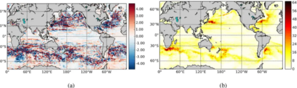
Correlation networks were built from one year (year 136 of the control run) of the simulated global daily sea surface height (SSH) data. The seasonal cycle was removed 10

by subtracting for each day of the year its 5 days running mean averaged over years 131 to 141. The mean and standard deviation of the SSH for this year are plotted in Fig. 2a and b, respectively. Strong spatial and temporal variability can be observed in the region of the western boundary currents (e.g. the Gulf Stream in the Atlantic, the Kuroshio in the Pacific and the Agulhas Current in the Indian Ocean) and the Southern 15

Ocean.

Two datasets have been used for network reconstruction, one with the actual 0.1◦ horizontal resolution of the model, resulting in 4.7×106grid points, and an interpolated one with a lower 0.4◦ horizontal resolution resulting in 3×105 grid points. The latter data set has been used for the performance analysis in the next subsection.

20

4.2 Performance analysis

The results were computed on a bullx supercomputer5composed of multiple “fat” com-puting nodes of 4-socket bullx R428 E3 each, having 8-core 2.7 GHz Intel Xeon E5-4650 (Sandy Bridge) CPUs, with a shared intel smart cache of 20 MB at each socket, resulting in SMP nodes of 32 cores which share 256 GB of memory. The interconnec-25

4

See http://data1.gfdl.noaa.gov/nomads/forms/core/COREv2.html.

5

(17)

GMDD

8, 319–349, 2015

Par@Graph

H. Ihshaish et al.

Title Page

Tables Figures

◭ ◮

Back Close

Full Screen / Esc

Discussion

P

a

per

|

Discussion

P

a

per

|

Discussion

P

a

per

|

Discussion

P

a

per

|

tion between those “fat” nodes is built on InfiniBand technology providing 56 Gbits s−1 of inter-node bandwidth. The same technology is used to connect the nodes to a Lustre parallel file system of 48 OSTs each with multiple disks.

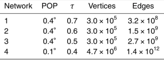
First experiments were performed to construct weighted correlation networks from the 0.4◦ POP grid, having 300 842 grid points. Diff_{erent edge densities (see Table 1)} 5

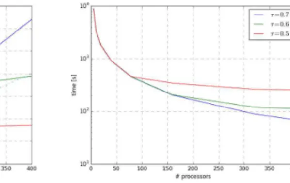
were obtained as a result of applying diff_{erent threshold values}_τ_{for the link definition.} The parallel speedup of the toolbox and the corresponding computational time are plotted in Fig. 3a and b, respectively.

The execution time falls nearly super linearly with the number of processors up to 100. Moreover, the performance becomes strongly super linear forτ >0.5 as the num-10

ber of processors increases. This super linearity is due to a reduction in cache misses at each processor’s cache (note that 20 MB of cache are shared among each 8 cores) as less time series are needed to fit in those shared caches when more cores are im-plied. In a further analysis, we also observed that the reordering of input time series did improve the performance of the toolbox, mainly when the number of processors was 15

less than 100. In the case ofτ=_{0.5, performance drops with larger system sizes. First} thing to remember here is that regardless of the value of the applied τ, the all-to-all correlations are calculated amongst the ring processes. However, the only diff_erence when diff_{erent values of}_τ_{are applied is the amount of data (edges, weights/attributes)} which is sent to the master processor, as they will be more when lower values of τ

20

are applied. That is to say that in such cases, communication overhead hinders the overall performance. The timing for both the parallel reading and the reordering of time series is comparatively constant and pointless compared to the overall execution time, regardless of the number of processors, as shown in Fig. 4.

Similar performance results were obtained for tests using the much larger correlation 25

networks from the 0.1◦ POP grid, resulting in networks of 4.7×106 nodes and edges ranging from 1.5×1010 to 1.4×1012 for thresholds from 0.8 to 0.4, respectively. In summary, it is possible to construct large-scale climate networks in quite reasonable times on modest parallel computing platforms.

(18)

GMDD

8, 319–349, 2015

Par@Graph

H. Ihshaish et al.

Title Page

Tables Figures

◭ ◮

Back Close

Full Screen / Esc

Discussion

P

a

per

|

Discussion

P

a

per

|

Discussion

P

a

per

|

Discussion

P

a

per

|

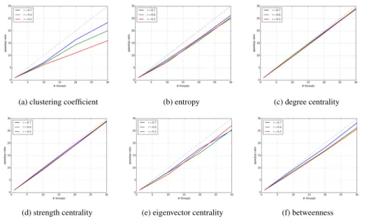
Results of the performance tests to determine the six network properties as dis-cussed in Sect. 2.2 are shown in Fig. 5. As can be seen although there are some dif-ferences in the performance gain in each of the algorithms, a general improvement is achieved by our fine-grained parallel implementation over sequentialigraphalgorithms. In some algorithms, like the clustering coeffi_{cient, parallel performance seems more} 5

sensitive to the density of the network, whereas in others like the degree centrality, per-formance remains intact. However, although an evident perper-formance gain is observed here, one has to remember that the performance of the vast majority of network ana-lyzing algorithms is highly dependent on the topology of the network itself, and thus, further study should be carried out to compare results for diff_{erent types of networks.} 10

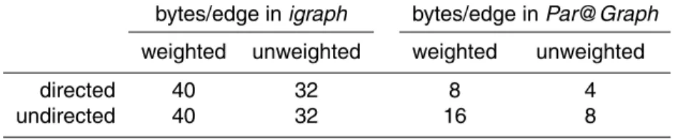
In view of memory requirements, we show in Table 2 a comparison of the needed memory to represent an edge (for diff_{erent types of networks) when using} _igraph_’s data structures with Par@Graph’s adjacency list. Indeed, the presented networks con-structed by our toolbox, as a result of changing the internal data structure, are at least 60 % lighter in size compared to their size in memory when using the original data 15

structures ofigraph.

4.3 Coherence of global sea level

Being able to reconstruct and analyze the large complex networks arising from the POP ocean model, we now shortly demonstrate the novel results one can obtain. One of the important questions in physical oceanography deals with the coherence of the global 20

ocean circulation. In low-resolution (non-eddying) ocean models, the flows appear quite coherent with near steady currents filling the ocean basins. However, as soon as eddies are represented when the spatial resolution is smaller than the internal Rossby radius of deformation, a fast decorrelation is seen in the flow field.

The issue of coherence has for example been tackled by looking at the eigenvalues 25

(19)

GMDD

8, 319–349, 2015

Par@Graph

H. Ihshaish et al.

Title Page

Tables Figures

◭ ◮

Back Close

Full Screen / Esc

Discussion

P

a

per

|

Discussion

P

a

per

|

Discussion

P

a

per

|

Discussion

P

a

per

|

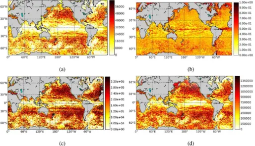
the complex network derived from the SSH data of the 0.4◦POP simulation are shown in Fig. 6a–c. In all cases, a weighted, undirected network was constructed by using the Pearson correlation with zero lag and a threshold valueτ=_0.5.

The precise physical interpretation of these metrics is outside the scope of this pa-per as it requires a background in dynamical oceanography. However, one can ob-5

serve that the subtropical gyres (Dellnitz et al., 2009; Froyland et al., 2014) tend to have a large degree while the regions of the western boundary currents, equator and southern ocean tend to have smaller degree.

In Fig. 6d, the degree field for the network constructed with τ=_{0.4 from the 0.1}◦ POP SSH data is shown. The overall features of the degree field for the 0.1◦ POP data 10

are already found in the degree field for the 0.4◦ POP data, but additional small-scale correlations can be distinguished.

5 Summary and conclusions

Up to now, the data sets (both observational and model based) used to reconstruct and analyze climate networks have been relatively small due to computational lim-15

itations. In this paper we presented the new parallel software toolbox Par@Graph to construct and analyze large-scale complex networks. The software exposes parallelism on distributed-memory computing platforms to enable the construction of massive net-works from a large number of time series based on the calculation of common statisti-cal similarity measures between them. Additionally, Par@Graph is provided with a set 20

of parallel graph algorithms to enable fast calculation of important properties of the generated networks on SMPs. These include those of the betweenness, closeness, eigenvector and degree centralities. Besides the algorithms needed for the calcula-tion of transitivity, connected components, entropy and diameter. Addicalcula-tionally, a parallel implementation of a community detection algorithm based on modularity optimization 25

(Blondel et al., 2008) is provided.

(20)

GMDD

8, 319–349, 2015

Par@Graph

H. Ihshaish et al.

Title Page

Tables Figures

◭ ◮

Back Close

Full Screen / Esc

Discussion

P

a

per

|

Discussion

P

a

per

|

Discussion

P

a

per

|

Discussion

P

a

per

|

The capabilities of Par@Graph were shown by using sea surface height data of a strongly eddying ocean model (POP). The resulting networks had number of nodes ranging from 3.0×105 to 4.7×106, with the number of edges ranging from 3.2×108 to 1.4×1012. The performance of Par@Graph showed excellent parallel speedup in the construction of massive networks, especially when higher thresholds were applied. 5

When lower values of τ were used, communication overhead was seen to decrease the performance. On the other hand, we observed a significant speed gain in the cal-culation of the discussed network characteristics which were obtained by our parallel implementation ofigraph.

With regards to the challenging issue of memory requirements in order to compute 10

such big networks, we showed that the presented toolbox notably optimizes the usage of memory during the reconstruction of large-scale networks by minimizing the accom-panying data redundancy. Additionally, the resulted networks themselves are markedly lighter in size compared to their equivalents inigraphas a result of changing the data structures from indexed edge lists to adjacency lists.

15

The availability of Par@Graph will allow to solve a new set of questions in climate research one of which, the coherence of the ocean circulation at diff_{erent scales, was} shortly discussed in this paper. Apart from higher resolution data sets of one observ-able, it will now also be possible to deal with data sets of several variables and to more effi_{ciently reconstruct and analyze networks of networks (Berezin et al., 2012).} How-20

ever, apart from climate research, Par@Graph will also be very useful for all fields of science where complex and very large-scale networks are applied, and it is hoped that the toolbox will find its way into the complexity science community.

Acknowledgements. The authors would like to acknowledge the support of the LINC project

(no. 289447) funded by EC’s Marie-Curie ITN program (FP7-PEOPLE-2011-ITN). The

compu-25

(21)

GMDD

8, 319–349, 2015

Par@Graph

H. Ihshaish et al.

Title Page

Tables Figures

◭ ◮

Back Close

Full Screen / Esc

Discussion

P

a

per

|

Discussion

P

a

per

|

Discussion

P

a

per

|

Discussion

P

a

per

|

References

Anand, K. and Bianconi, G.: Entropy measures for networks: toward an information theory of complex topologies, Phys. Rev. E, 80, 045102, doi:10.1103/PhysRevE.80.045102, 2009. 326 Berezin, Y., Gozolchiani, A., Guez, O., and Havlin, S.: Stability of climate networks with time,

Scientific Reports, 2, 666, doi:10.1038/srep00666, 2012. 325, 338

5

Blondel, V. D., Guillaume, J.-L., Lambiotte, R., and Lefebvre, E.: Fast unfolding of com-munities in large networks, J. Stat. Mech.-Theory E., 2008, P10008, doi:10.1088/1742-5468/2008/10/P10008, 2008. 337

Bonacich, P.: Factoring and weighting approaches to status scores and clique identification, J. Math. Sociol., 2, 113–120, 1972. 327

10

Brandes, U.: A faster algorithm for betweenness centrality, J. Math. Sociol., 25, 163–177, 2001. 328

Chan, A., Dehne, F., and Taylor, R.: CGMgraph/CGMlib: implementing and testing CGM graph algorithms on PC clusters and shared memory machines, Int. J. High Perform. C., 19, 81–97, doi:10.1177/1094342005051196, 2005. 322

15

Csardi, G. and Nepusz, T.: The igraph software package for complex network research, In-terJournal, Complex Systems, 1695, available at: http://igraph.org (last access: 16 Jan-uary 2015), 2006. 322, 323

Dellnitz, M., Froyland, G., Horenkamp, C., Padberg-Gehle, K., and Sen Gupta, A.: Seasonal variability of the subpolar gyres in the Southern Ocean: a numerical investigation based

20

on transfer operators, Nonlin. Processes Geophys., 16, 655–663, doi:10.5194/npg-16-655-2009, 2009. 336, 337

Donges, J. F., Zou, Y., Marwan, N., and Kurths, J.: Complex networks in climate dynamics, Eur. Phys. J.-Spec. Top., 174, 157–179, 2009a. 320, 325

Donges, J. F., Zou, Y., Marwan, N., and Kurths, J.: The backbone of the climate network,

EPL-25

Europhys. Lett., 87, 48007, doi:10.1209/0295-5075/87/48007, 2009b. 320

Donges, J. F., Schultz, H. C. H., Marwan, N., Zou, Y., and Kurths, J.: Investigating the topology of interacting networks, Eur. Phys. J. B, 84, 635–651, 2011. 320

Dukowicz, J. K. and Smith, R. D.: Implicit free-surface method for the Bryan–Cox–Semtner ocean model, J. Geophys. Res., 99, 7991–8014, 1994. 333

30

Feng, Q. Y. and Dijkstra, H.: Are North Atlantic multidecadal SST anomalies westward propa-gating?, Geophys. Res. Lett., 41, 541–546, 2014. 321, 325

(22)

GMDD

8, 319–349, 2015

Par@Graph

H. Ihshaish et al.

Title Page

Tables Figures

◭ ◮

Back Close

Full Screen / Esc

Discussion

P

a

per

|

Discussion

P

a

per

|

Discussion

P

a

per

|

Discussion

P

a

per

|

Feng, Q. Y., Viebahn, J. P., and Dijkstra, H. A.: Deep ocean early warning signals of an Atlantic MOC collapse, Geophys. Res. Lett., 41, 6009–6015, 2014. 321

Freeman, L. C.: A set of measures of centrality based on betweenness, Sociometry, 40, 35–41, 1977. 327

Froyland, G., Stuart, R. M., and van Sebille, E.: How well-connected is the surface of the

5

global ocean?, Chaos: an Interdisciplinary Journal of Nonlinear Science, 24, 033126, doi:10.1063/1.4892530, 2014. 333, 336, 337

Gozolchiani, A., Yamasaki, K., Gazit, O., and Havlin, S.: Pattern of climate network blinking links follows El Niño events, EPL-Europhys. Lett., 83, 28005, doi:10.1209/0295-5075/83/28005, 2008. 320, 325

10

Gozolchiani, A., Havlin, S., and Yamasaki, K.: Emergence of El Niño as an autonomous com-ponent in the climate network, Phys. Rev. Lett., 107, 1–5, 2011. 320

Gregor, D. and Lumsdaine, A.: The parallel bgl: a generic library for distributed graph com-putations, in: Parallel Object-Oriented Scientific Computing (POOSC), available at: http: //www.osl.iu.edu/publications/prints/2005/Gregor:POOSC:2005.pdf, OSL Indiana University

15

Publications, Indiana, USA, 2005. 322

Hagberg, A. A., Schult, D. A., and Swart, P. J.: Exploring network structure, dynamics, and func-tion using NetworkX, in: SciPy 2008: Proceedings of the 7th Python in Science Conference, edited by: Varoquaux, G., Vaught, T., and Millman, J., 11–15, 2008. 321

Large, W. G. and Yeager, S.: Diurnal to Decadal Global Forcing for Ocean and Sea-Ice

Mod-20

els: the Data Sets and Flux Climatologies, Tech. Rep., National Center for Atmospheric Re-search, Boulder, CO, USA, 2004. 334

Lumsdaine, A., Gregor, D., Hendrickson, B., and Berry, J. W.: Challenges in parallel graph processing, Parallel Processing Letters, 17, 5–20, 2007. 322

Maltrud, M., Bryan, F., and Peacock, S.: Boundary impulse response functions in a century-long

25

eddying global ocean simulation, Environ. Fluid Mech., 10, 275–295, 2010. 334

Mehlhorn, K. and Näher, S.: LEDA: a platform for combinatorial and geometric computing, Commun. ACM, 38, 96–102, 1995. 321

Siek, J., Lee, L.-Q., and Lumsdaine, A.: The Boost Graph Library: User Guide and Reference Manual, Addison-Wesley Longman Publishing Co., Inc., Boston, MA, USA, 2002. 321

30

(23)

GMDD

8, 319–349, 2015

Par@Graph

H. Ihshaish et al.

Title Page

Tables Figures

◭ ◮

Back Close

Full Screen / Esc

Discussion

P

a

per

|

Discussion

P

a

per

|

Discussion

P

a

per

|

Discussion

P

a

per

|

Tirabassi, G. and Masoller, C.: On the eff_{ects of lag-times in networks constructed from} similarities of monthly fluctuations of climate fields, EPL-Europhys. Lett., 102, 59003, doi:10.1209/0295-5075/102/59003, 2013. 325

Tsonis, A. A. and Roebber, P.: The architecture of the climate network, Physica A, 333, 497– 504, 2004. 320, 324

5

Tsonis, A. A. and Swanson, K.: Topology and predictability of El Niño and La Niña networks, Phys. Rev. Lett., 100, 228502, doi:10.1103/PhysRevLett.100.228502, 2008. 320

Tsonis, A. A., Swanson, K., and Kravtsov, S.: A new dynamical mechanism for major climate shifts, Geophys. Res. Lett., 34, 1–5, 2007. 320

Tsonis, A. A., Swanson, K. L., and Wang, G.: On the role of atmospheric teleconnections in

10

climate, J. Climate, 21, 2990–3001, 2008. 320

Tsonis, A. A., Wang, G., Swanson, K. L., Rodrigues, F. A., and Costa, L. D. F.: Community structure and dynamics in climate networks, Clim. Dynam., 37, 933–940, 2010. 320

Tupikina, L., Rehfeld, K., Molkenthin, N., Stolbova, V., Marwan, N., and Kurths, J.: Char-acterizing the evolution of climate networks, Nonlin. Processes Geophys., 21, 705–711,

15

doi:10.5194/npg-21-705-2014, 2014. 325

van der Mheen, M., Dijkstra, H. A., Gozolchiani, A., den Toom, M., Feng, Q., Kurths, J., and Hernandez-Garcia, E.: Interaction network based early warning indicators for the Atlantic MOC collapse, Geophys. Res. Lett., 40, 2714–2719, 2013. 321

Watts, D. J. and Strogatz, S. H.: Collective dynamics of “small-world” networks., Nature, 393,

20

440–442, 1998. 326

Weijer, W., Maltrud, M. E., Hecht, M. W., Dijkstra, H. A., and Kliphuis, M. A.: Response of the Atlantic Ocean circulation to Greenland ice sheet melting in a strongly-eddying ocean model, Geophys. Res. Lett., 39, L09606, doi:10.1029/2012GL051611, 2012. 334, 345

Wyatt, M. G., Kravtsov, S., and Tsonis, A. A.: Atlantic multidecadal oscillation and Northern

25

Hemisphere’s climate variability, Clim. Dynam., 38, 929–949, 2011. 320

Yamasaki, K., Gozolchiani, A., and Havlin, S.: Climate networks around the globe are signifi-cantly aff_{ected by El Niño, Phys. Rev. Lett., 100, 1–4, 2008. 320}

(24)

GMDD

8, 319–349, 2015

Par@Graph

H. Ihshaish et al.

Title Page

Tables Figures

◭ ◮

Back Close

Full Screen / Esc

Discussion

P

a

per

|

Discussion

P

a

per

|

Discussion

P

a

per

|

Discussion

P

a

per

|

Table 1.Diff_{erent threshold values}_τ_{used in the reconstruction of Pearson Correlation networks} from the 0.4 and 0.1◦POP datasets and corresponding number of network vertices and edges.

Network POP τ Vertices Edges

(25)

GMDD

8, 319–349, 2015

Par@Graph

H. Ihshaish et al.

Title Page

Tables Figures

◭ ◮

Back Close

Full Screen / Esc

Discussion

P

a

per

|

Discussion

P

a

per

|

Discussion

P

a

per

|

Discussion

P

a

per

|

Table 2. A single edge’s size in memory when using the indexed edge list used in igraph

compared to its corresponding size when applying Par@Graph. Additionally, a vertex inigraph

is represented by 16 bytes in memory, whereas it needs only 4 bytes in Par@Graph.

bytes/edge inigraph bytes/edge inPar@Graph

weighted unweighted weighted unweighted

directed 40 32 8 4

undirected 40 32 16 8

(26)

GMDD

8, 319–349, 2015

Par@Graph

H. Ihshaish et al.

Title Page

Tables Figures

◭ ◮

Back Close

Full Screen / Esc

Discussion

P

a

per

|

Discussion

P

a

per

|

Discussion

P

a

per

|

Discussion

P

a

per

|

Figure 1.Provided a parallel machine of p processors, p−1 processes are initialized and assigned with equal blocks of time series, each block’s set of time series are correlated, then these blocks are exchanged (p−1)/2 times (half round of the ring) between processes to complete the all-to-all correlations between the whole set of time series. Conversely, p0 is

(27)

GMDD

8, 319–349, 2015

Par@Graph

H. Ihshaish et al.

Title Page

Tables Figures

◭ ◮

Back Close

Full Screen / Esc

Discussion

P

a

per

|

Discussion

P

a

per

|

Discussion

P

a

per

|

Discussion

P

a

per

|

Figure 2.Mean(a)and SD(b)of the daily SSH (units in m) for year 136 of the POP control run as in Weijer et al. (2012).

(28)

GMDD

8, 319–349, 2015

Par@Graph

H. Ihshaish et al.

Title Page

Tables Figures

◭ ◮

Back Close

Full Screen / Esc

Discussion

P

a

per

|

Discussion

P

a

per

|

Discussion

P

a

per

|

Discussion

P

a

per

|

(a) Speedup (b) Execution time corresponding to (a)

(29)

GMDD

8, 319–349, 2015

Par@Graph

H. Ihshaish et al.

Title Page

Tables Figures

◭ ◮

Back Close

Full Screen / Esc

Discussion

P

a

per

|

Discussion

P

a

per

|

Discussion

P

a

per

|

Discussion

P

a

per

|

(a) (b)

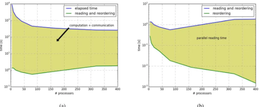
Figure 4.In (a)the overall runtime of the experiment in Fig. 3b (for τ=_{0.5) is shown in the} upper curve and compared to the time for parallel reading and reordering of time series (the lower curve). The shaded area corresponds to real cpu time for the calculation of the corre-lation matrix and the communication between processors. Both times for parallel reading and reordering preprocessing tasks are shown respectively in(b).

(30)

GMDD

8, 319–349, 2015

Par@Graph

H. Ihshaish et al.

Title Page

Tables Figures

◭ ◮

Back Close

Full Screen / Esc

Discussion

P

a

per

|

Discussion

P

a

per

|

Discussion

P

a

per

|

Discussion

P

a

per

|

(a) clustering coefficient (b) entropy (c) degree centrality

(d) strength centrality (e) eigenvector centrality (f) betweenness

(31)

GMDD

8, 319–349, 2015

Par@Graph

H. Ihshaish et al.

Title Page

Tables Figures

◭ ◮

Back Close

Full Screen / Esc

Discussion

P

a

per

|

Discussion

P

a

per

|

Discussion

P

a

per

|

Discussion

P

a

per

|

Figure 6. (a)Degree,(b)clustering and(c)betweenness for the SSH POP data interpolated on the 0.4◦ grid and a threshold ofτ=_0.5._(d) _{Degree field for the 0.1}◦ _{grid and a threshold} τ=_{0.4; here the reconstructed network has 4.7}_×₁₀6_{nodes and 1.4}_×₁₀12_edges.