©2014 Science Publication
doi:10.3844/ajassp.2014.789.810 Published Online 11 (5) 2014 (http://www.thescipub.com/ajas.toc)
Corresponding Author: Hiram Ponce, Graduate School of Engineering, Tecnológico de Monterrey, Campus Ciudad de México, 14380, Mexico City, Mexico
A NOVEL ARTIFICIAL HYDROCARBON NETWORKS
BASED SPACE VECTOR PULSE WIDTH MODULATION
CONTROLLER FOR INDUCTION MOTORS
Hiram Ponce, Luis Ibarra, Pedro Ponce and Arturo Molina
Graduate School of Engineering, Tecnológico de Monterrey, Campus Ciudad de México, 14380, Mexico City, Mexico
Received 2013-12-22; Revised 2014-02-04; Accepted 2014-02-26
ABSTRACT
Most of machine-operated industrial processes implement electric machinery as their work sources, implying the necessary improvement of control techniques and power electronics drivers. Many years have passed since the control conflicts related to induction motors have been overcome through torque-flux control techniques so their advantages over direct current motors have made them to be the most common electric actuator found behind industrial automation. In fact, induction motors can be easily operated using a Direct Torque Control (DTC). Since, it is based on a hysteresis control of the torque and flux errors, its performance is characterized by a quick reaching of the set point, but also a high ripple on both torque and flux. In order to enhance that technique, this study introduces a novel hybrid fuzzy controller with artificial hydrocarbon networks (FMC) that is used in a Space Vector Pulse Width Modulation (SVPWM) technique, so-called FMC-SVPWM-DTC. In fact, this study describes the proposal and its design method. Experimental results over a velocity-torque cascade topology proved that the proposed FMC-SVPWM-DTC responses highly effective almost suppressing rippling in torque and flux. It also performed a faster speed response than in a conventional DTC. In that sense, the proposed FMC-SVPWM-DTC can be used an alternative approach for controlling induction motors.
Keywords: Direct Torque Control, Spatial Vector PWM, Artificial Hydrocarbon Networks
1. INTRODUCTION
Since the Direct Torque Control (DTC) was proposed in the 1980’s by Takahashi and Noguchi (1986) it has been widely used as it offers a direct and simple way to control the stator’s flux and electromagnetic torque of Alternating Current (AC) machines, using only phase voltage and current sensors to estimate the pertinent variables. As it is based on hysterical control of the torque and flux errors, its performance is characterized by a quick reaching of the set point but also a high ripple on both magnitudes.
Having such a high ripple in torque and flux is due to the pulsed characteristic of the phase voltages delivered by a Voltage Source Inverter (VSI) without modulation, thus applying discontinuous phase
currents highly contaminated by harmonics and damaging the machine. So reducing the ripple in torque and flux becomes paramount for an improved harmless direct control technique.
In order to enhance the way the voltage is delivered to the machine, a modulation technique is placed instead the hysteresis bands, calculating the VSI combination needed through Proportional-Integral (PI) controllers and executing it with a Space Vector Pulse Width Modulation (SVPWM) technique. This topology provides great performance as shown in literature (Wahab and Sanusi, 2008) and is commonly named for short as SVPWM-DTC.
proposes to hold the DTC almost unchanged but improves the way the hysteresis band is calculated as in (Sanila, 2012) or includes a zero voltage state to modulate the time each VSI combination is applied like in (Ab Aziz and Ab Rahman, 2010). Different works pretend to improve the control applied so they add dynamical adaptation capabilities to PI controllers through inferences over torque error and current’s magnitude (Wang et al., 2011; Sheng-Wei et al., 2010), or uses fuzzy control instead of PI controllers like in (Zheng et al., 2011; Abdalla et al., 2010; Zaimeddine and Berkouk, 2007; Azcue et al., 2011; Naik and Singh, 2012).
Truth is SVPWM-DTC has become a foundation in automatic control of electric machines because its good results and simplicity and its capability to embed new and different techniques to present remarkable improvements in direct torque and cascade speed control. Some application examples of the technique itself or with little variations can be found in (Singh et al., 2012; Wahab and Sanusi, 2008; Che and Qu, 2011).
In the present work, a novel hybrid fuzzy controller which implements Artificial Hydrocarbon Networks (AHN) as a mean of defuzzification is presented as a replacement of PI controllers for voltage vector selection to be sent to the SVPWM modulator achieving good results. Thus, the study is organized as follows: Section 2 presents an overview of the conventional DTC using a space vector pulse width modulation technique, section 3 briefly reviews artificial hydrocarbon networks, Section 4 presents the proposed fuzzy controller using AHN and its design method. Then, section 5 describes the results of the proposed SVPWM with the fuzzy controller using AHN and discusses the proposed controller in comparison with a conventional DTC controller. Finally, section 6 concludes the study.
1.1. Overview of the Conventional DTC Using a
SVPWM Technique
This section presents a review of the conventional Direct Torque Control (DTC) firstly proposed in (Takahashi and Noguchi, 1986) using a Space Vector Pulse Width Modulation (SVPWM), also named SVPWM-DTC, as shown in Fig. 1.
1.2. Voltage Source Inverter and the d-q
Transformation
Three-phase AC machines has replaced Direct Current (DC) ones and have quickly and widely
spread among diverse applications of electric drives due to their advantages like improvement of energy efficiency and low maintenance requirements, nevertheless, their speed is related with (but not limited to) the AC fed frequency so its control can be seen as complicated when compared to that of DC motors which can be directly modified by means of changing the input voltage. This detail made its use to be restricted to constant speed applications until a way to vary its input frequency was found, mostly thanks to developments in switching power electronics uses.
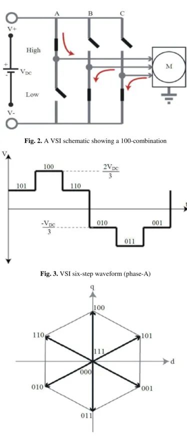
Generally speaking, a power inverter is a device which can convert from a DC input to an AC output through the commutation of two semiconductors with one of their terminals connected to the same output node and the other to the positive and negative terminals of the DC input respectively. In order to drive three-phase electric machines, three pairs of electronic devices are needed (one per phase) to connect cyclically each of the machine’s terminals to a varying voltage. If all semiconductors were schematically represented as switches, a VSI connected to a motor would look like as
Fig. 2 (Singh et al., 2012).
It is easy to see that the whole three-phase VSI will have eight possible combinations from which six can drive current to the motor while the remaining two connects its three terminals to the same node; an easy way to address these combinations is by three individual numbers which represent the state of each inverter’s leg: If the number is 1, then the high semiconductor is closed and the low opened and the related phase is connected with the positive DC terminal, if it is 0 the low semiconductor is closed and the high one opened, so the related phase is connected with the negative DC terminal (Fig. 2 shows a (100) combination). Notice that both transistors of a particular leg can never be closed together as the DC source would become short-circuited.
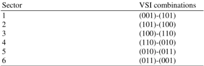
If the semiconductors of the VSI are switched with a particular sequence and they energize the motor’s windings properly, it will rotate. The proper sequence chosen to power the machine can be executed at different rates, thus, modifying the frequency at which it is fed and solving the speed control conflict. Using the VSI combinations themselves, an emulation of a sinusoidal wave can be delivered to the motor as shown in Fig. 3, the waveform generated in this way is called six-step as it is based on those six VSI combinations which can deliver power to the machine.
sequence applied, the consequent current and the generated stator’s magnetic flux are some of those variables. If the motor is seen transversally from its front plate, the electric contribution of all three phases can be seen as a two-dimensioned vector, in this way, a transformation is used to map from a three-dimensioned value to a planar representation, this mapping is called Park transformation Equation 1:
A q
B d
C
1 1 X
1
X 2 2 2
= X
3 3 3
X 0
-X
2 2
− −
(1)
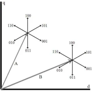
If the VSI combinations are mapped through (1) and can be represented in a plane denominated d-q frame, shown in Fig. 4 (Takahashi and Noguchi, 1986). From this representation it is evident that the machine phases are electrically distributed radially on the stator separated equally by 120° as the
combinations which applies voltage only to one phase are A-100, B-010 and C-001 (Notice combinations 111 and 000 are mapped as 0 vectors). This representation is consistent with the sinusoidal emulation shown before in Fig. 3 considering the rotation of the vector representation to be Counterclockwise (CCW).
If VSI combinations are delivered to the motor in the way described above the frequency of the emulated sinusoidal signal can be modified as desired, nevertheless, its magnitude cannot. A different problem arises considering the applied voltage is delivered in squared steps so the current harmonics on the motor’s phases would be high. Both described problems are due to the un-modulated nature of the VSI combinations (Wahab and Sanusi, 2008), SVPWM is a modulation technique that allows a VSI to deliver an arbitrary voltage vector by combining VSI voltage and zero vectors in regulated periods of time (Sanila, 2012).
Fig. 2. A VSI schematic showing a 100-combination
Fig. 3. VSI six-step waveform (phase-A)
Fig. 5. Comparison of a symmetric PWM Table 1. Sector distribution of VSI representation
Sector VSI combinations
1 (001)-(101)
2 (101)-(100)
3 (100)-(110)
4 (110)-(010)
5 (010)-(011)
6 (011)-(001)
1.3. SVPWM Technique
A conventional way to emulate the phase shifted sinusoidal waves is to generate any desired vector (within the VSI representation) through the combination of VSI ones (Sanila, 2012), this is, to hold (101) for a certain time and (100) for another, making possible to represent any vector between 30-90°, moreover, if a different voltage magnitude is wanted, (000) and (111) vectors can also be used to reduce it. So the total PWM period is formed by three different ones TPWM = T0+T1+T2, where the subscript represent
the VSI combination involved and 0 represents (000) and (111) combinations.
For the combinations proposed above, A-leg would remain high for the entire PWM period unless a reduced voltage vector magnitude is desired, in that case, low states should be added to it. On the other hand the opposite should be done for B-leg that is normally low for the entire operation. After analyzing C-leg, it would have a high state for a time T1 and a low one for T2, so reducing
vector’s magnitude could be done by changing some high states of T1 with low ones and some low states from T2
with high ones. So T0 should be divided in two equal
parts, one for each zero voltage VSI combination. If the phase outputs were to be delivered with a traditional PWM, all legs of the VSI would change
simultaneously at the beginning of TPWM, in order to avoid this undesired effect, a symmetrical PWM is used like the one shown in Fig. 5, a symmetrical perspective would also make clearer the addition of zero voltage vectors through T0 like shown in Fig. 6.
Figure 6 shows a generalized commutation scheme of SVPWM technique (Singh et al., 2012), notice that A-leg is normally high, B-A-leg is a combination of high and low states and C-leg is normally low. This ordering would be appropriate for an arbitrary vector defined between (110) and (100) combinations, so the state assigned to each phase for a particular time period depends on the actual position of the desired output vector. The VSI vector representation could be divided in sectors as in Table 1.
Depending on the sector the desired vector is, the states will be assigned to the different phases, nevertheless, the times can be calculated in the same way for all the sectors like in (2) depending only on the angle α defined inside each sector [0-60º] with reference to the lower closest VSI vector and on V which is the desired vector magnitude Equation 2:
(
)
(
)
o
1 PWM
2 PWM
0 PWM 1 2
T = 2T V cos α+ 30
T = 2T V cosα
T = T - T + T
(2)
Each sector is then limited by an Upper Boundary (UB) and a lower one (LB), (001) is the LB of the first sector, (101) is the LB of the second one and so on. Depending on the sector de desired vector is, T1 will be
assigned to the LB and T2 to the UB if the sector number
Fig. 6. SVPWM commutation scheme
1.4. Conventional Direct Torque Control
Direct torque control enables the direct control of torque and stator’s flux magnitudes with quick settling times and improved computational performance, as it is based in hysteresis bands comparison technique and a constant-table that assigns a VSI vector depending on the torque and flux errors conditions (Takahashi and Noguchi, 1986). This technique strictly needs two current sensors to work properly and the magnitude of stator’s resistance, making its application easy and straightforward to follow.
Park transformation (1) can be used for voltages and currents to map both magnitudes on the d-q frame, as shown before. The d-q representation is congruent with the electrical distribution of the motor so the stator’s flux can be calculated as (3), integrating the voltage present at the inductive part of the phase winding. On the other hand, torque can be calculated as (4); where, its magnitude and direction are subjected to the phase-shift of the previously calculated components Equation 3 and 4:
(
)
d,q Vd,q Rid,q dt
Ψ =
∫
− (3)q d d q
T= Ψ i − Ψ i (4)
If a voltage vector is applied to the machine, e.g., the VSI combination (100), the magnetic flux of the motor will increase along the q axis direction due to its physical phases’ distribution, this implies that the stator flux vector’s angle and magnitude will be modified congruently with the angle and magnitude of the applied voltage vector, so a way to control the stator’s flux is revealed. Torque control can be achieved in a similar way considering that it proceeds from the
separation of stator and rotor’s fluxes, so assuming rotor’s flux will follow the stator’s one, using a voltage vector which takes the stator’s flux vector further in the desired direction would make the torque to increase (Takahashi and Noguchi, 1986).
Consider two different stator’s flux vectors A and B shown in Fig. 7, if the torque is assumed to be positive in the CCW direction, then applying a (110) combination would highly augment the torque and slightly increase the flux magnitude for vector A while it would improve the torque but decrease the flux for vector B. This means that the application of the VSI voltage vectors depends on the flux vector’s actual position, making necessary to define it in terms of sectors as shown in Table 2.
So the voltage vectors to be sent to the machine depend on both the torque and the flux errors and the sector in which the actual stator’s flux vector is. A single hysteresis band processes the flux magnitude error so it needs a set point and a band gap, which it will establish the positive and negative limits for the flux error so a decision about increasing or decreasing it could be taken. Torque is processed through a double hysteresis band as long as its set point can be positive or negative (a band gap must also be defined), if positive, the set point will work as the high limit for a single hysteresis band and if negative, it will be taken as the lower limit of another single band as shown in Fig. 8.
Fig. 7. Flux and VSI-voltage vectors representations
Fig. 8. Double hysteresis band representation for torque control Table 2. Sector definition for a DTC application
Sector Boundaries (°)
1 0-60
2 60-120
3 120-180
4 180-240
5 240-300
6 300-0
Based on the above information, the VSI voltage vectors can be now chosen so that the stator’s flux and torque characteristics can be modified as shown in Table 3. The vector selection will be made after acquiring or estimating voltage and current variables and processing the necessary operations to compute (3) and (4). This implies the VSI vector will be able to change after a certain amount of time in equal intervals. Based on
Table 3 and considering the described hysteresis flux band, a diagram showing the execution of the DTC algorithm over the flux vector of a certain motor is presented in Fig. 9, while a block diagram of the whole technique is shown in Fig. 10.
Using the traditional DTC technique shown in Fig. 10 would yield to some known problems related with current harmonics (Sanila, 2012) and torque and flux ripples. There is another common issue with torque stability when the flux vector is close to the sector limits; if the VSI vectors are applied as indicated in Table 3, the flux vector behavior will be different depending on which zone inside every sector it is, besides this can be noticed from Fig. 9 a closer view is offered in Fig. 11
where the effect of being close to the sector change becomes evident if taking the same amount of time periods around the sector limit (marked as a, b and c). Notice that the contribution to torque for periods a and c is much higher than the one of period b. The effect disparity of a certain vector’s position, the evident ripple due to the hysteresis bands, the execution time of the algorithm and the exclusive use of six-step combinations are the reasons why the DTC, besides being a quick and easy direct control technique, delivers a poor performance for most of the applications.
If a modulation technique is used to generate the proper voltage vector based on a desired angle and magnitude, then the problems mentioned above can be eliminated (Wahab and Sanusi, 2008), nevertheless if no hysteresis bands are used, more complex control topologies are needed and the overall technique becomes complicated and more computational applicant.
1.5. SVPWM-DTC
The SVPWM-DTC topology differs from the conventional DTC in two main aspects: It uses PI controllers instead of hysteresis bands and a SVPWM modulation technique to replace the table with the predefined VSI voltage vectors. The block diagram shown in Fig. 1 shows those changes compared to that on Fig. 9. In this controller, it is important to know the angle of the stator’s flux vector instead of the sector, so the voltage vector sent to the motor compensates torque and flux magnitude errors effectively.
Table 3. VSI voltage vector selection table
S1 S2 S3 S4 S5 S6
↑F ↑T (100) (110) (010) (011) (001) (101) - T (000) (111) (000) (111) (000) (111)
↓T (001) (101) (100) (110) (010) (011)
↓F ↑T (110) (010) (011) (001) (101) (100) - T (111) (000) (111) (000) (111) (000)
↓T (011) (001) (101) (100) (110) (010) Symbols mean: ↑ increase, ↓ decrease and – hold (positive torque is assumed to be CCW)
Fig. 9. DTC operation over stator’s flux vector
Fig. 10. Block diagram of the conventional DTC
Fig. 11. Sector change known issues in torque degeneration
Fig. 12. Normal operation of the SVPWM-DTC
The normal SVPWM-DTC operation is shown in Fig. 12. Notice how the response is sector independent and the overshooting can be regulated to be lower than the one generated by the hysteresis band, as the torque magnitude is controlled in a similar way. The problem about torque degeneration on sector limits is also corrected.
1.6. Review of Artificial Hydrocarbon Networks
Ponce and Ponce (2011) and then it describes the particular Artificial Hydrocarbon Networks (AHN) algorithm derived from AON and inspired on chemical hydrocarbon compounds.
1.7. Artificial Organic Networks
Chemical organic compounds are the most stable ones in nature. Its inner structure reveals important information that can be used as inspiration. For example, molecules can be seen as units of packaging information; that combined in specific arrangements can determine a nonlinear interaction of data. In addition, molecules can be related to encapsulation and potential inheritance of information, e.g., functional groups. Also, these chemical organic compounds are stable due to the strength of carbon-carbon bonds and the hierarchical strategy of organization. For example, at first basic molecules are formed in order to minimize energy in the structure. If atoms in molecules can accept more bonding atoms, then complex molecules are formed. At last, if these complex molecules cannot perform a desired action, mixtures of them can be made. Thus artificial organic networks take advantage of this knowledge, inspiring a class of computational algorithms that can infer and classify information based on stability and chemical rules that allow formation of molecules (Ponce et al., 2014). In that sense, AON define four components and two basic interactions among them, as follows (Ponce et al., 2014; Ponce and Ponce, 2012).
On one hand, the four components are: Atoms, molecules, compounds and mixtures. Atoms are the basic units with structure. No information is actually stored. The number of degrees of freedom can differentiate two atoms. If they have equal number of atoms, they are similar atoms and different atoms otherwise. In terminology, the degree of freedom is the number of valence electrons in an atom that allow it linking among others. Molecules are made of two or more atoms and represent the basic unit of information with structural and behavioral properties. Structurally, they conform the basis of an organized structure while behaviorally they can contain nonlinear information. Compounds are a special type of molecules made of two or more basic molecules, arising complex molecules. Notice that compounds in AON is slightly different from a chemical point of view. Lastly, mixtures are linear combinations of molecules and/or compounds forming a basis of
molecules with weights so-called stoichiometric coefficients. On the other hand, the two interactions among components are covalent bonds and chemical balance interaction. Covalent bonds are relationships between two atoms and are of two types. Polar covalent bonds refer to the interaction of two similar atoms, while nonpolar covalent bonds refer to the interaction of two different atoms. In addition, chemical balance interaction refers to find the proper values of stoichiometric coefficients in mixtures in order to satisfy constrains of artificial organic networks.
1.8. Artificial Hydrocarbon Networks
Artificial Hydrocarbon Networks (AHN) is a supervised learning algorithm based on artificial organic networks that implements notions of chemical hydrocarbon compounds in order to infer and classify data from a given unknown system (Ponce et al., 2014; Ponce and Ponce, 2012). Also, artificial hydrocarbon networks define proper components and interactions under the AON technique. As a learning algorithm, AHN proposes two steps: Training and reasoning procedures.
1.9. Components and Interactions
Artificial hydrocarbon networks only considers two types of atoms: Hydrogen atoms H each one with one degree of freedom and carbon atoms C each one with up to four degrees of freedom (Ponce et al., 2014; Ponce and Ponce, 2012).
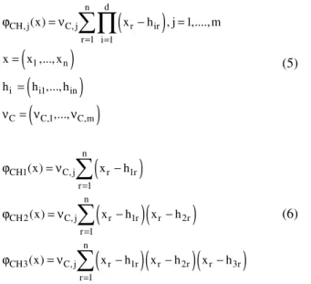
The basic unit of information is called CH-molecule and it is shown in Fig. 13. These kinds of molecules are structurally made of hydrogen and carbon atoms following the so-called octet rule (Ponce and Ponce, 2012). For instance, let Mi be the structure of a
molecule and φi be the behavior of that molecule.
Then, a CHmolecule MCH has a molecular behavior
φCH defined as (5); where, hi is a complex vector
called hydrogen value, vC is a real vector called
(
)
(
)
(
)
(
)
d nCH, j C, j r ir r 1 i 1
1 n
i i1 in C C,1 C,m
(x) x h , j 1,...., m
x x ,..., x
h h ,..., h
,..., = =
ϕ = ν − =
=
=
ν = ν ν
∑
∏
(5)(
)
(
)(
)
(
)(
)(
)
nCH1 C, j r 1r r 1
n
CH2 C, j r 1r r 2r r 1
n
CH3 C, j r 1r r 2r r 3r r 1
(x) x h
(x) x h x h
(x) x h x h x h
=
=
=
ϕ = ν −
ϕ = ν − −
ϕ = ν − − −
∑
∑
∑
(6)
Furthermore, let Ci be a compound formed with a set
of p CH-primitive molecules. Then, its behavior Ψi can
be expressed like (7); where, φj are the behaviors of the
CH-primitive molecules and π is the behavior of nonpolar covalent bonds that relates molecules between them (Ponce et al., 2014; Ponce et al., 2013a) Equation 7:
(
)
i 1,..., j,..., p, x ,i 1,..., m
ψ = π ϕ ϕ ϕ = (7)
Finally, a mixture of molecules (or compounds) S is expressed as a linear combination of them, like (8); where, αi is a set of stoichiometric coefficients representing the ratio of molecules in the mixture (Ponce et al., 2014) Equation 8:
(
)
p j i, j i, j
i 1 i i,1 i,m
S (x) (x), j 1,...m
,..., =
= α ψ =
α = α α
∑
(8)
To this end, artificial hydrocarbon networks are mixtures of molecules, as shown in Fig. 14. In order to create these mixtures of molecules that learn from observed data, a training procedure, the AHN-algorithm, was depicted in (Ponce et al., 2014).
1.10. The AHN-Algorithm
Consider a set of observed data in the form of inputoutput pairs Σ = (x,y), called the training set.
Fig. 13. The basic unit of an artificial hydrocarbon network
Fig. 14. A simple artificial hydrocarbon network
Then, an artificial hydrocarbon network has to learn this set Σ using the training procedure summarized in Algorithm 1 (AHN-algorithm); which it receives the training set Σ, the maximum number of CH-primitive molecules p and the number of compounds c.At last, the AHN-algorithm outputs the structure of the mixture, the set of hydrogen values and the set of stoichiometric coefficients (Ponce et al., 2014): • Initialize a compound
• Build the structure of the compound • Optimize and train the compound
• If the enthalpy rule failed, go to (Abdalla et al., 2010) • If the tolerance condition failed
• Recalculate the residue and go to (Ab Aziz and Ab Rahman, 2010)
• Create a mixture of compounds • Return the mixture
Roughly speaking, the AHN-algorithm approximates the training set by creating and connecting CH-primitive molecules. At the beginning, two molecules are present. However, if the training set is not well approximated, then more CH-primitive molecules are added in a string of molecules (i.e., a compound), until an enthalpy-based rule condition is reached (Ponce et al., 2014). This rule measures the energy of both the training set and the actual compound and compares them in a ratio like (9); where, Hf is the enthalpy (energy) of a set f and f(xi) is the i-th
output value of f. The rule is reached when m is less or equal than 1 Equation 9:
( )
2f i
C i
H
m , H f x
H ∑ ∆
= ∆ =
∆
∑
(9)While a compound is forming, the set of hydrogen values and carbon values of each CH-primitive molecule are calculated using a Least Square Estimates (LSE) method that compares a subset of the training set Σ with one molecular behavior. Actually, p subsets of the training set are calculated using a modified covalent bond based algorithm originally reported in (Ponce et al., 2013a).
For instance, consider an intermolecular distance that defines the length between the positions of two molecules. Actually, the algorithm randomly initializes the positions of molecules and iteratively updates the set of intermolecular distances to define the best positions of molecules in the input domain space using the update rule (10); where, r represents the intermolecular distance between two molecules M1 and M2, Ej,1 and Ej,2 are the
square errors of each molecule and 0<η<1 is the step size or the learning rate Equation 10:
j j j,1 j,2 1 j m
r = − ηr (E −E ) r=(r ,..., r ,..., r ) (10)
At each iteration, the intermolecular distances are updated; and fixing the first molecule of the compound to a reference in the input domain, e.g., L0, it is possible
to determine the positions of all the molecules in that compound, using (11); where, Li represents the position of the i-th molecule and ri-1,I is the intermolecular
distance between molecules Mi-1 and Mi Equation 11:
i i 1 i 1,i
L =L− +r− (11)
To this end, a compound approximates the training set. In order to maximize the accuracy of the approximation, more compounds can be added by using the same methodology as before, until a tolerance-based condition
ε>0 is reached, defined as (12); where, Ri is calculated as
(13) after (12) is evaluated, y represents the output value of the training set and Ci is the i-th compound (Ponce and
Ponce, 2012; Ponce et al., 2014) Equation 12 and 13:
i i 1
R −C ≤ ε, R =y (12)
i i 1 i 0
R =R− −C , R =y (13)
More detailed information about the AHN-algorithm be found in (Ponce et al., 2014).
1.11. Reasoning Step
Once the training is done, an artificial hydrocarbon network can be used for reasoning. In that sense, consider an input value x0. The artificial hydrocarbon network
AHN can be evaluated in x0 using (14) in order to find an
inferred output value y0; where, S is the behavior of the
artificial hydrocarbon network, H is the set of all hydrogen atoms in the structure, Λ is the set of stoichiometric coefficients, R is the set of all intermolecular distances between molecules and V are the set of all carbon values (Ponce et al., 2014) Equation 14:
0 0
y =S(x H, , R, V)Λ (14)
1.12. Description of the Proposed
Fuzzy-Molecular Controller
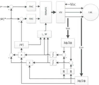
This section introduces and describes a novel SVPWM strategy for a DTC controller based on a hybrid fuzzy inference system using artificial hydrocarbon networks, named Fuzzy-Molecular Controller (FMC for short). In a nutshell, the proposed SVPWM-DTC using fuzzy-molecular controllers replaces the PI controllers from the conventional SVPWM-DTC topology of Fig. 1, with two FMC that determine the optimal voltage vector (separated in magnitude and angle) that has to be sent to the SVPWM, resulting in the FMC-SVPWM-DTC topology shown in Fig. 15.
In order to understand the proposed topology, the fuzzy-molecular controller is introduced below, as well as, the design method of this FMC for implementing the resultant FMC-SVPWM-DTC topology.
1.13. Fuzzy-Molecular Controller
Fig. 15. Block diagram of the proposed FMC-SVPWM-DTC
The block diagram of the fuzzy-molecular controller is shown in Fig. 16. As noted, FMC has three steps:
fuzzification, fuzzy inference engine and defuzzification and it also assumes a knowledge base.
1.14. Fuzzification Step
This is the first step of the FMC that receives a set of
crisp inputs (e.g., an error signal) and maps it to a set of fuzzy values, each one in the range [0,1]; which it represents the degree of membership that an input has over a fuzzy set. This mapping occurs using a fuzzy set Ai and its corresponding membership function Ai like (15); where, x represents a crisp input Equation 15:
[ ]
Ai(x) : x 0,1µ ֏ (15)
For instance, an input variable can be partitioned into m different fuzzy sets {Ai}, such as: “very negative” or
“positive”. Common membership functions can be found in literature so as in (Ponce et al., 2013b).
1.15. Fuzzy Inference Engine Step
The second step in the FMC is the fuzzy inference engine in which a set of fuzzy rules Rt expressed as (16) are
evaluated so that an inference process is done using the set of fuzzy values already calculated in the fuzzification step, also known as the antecedents of the fuzzy rules. Notice that (16) associates the behavior of a CH-primitive molecule Mj
as the consequent value yt Equation 16:
t 1 1 k k t j
R : if x is A and....andx is A , then y is M (16)
Different techniques can be used for evaluating the antecedents, like the min-operation (Ponce et al., 2013b). In that sense, the evaluation of the consequent value yt can be computed using the fuzzy rule of the form as (16) and the min-operation, as expressed in (17); where, φj
represents the behavior of molecule Mj Equation 17:
{
}
t j A1 1 Ak k
y = ϕ (min µ (x ),...,µ (x ) ) (17)
1.16. Defuzzification Step
The last step in the fuzzy-molecular controller is the defuzzification step. It calculates a crisp output value y, e.g., the correction signal. Considering n fuzzy rules defined on the FMC, the i-th value of the antecedents (i.e.,
the min-operation) can be expressed as (18). Then, the output value y can be computed with the center of gravity method as shown in (19); where yi is the i-th consequent value calculated using (17) Equation 18 and 19:
{
}
i(x ,..., x )1 k min A1(x ),...,1 Ak(x )k
µ = µ µ (18)
n
i 1 k i
i 1 n
i 1 k
i 1
(x ,..., x ) y
y
(x ,..., x )
= =
µ =
µ
∑
∑
i
Fig. 16. Block diagram of the fuzzy-molecular controller
In general, the fuzzy-molecular controller restricts the usage of a single artificial hydrocarbon compound made of a set of s different CH-primitive molecules Mj for all j
= 1, …, s. As proved in (Ponce et al., 2013b), using a fuzzy inference system with artificial hydrocarbon networks allows to fuzzy partition the output domain in linguistic-molecular units like: “Positive”, “zero”, “negative”. Also, this hybrid approach allows dealing with noisy and uncertain data, for example, perturbations in SVPWM-DTC controller.
1.17. Knowledge Base
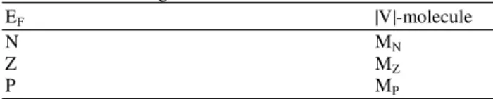
The knowledge base collects and summarizes the fuzzy rules used in the FMC. It is a table with a set of k columns representing the crisp inputs in the antecedents of the rules and a column representing the molecular unit of the consequent value. An example of a knowledge base is shown in Table 4.
1.18. Design of the FMC for SVPWM-DTC
As shown in Fig. 15, the proposed FMC-SVPWMDTC is based on two fuzzy-molecular controllers, one associated to the torque and the other to the stator’s flux. In particular, the proposal considers to regulate the magnitude of the voltage vector |V| using the error EF between the
magnitude of the stator’s flux set point |F|* and the actual magnitude of the stator’s flux |F| and to regulate the angle of the voltage vector θV using both the error ET between
the torque set point T* and the actual torque T and the integral in error I(ET), lastly adding this quantity to the
actual angle of the stator’s flux θF. These fuzzy-molecular
controllers are explained below.
1.19. FMC of Magnitude of the Voltage Vector
Consider the regulation of stator’s flux in the way of the six-step as depicted in Fig. 7 and 9. As said previously in section 2, the idea is to control the stator’s flux by modifying the magnitude of the voltage vector, like the SVPWM-DTC shown in Fig. 12.
Table 4. Proposed knowledge base for the FMC of magnitude of the voltage vector
EF |V|-molecule
N MN
Z MZ
P MP
It is easy to check that the error EF between the
magnitude of the stator’s flux set point |F|* and the actual magnitude of the stator’s flux |F|, is proportional to the magnitude of the voltage vector |V|. For example, if EF is
positive, |V| has to increase; while EF is negative, |V| has to
decrease. In that sense, a FMC for the magnitude of the voltage vector proposes to enclose the above description into the fuzzy knowledge base depicted in Table 4. For instance, EF is fuzzy partitioned into three fuzzy sets:
“Negative” (N), “Zero” (Z) and “Positive” (P). Also, the output |V| is fuzzy represented into three different linguistic-molecular units: “Negative” (MN), “zero” (MZ) and
“positive” (MP). Notice that more than three fuzzy partitions
in the input and output domains might be done.
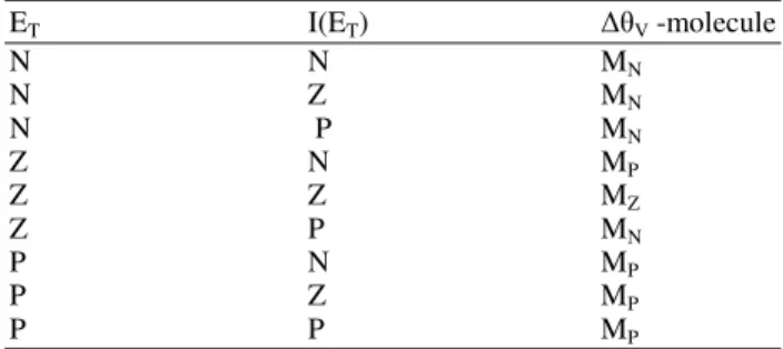
1.20. FMC of Angle of the Voltage Vector
On the other hand, doing a similar analysis as described in section 2, the angle of the voltage vector θV can be also modified using the error ET between the
torque set point T* and the actual torque T and adding this value to the actual angle of the stator’s flux θF. It
means that, if ET increases, then the change of the angle of the voltage vector θV will increase, while if
ET decreases, then θV will decrease. Table 5
summarizes the above observations. Normally, the actual torque T remains behind T*, arising large steady-state error values in ET. Then, other strategies like using the integral of ET, I(ET) for short, can be taken into account when designing controllers. In that sense, the proposed FMC for the angle of the voltage vector proposes to use both ET and I(ET) like the fuzzy
Table 5. Proposed knowledge base for the FMC of angle of the voltage vector
ET I(ET) θV -molecule
N N MN
N Z MN
N P MN
Z N MP
Z Z MZ
Z P MN
P N MP
P Z MP
P P MP
For instance, both input values ET and I(ET) are
fuzzy partitioned into three fuzzy sets: “Negative” (N), “Zero” (Z) and “Positive” (P). Also, the output θV is
fuzzy represented into three different linguistic-molecular units: “Negative” (MN), “zero” (MZ) and
“positive” (MP). Again, both inputs and output might
have more than three fuzzy partitions. Finally, the updated angle θV can be computed using (20):
v v F
θ = ∆θ + θ
2. RESULTS
This section introduces the results of the proposed FMC-SVPWM-DTC over a speed-torque cascade topology. It also compares the proposal with a conventional DTC strategy in order to evaluate its performance.
2.1. Description of the Experiment
Torque itself is not a variable whose control can be effectively used in industrial applications, besides there are particular needs of variable torque controllers which are most of the times inside another control topology like speed regulation or optimal control. This means that torque control is usually found as the center part of cascade controllers, i.e., inside speed loops.
To evaluate the performance of the proposed FMCSVPWM- DTC, a speed-torque cascade controller was implemented, as shown in Fig. 17, where the proposed FMC-SVPWM-DTC conforms the inner control loop and another PI controller offers a torque set point from the evaluation of the speed error. In this application, the stator’s flux magnitude is set to be constant for the whole operation.
In particular, the speed-torque cascade topology as well as the performance of both the proposed FMCSVPWM- DTC and the conventional DTC topologies, was implemented in Simulink®. The parameters of the
induction motor used in the experiment are summarized in
Table 6. A constant load-torque of 5 Nm with a constant stator’s flux magnitude set point of 1.5 Wb and a constant velocity set point of 50rad/s were considered.
For comparison purposes, a conventional DTC technique was implemented using the topology shown in
Fig. 1. In that sense, the hysteresis band associated to the stator’s flux is |0.01| ≤ EF and the hysteresis band associated
to the torque is |0.5|≤ET. Additionally, for both the proposed
FMC-SVPWM-DTC and the conventional DTC based topologies, the PI controller associated to the speed controller has gains KP = 15 and KI = 1.
2.2. Performance of the Conventional DTC
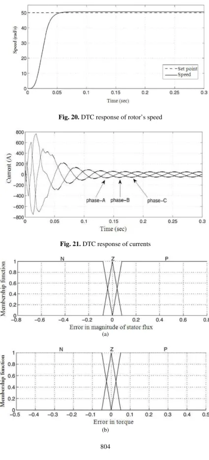
The conventional DTC controller was implemented and run, in order to regulate the speed of the rotor in the induction motor described in Table 6. In that sense, Fig. 18 reports the response of the stator’s flux in terms of its magnitude, Fig. 19 shows the response of the torque,
Fig. 20 shows the response of the rotor’s speed and the three-phase currents of the AC motor are shown in Fig. 21. As noted, the stator’s flux rippled over the set point but tiny attenuations (white spaces) are observed. In torque, the transient and steady states are well performed. In terms of speed, it reached the set point in a settling time of 0.043s inside the 5% of the band around the set point and in a settling time of 0.051s inside the 2% of the band. Lastly, notice that the currents present rippling too. Table 7 summarizes the results.
In the next section, the description of the proposed FMC-SVPWM-DTC is presented in order to improve the response of the conventional DTC controller.
2.3. Description of the FMC-SVPWM-DTC
The proposed FMC-SVPWM-DTC requires setting all fuzzy sets for the fuzzification step and all linguistic molecular units for the defuzzification step at both fuzzy molecular controllers. For this experiment, both FMC related to the magnitude and the angle of the voltage vector use fuzzy knowledge bases like the ones depicted in Table 4 and 5, respectively. Thus, three fuzzy partitions of each input variable for both FMC are: “Negative”, “zero” and “positive”, as depicted in Fig. 22. In addition, both FMC use a proposed compound of three linguistic-molecular units like the one shown in
Fig. 17. Block diagram of the speed-torque cascade topologyusing the proposed FMC-SVPWM-DTC
Fig. 18. DTC response of stator flux
Fig. 20. DTC response of rotor’s speed
Fig. 21. DTC response of currents
(a)
(c)
Fig. 22. Membership functions: (a) the input error of themagnitude of the stator’s flux, (b) the input error of the torque and (c) the input integral in error of torque
Fig. 23. Artificial hydrocarbon compound used in both fuzzy molecularcontrollers in the FMC-SVPWM-DTC. Hydrogenvalues are around C atoms; carbon values are shown asexponents of C atoms and bottom values represent anapproximation of the fuzzy partitions over the crisp outputdomain
Fig. 25. FMC-SVPWM-DTC response of torque
Fig. 26. FMC-SVPWM-DTC response of rotor’s speed
Fig. 28. Comparison of the stator flux response between boththe conventional DTC and the proposed FMC-SVPWM-DTCin steady-state
Fig. 29. Comparison of the torque response between both theconventional DTC and the proposed FMC-SVPWM-DTC insteady-state
(a)
(b)
Fig. 31. Torque ripple under simple DTC operation Table 6. Parameters of the induction motor
Description Value
Nominal power 37300VA
Voltage (line-line) 460Vrms
Frequency 60Hz
Stator resistance 0.058
Stator inductance 0.0008H
Mutual inductance 0.03039H
Inertia 0.089kgm2
Friction factor 0.021Nms
Pole pairs 2
Table 7. Comparison between controllers
Conventional FMC-
Description DTC SVPWMDTC
Stator’s flux response
Overshooting (%) 0.0 0.0 Steady-error:
mean error (Wb) 0.0078 0.0012 std. error (Wb) 0.0102 0.0013 Torque response
Steady-error:
mean error (Nm) 1.9718 2.9652 std. error (Nm) 1.3944 1.9282 Rotor’s speed response
Overshooting (%) 1.24 1.06 0.043 (5%) 0.041 (5%) Settling time (s) 0.051 (2%) 0.049 (2%)
2.4. Performance of the FMC-SVPWM-DTC
The proposed FMC-SVPWM-DTC was run and the following results were obtained. Figure 24 shows the response of the stator’s flux. Notice that the stator’s flux is well reached at the set point 1.5Wb with an absolute error in |F| of 0.004Wb and small rippling is present. In addition,
Fig. 25 shows the response of the torque. It reports a
smooth ripple in steady-state operation with a maximum absolute error of 7.78Nm. Moreover, the response of the rotor’s speed shown in Fig. 26 present maximum overshooting of 1.06%, it has a settling time 0.041s within a 5% error-band and it has a settling time 0.049s within a 2% error-band, lastly it presents an absolute steady-state error of 0.7rad/s related to V*. Finally, currents present low ripple after the transient state as shown in Fig. 27. Table 7
summarizes the above results.
As shown in Table 7, the comparison between the conventional DTC and the proposed FMC-SVPWMDTC reveals that the proposed controller improves the performance of the conventional DTC. In a detailed view of stator’s flux in the steady state as depicted in Fig. 28, it can be seen the proposed FMC-SVPWM-DTC controller decreases rippling and reduces the periodical white spaces in the response. In addition, Fig. 29 shows a comparison in terms of the torque in steady state, as noted the performance is similar in both controllers. Lastly, Fig. 30 shows a comparison in terms of the currents in steady state. Notice that the currents associated to the conventional DTC contains more rippling than the proposed controller. It is remarkable to say that the proposed FMC-SVPWM-DTC reduces current peaks at the initial transient state (Fig. 21) in comparison with the conventional DTC (Fig. 27). To this end, the above results proved that the proposed FMC-SVPWM-DTC improve the performance of the conventional DTC, highlighting the reduction of rippling that prevents damage or overheating in induction motors.
3. DISCUSSION
and nonlinearities. This behavior is also reported in Ponce et al. (2013b). In fact, the proposed technique can deal with different operation points because the fuzzy-molecular controller can model a wide operational range. In contrast, conventional DTC with PID-based controllers cannot deal with different operation points. In that sense, if high perturbations are introduced, the conventional DTC will fall out of operational range, implying bad response and possible failures (Wahab and Sanusi, 2008; Sanila, 2012).
In terms of analysis easiness, DTC offers many drawbacks as it implements a frequency-varying voltage signal whose effect over the overall torque performance depends on the actual angular position of the flux vector towards the sector limits. These characteristics make the torque ripple (thus the speed variations) impossible to be precisely described in terms of commutation frequency, DC Bus magnitude, or voltage vector direction as shown in Fig. 31 (Wahab and Sanusi, 2008; Ab Aziz and Ab Rahman, 2010; Singh et al., 2012; Che and Qu, 2011). To this end, this work proposes the integration of a modulation technique to improve the previous complications and an intelligent controller which could be able to absorb uncertainties and non-linarites derived from the motor and the DTC performance.
4. CONCLUSION
This study presented a novel space vector pulse width modulation strategy using fuzzy-molecular controllers in a direct torque controller for induction motors, so-called FMC-SVPWM-DTC. As shown in the experimental results, the stator’s flux, torque and speed presented smooth responses with fewer ripples than in a conventional DTC topology. As discussed, it is important because induction motors are prevented for damage or overheating.
As noted in the previous section, the implementation of the proposed FMC-SVPWM-DTC can be easily done without actually known all specifications of induction motors, in comparison with other techniques like PI controllers. In addition, the implementation of the proposed technique requires more computation than the conventional DTC; however, as shown in Table 7, the proposed technique improves DTC in rippling, overshooting and steady state responses. For instance, consider the response of stator flux. In steady state, the conventional DTC has an absolute error of 0.0078±0.0102Wb while the proposed controller has an absolute error of 0.0012±0.0013Wb. Statistically, the
response in the proposed method is significantly better than in the conventional DTC. In terms of the response in rotor’s speed, the overshooting is also improved with the proposed method (1.06% in contrast with 1.24% in the conventional DTC). Also, Fig. 30 shows that the proposed FMC-SVPWM-DTC reduces more rippling in currents than the conventional DTC.
Notice that the proposed FMC-SVPWM-DTC has practical limitations in terms of the design stage in which tuning all phases of the fuzzy-molecular inference system consumes more time and effort than PID-based controllers. But in comparison with the conventional DTC based on PID controllers, FMC-SVPWM-DTC is much more efficient highlighting the reduction of rippling that prevents damage or overheating in induction motors.
In that sense, the proposed FMC-SVPWM-DTC technique can be used as an alternative controller for induction motors at industrial applications.
Future research considers the implementation of the proposed FMC-SVPWM-DTC technique in Field Programmable Gate Arrays (FPGA) hardware to improve its performance.
5. ACKNOWLEDGEMENT
This study was supported by a scholarship award from Tecnológico de Monterrey, Campus Ciudad de México and a scholarship for living expenses from CONACYT.
6. REFERENCES
Ab Aziz, N.H. and A. Ab Rahman, 2010. Simulation on Simulink AC4 model (200hp DTC induction motor drive) using fuzzy logic controller. Proceedings of the International Conference on Computer Applications and Industrial Electronics, Dec. 5-8, pp: 553-557. DOI: 10.1109/ICCAIE.2010.5735142 Abdalla, T.Y., H.A. Hairik and A.M. Dakhil, 2010.
Minimization of torque ripple in DTC of induction motor using fuzzy mode duty cycle controller. Proceedings of the 1st International Conference on Energy, Power and Control, Nov. 30-Dec. 2, IEEE Xplore Press, Basrah, pp: 237-244.
Azcue, P.J.L., A.J. Sguarezi Filho and E. Ruppert, 2011. TS fuzzy controller applied to the DTC-SVM scheme for three-phase induction motor. Proceedings of the Brazilian Power Electronics Conference, Sept. 11-15, IEEE Xplore Press,
Praiamar, pp: 201-206. DOI:
Che, C. and Y. Qu, 2011. Research on drive technology and control strategy of electric vehicle based on SVPWM-DTC. Proceedings of the International Conference on Mechatronic Science, Electric Engineering and Computer, Aug. 19-22, IEEE
Xplore Press, pp: 44-49. DOI:
10.1109/MEC.2011.6025397
Naik, N.V. and S.P. Singh, 2012. Improved dynamic performance of type-2 fuzzy based DTC induction motor using SVPWM. Proceedings of the IEEE International Conference on Power Electronics, Drives and Energy Systems, Dec. 16-19, IEEE
Xplore Press, pp: 1-5. DOI:
10.1109/PEDES.2012.6484254
Ponce, H. and P. Ponce, 2011. Artificial organic networks. Proceedings of the IEEE Conference on Electronics, Robotics and Automotive Mechanics, Nov. 15-18, pp: 29-34. DOI: 10.1109/CERMA.2011.12
Ponce, H. and P. Ponce, 2012. Artificial hydrocarbon networks: A new algorithm bio-inspired on organic chemistry. Int. J. Artificial Intell. Comput. Res., 4: 39-51.
Ponce, H., P. Ponce and A. Molina, 2013a. A novel training algorithm for artificial hydrocarbon networks using an energy model of covalent bonds. Proceedings of the 7th IFAC Conference on Manufacturing Modelling, Management and Control, (MC’ 13), St. Petersburg, Russia, pp: 602-608. DOI: 10.3182/20130619-3-RU-3018.00475 Ponce, H., P. Ponce and A. Molina, 2013b. Artificial
hydrocarbon networks fuzzy inference system. Math. Problems Eng., 2013: 531031-531043. DOI: 10.1155/2013/531031
Ponce, H., P. Ponce and A. Molina, 2014. Artificial organic networks: Artificial Intelligence Based on Carbon Networks. 1st Edn., Springer, Switzerland, ISBN 978-3-319-02471-4, pp: 228.
Sanila, C.M., 2012. Direct torque control of induction motor with constant switching frequency. Proceedings of the IEEE International Conference on Power Electronics, Drives and Energy Systems, Dec. 16-19, IEEE Xplore Press, pp: 1-6. DOI: 10.1109/PEDES.2012.6484352
Sheng-Wei, G., W. You-Hua, C. Yan and Z. Chuang, 2010. Research on reducing torque ripple of DTC fuzzy logic-based. Proceedings of the 2nd International Conference on Advanced Computer Control, 2, Mar. 27-29, IEEE Xplore Press, pp: 631-634. DOI: 10.1109/ICACC.2010.5486721
Singh, J., B. Singh, S.P. Singh and M. Naim, 2012. Investigation of performance parameters of PMSM drives using DTC-SVPWM technique. Proceedings of the Students Conference on Engineering and Systems, Mar. 16-18, IEEE Xplore Press, pp: 1-6. DOI: 10.1109/SCES.2012.6199092
Takahashi, I. and T. Noguchi, 1986. A new quickresponse and high-efficiency control strategy of an induction motor. IEEE Trans. Indus. Applic., 22: 820-827. DOI: 10.1109/TIA.1986.4504799 Wahab, H.F.A. and H. Sanusi, 2008. Simulink model of
direct torque control of induction machine. Am. J.
Applied Sci., 5: 1083-1090. DOI:
10.3844/ajassp.2008.1083.1090
Wang, X., Q. Wang and L. Dong, 2011. Research on control approach of DTC based on SVPWM and fuzzy control for asynchronous wind power generator. Proceedings of the International Conference on Computational and Information Sciences, Oct. 21-23, IEEE Xplore Press, pp: 1044-1048. DOI: 10.1109/ICCIS.2011.225
Zaimeddine, R. and E.M. Berkouk, 2007. Feedback of the Input Voltage in FDTC Control Using a Three-Level NPC-VSI. Am. J. Applied Sci., 4: 417-425. DOI: 10.3844/ajassp.2007.417.425