Manuel Maria Brás Pereira Mascarenhas

(1)

Manuel Maria Brás Pereira Mascarenhas

Licenciado em Ciências da Engenharia Electrotécnica e de Computadores

Speed Control of Induction Machine

based on Direct Torque Control Method

Dissertação para obtenção do Grau de Mestre em Engenharia Electrotécnica e de Computadores

Orientador: Prof. Doutor Stanimir Stoyanov Valtchev Faculdade de Ciências e Tecnologia,

Universidade Nova de Lisboa

Júri:

Presidente: Prof. Doutor Fernando José Almeida Vieira do Coito Arguente: Prof. Doutor Luis Filipe Figueira de Brito Palma Vogal: Prof. Aurelian Craciunescu

(2)

(3)

Speed Control of Induction Machine based on Direct Torque Control Method

(4)

(5)

To my supervisor, Prof. Dr. Stanimir Stoyanov Valtchev, I am grateful for the opportunity of carrying out this work and for his academic excellence in guiding this dissertation.

To my family I would like to thank for the friendship, the love and the support they have always given me.

(6)

(7)

Os inversores multinivel têm sido alvos de muita atenção no últimos anos e são considerados como uma das melhores escolhas para uma ampla variedade de aplicações de média tensão. Estes permitem comutações com tensões substancialmente reduzidas e uma melhoria do espectro harmónico sem ser necessário a ligação em série de vários dispositivos, o que é a grande vantagem destas estruturas.

A utilização inversores multinivel contribui para a melhoria dos desempenhos do controlo da máquina de indução. Na verdade, o uso de inversores de três niveis (ou inversor multinível) associado ao controlo DTC pode contribuir para uma maior redução de distorções harmónicas , da ondulação do torque e têm um alto nível de tensão na saída.

Uma variação de DTC-SVM com um inversor Neutral Point Clamped é proposta e discutida nesta tese. O objetivo deste projeto é estudar, avaliar e comparar, através de simulações, o DTC e o DTC-SVM proposto quando aplicado a máquinas de indução. As simulações foram realizadas utilizando o programa de simulações MATLAB / SIMULINK. A avaliação foi feita com base no desempenho da unidade, que inclui binário dinâmico e as respostas do fluxo, a viabilidade e a complexidade dos sistemas.

(8)

(9)

Multi-level converters have been receiving attention in the recent years and have been proposed as the best choice in a wide variety of medium voltage applications. They enable a commutation at substantially reduced voltages and an improved harmonic spectrum without a series connection of devices, which is the main advantage of a multi-level structure.

The use of multi-level inverters contributes to the performances amelioration of the induction machine control. In fact, the use of three level inverter (or multilevel inverter) associated with DTC control can contribute to more reducing harmonics and the ripple torque and to have a high level of output voltage.

A variation of DTC-SVM with a three level neutral point clamped inverter is proposed and discussed in the literature. The goal of this project is to study, evaluate and compare the DTC and the proposed DTC-SVM technique when applied to induction machines through simulations. The simulations were carried out using MATLAB/ SIMULINK simulation package. Evaluation was made based on the drive performance, which includes dynamic torque and flux responses, feasibility and the complexity of the systems.

(10)

(11)

List of Figures

Figure 2.1- Holtz classification of control techniques ... 14

Figure 2.2 – Inverter phases. a) 2-level inverter, b) 3-level inverter, c) n-level inverter ... 17

Figure 2.3 – Classification of multi-level voltage source converters ... 18

Figure 2.4 – Multilevel NPC converter ... 18

Figure 2.5 – Monophasic three-level NPC converter ... 19

Figure 2.6 – Multilevel flying-capacitor converter ... 21

Figure 2.7 – Multilevel h-bridge converter ... 22

Figure 3.1 – Three-level NPC inverter ... 28

Figure 3.2 – NPC monophasic arm ... 28

Figure 3.3 – 3L-NPC conduction path ... 30

Figure 3.4 – Simulink scheme for THD analysis ... 41

Figure 3.5 – Simulink implementation of three-level NPC ... 42

Figure 3.6 – Current THD ... 43

Figure 3.7 – Line Voltage THD ... 43

Figure 3.8 – Phase current and line voltage for m=0.2 ... 44

Figure 3.11 – Switching losses. Left) SKM Right) F31 ... 45

Figure 3.12 – Switching losses vs conduction losses for switching frequency=10 kHz ... 46

Figure 3.15 – Total losses vs Switching frequency ... 49

Figure 4.1 – DTC model ... 58

Figure 4.2 – Flux hysteresis interval ... 59

Figure 4.3 – Torque hysteresis interval ... 59

Figure 4.4 – Voltage model based estimator with ideal integrator ... 60

Figure 4.5 – Simulink model of flux and electromagnetic torque estimator ... 61

Figure 4.6 – Command structure input/output signals ... 62

Figure 4.7 – Neutral point voltage control algorithm ... 64

Figure 4.8 – DTC available voltage vectors ... 65

Figure 4.9 – Simulink model of DTC ... 65

Figure 4.10 – DTC-SVM model ... 66

Figure 4.11 – Space vector ... 67

Figure 4.12 – Proposed SVM method steps ... 68

Figure 4.13 – Torque and flux PI controllers for reference vector determination ... 68

Figure 4.14 – Simulink model of reference vector determination ... 70

Figure 4.15 – Proposed SVM – Space vector ... 71

Figure 4.16 – Green pseudo code... 72

Figure 4.17 – Red pseudo code ... 72

Figure 4.18 – Blue pseudo code ... 73

Figure 4.19 – Yellow pseudo code ... 73

Figure 4.20 – Flowchart of proposed region detection algorithm ... 74

Figure 4.21 – Dwell time ... 75

Figure 4.22 – Simulink model for duration times calculation ... 76

Figure 4.23 – Switching sequence – Region 1 ... 77

Figure 4.27 – Simulink model for switching sequence elaboration ... 79

Figure 5.1 - Steady Behavior – Simulation I – DTC – Phase current and torque ... 82

(14)

Figure 5.5 - Steady Behavior – Simulation II – DTC – Phase current and torque ... 84

Figure 5.6 - Steady Behavior – Simulation II – DTC - Flux ... 85

Figure 5.7 - Steady Behavior – Simulation II – SVM – Phase current and torque ... 85

Figure 5.8 - Steady Behavior – Simulation II – SVM - Flux ... 86

Figure 5.9 – Steady state – Torque standard deviation ... 87

Figure 5.10 – Steady state – Flux standard deviation ... 87

Figure 5.11 – Dynamic Behavior – Simulation I – DTC – Stator current and torque ... 88

Figure 5.12 – Dynamic Behavior – Simulation I – DTC – Flux ... 88

Figure 5.13 – Dynamic Behavior – Simulation I – SVM – Stator current and torque ... 89

Figure 5.14 – Dynamic Behavior – Simulation I – SVM – Flux ... 89

Figure 5.15 – Dynamic Behavior – Simulation II – DTC – Stator current and torque ... 90

Figure 5.16 – Dynamic Behavior – Simulation I – DTC – Flux ... 90

Figure 5.17 – Dynamic Behavior – Simulation II – SVM – Stator current and torque ... 91

Figure 5.18 – Dynamic Behavior – Simulation II – SVM – Flux ... 91

Figure 5.19 – Dynamic Behavior – Torque Standard Deviation ... 92

Figure 5.20 – Dynamic Behavior – Flux Standard Deviation ... 92

Figure 5.21 – Speed control model ... 93

Figure 5.22 – Speed control– Simulation I – DTC – Stator current, torque and speed ... 93

Figure 5.23 – Speed control– Simulation I – DTC – Flux ... 94

Figure 5.24 – Speed control– Simulation I – SVM – Stator current, torque and speed ... 94

Figure 5.25 – Speed control– Simulation I – SVM – Flux ... 95

Figure 5.26 – Speed control– Simulation II – DTC – Stator current, torque and speed ... 96

Figure 5.27 – Speed control– Simulation II – DTC – Flux ... 96

Figure 5.28 – Speed control– Simulation I – SVM – Stator current, torque and speed ... 97

Figure 5.29 – Speed control– Simulation II – DTC – Flux ... 97

Figure 5.30 – Speed control – Torque Standard Deviation ... 98

(15)

List of Tables

Table 2.1 – Comparison of PMSM and IM ... 13

Table 2.2 – Number of components required for each topology ... 24

Table 3.1 – Available combinations for each arm ... 29

Table 3.2 – Switching commutations ... 31

Table 3.3 – Switch commutations during transitions ... 31

Table 3.4 – Switching transitions losses ... 33

Table 3.5 – Output voltage levels ... 37

Table 3.6 – Switching states ... 38

Table 3.7 – THD simulation results ... 42

Table 3.8 – Converters characteristics ... 45

Table 3.9 – Loss results for 10 kHz switching frequency ... 46

Table 3.10 - Loss results for 15 kHz switching frequency ... 47

Table 3.11 - Loss results for 20 kHz switching frequency ... 48

Table 3.12 – Total loss results ... 49

Table 4.1 – Switching states and respective voltage vector ... 61

Table 4.2 – Command structure look-up tables ... 63

Table 4.3 – DTC available voltage vectors ... 63

Table 4.4 – Small vectors current flow ... 64

Table 4.5 – Space vector sectors ... 71

Table 4.6 -Time– Vectors associated ... 75

Table 4.7 – Region 1 switching sequence ... 77

Table 5.1 – IM parameters ... 81

Table 5.2 – Steady state behavior... 82

Table 5.3 – Steady state deviation results ... 86

Table 5.4 – Dynamic behavior simulation conditions ... 87

Table 5.5 – Dynamic deviation results ... 92

Table 5.6 – Final simulation conditions ... 95

(16)

(17)

ABBREVIATIONS

2L Two Level 3L Three Level AC Alternating Current

ADC Analog-to-Digital Converter DAC Digital-to-Analog Converter DC Direct Current

DSP Digital Signal Processor DTC Direct Torque Control EMI Electromagnetic Interference EV Electric Vehicle

FLC Flying Capacitor FOC Field Oriented Control FFT Fast Fourier Transformation GTO Gate Turn-off Thyristor I/O Input/Output

IM Induction Machine

IGBT Insulated-Gate Bipolar Transistor KCL Kirchhoff's Current Law

KVL Kirchhoff's Voltage Law NPC Neutral Point Clamped PI Proportional-Integral

PID Proportional-Integral-Derivative

PMSM Permanent Magnet Synchronous Machine PWM Pulse Width Modulation

SCHB Series Connected H-Bridge SISO Single Input Single Output

SPWM Sine Wave Pulse Width Modulation SVM Space Vector Modulation

(18)

(19)

SYMBOLS

Variable Meaning Units

Switching state

State of inverter arm , (k=1,2,3)

( )

Switch-on and switch-off energy W

⃗ Stator flux Wb

̂ Peak current A

Output current A

Average current A

Root mean square current A

Proportional gain in the PI controller Integral gain in the PI controller

Magnetizing inductance H

Stator inductance H

Stator windings number of curves

Capacitor losses W

Conduction losses W

Total converter losses W

Switching losses W

Stator resistance

Electromagnetic torque N.m

Sampling time S

Capacitors voltage (i=1,2) V

Forward voltage V

Output voltage in arm I , (i=1,2,3) V

DC Source voltage V

Power factor

Dwell time (j=1,2,3) S

( ) Magnetomotive force A

Sampling frequency Hz

Switching frequency Hz

Rotor current in the real axis A

Stator current in the real axis A

Rotor current in the imaginary axis A

Stator current in the imaginary axis A

Forward resistance

Stator voltage in the real axis V

Stator voltage in the imaginary axis V

Rotor voltage in the real axis (stationary) V

Rotor voltage in the imaginary axis (stationary) V

Impedance of the DC voltage

Angle between real axis and stationary system Rad

Angles of the flux linkage and the stator current in stationary frame Rad

Ixs Stator phase currents (x=a,b,c) A

M Modulation index

(20)

Angle between the vectors of the spatial flux linkage and stator current

Rad

Standard deviation

(21)

INTRODUCTION

This thesis approaches the theme of resorting to a multilevel power converter to drive a system with adjustable speed of an induction machine, which could serve as a basis for a future traction block of an electric vehicle.

1.1 Motivation

Due to issues ranging from environmental concerns to fluctuating oil prices continue to push consumers from combustion engines toward alternatives. It is time to restructure the global economy with an intensive addition of renewable sources of energy and solutions that make use of this energy. The electric vehicle can contribute to build a future with sustainable development. Through research and technological advances, electric powered cars are capable of becoming a feasible alternative for the combustion engine vehicles.

The development of electric vehicles will offer many opportunities and challenges to the power electronics industry, especially in the main traction drive. The advances in improved efficiency are driven by semiconductor development, better controls, cooling, new materials etc. With multilevel converters the number of switch functions is increased, power ratings can be increased, while synthesizing almost a sinusoidal voltage waveform with little or no filter requirements. As multilevel converters provide redundancy and has a high reliability, low losses, while the component cost reduce even further, while steel and copper prices increase.

The main objectives of this thesis are to perform a study of the direct torque control with and without space vector modulation of an induction machine, using a neutral point clamped multilevel inverter. The specific goals of this thesis are:

 Survey of multilevel topologies;

 Modeling and simulation of neutral point clamped;  Voltage and current total harmonic distortion analysis;  Loss calculation;

(22)

1.2 Thesis Organization

Besides this introductory chapter this thesis is composed by five more chapters. In Chapter 2 the most relevant bibliographic concepts to this thesis are presented, including different control methods, a survey of multilevel inverters and their respective modulation.

Chapter 3 is devoted to the neutral point clamped voltage source inverter and its characteristics. Besides the mathematical model of the inverter, voltage and current harmonic distortion is verified, as well as loss calculations of two converters available in the market.

In Chapter 4 two kind of control schemes for an induction machine are presented, direct torque control with and without space vector modulation. Also, an analysis and synthesis of digital flux and torque estimators and respective controllers approach are given.

In Chapter 5 simulation results of both control schemes – direct torque control with and without space vector modulation- proposed and studied are presented.

(23)

STATE OF ART

In this chapter is made a review of the most relevant concepts to the development of this thesis. The principal electric motors available to drive an electric vehicle and their control methods are compared. Also a survey of most common multi-level voltage source converters and their respective modulation is made.

2.1 Electrical Machines for Electric Vehicle

Electric vehicle need an electrical machine to transform electrical power to mechanical torque on the wheels. The electrical machine needs to be controlled accurately (control of speed and/or torque) and the only machine that initially could fulfill these demands was the DC motor. Due to high weight and a short lifetime the DC motor was gradually replaced by the induction machine (IM).

The induction machine is a robust, well-known device and, with the development of new power electronics (like the IGBT transistor), many new methods of controlling three phase machines have been developed. In order to increase the energy efficiency of the EV, all parts of it have to be very efficient and, as an alternative, machines of the permanent magnet type have become a serious challenger to the IM [6].

The following table lists the main benefits and drawbacks of different motor types. Table 2.1 – Comparison of PMSM and IM

PMSM IM

Benefits

Smooth torque High speed operation

High efficiency Low price

High torque/volume Simple construction

Good heat dissipation Durable

Drawbacks Expensive Complicated control

Demagnetization of the magnets Low efficiency with lighter loads

(24)

The power density of permanent magnet machines together with the high cost of permanent magnets makes these machines less attractive for EV applications. The maintenance-free and low-cost induction machines became a good attractive alternative to many developers.

However, high-speed operation of induction machines is only possible with a penalty in size and weight. Three-phase squirrel cage-rotor induction motors are best suited to electric vehicle drive applications thanks to its well-known advantage of simple construction, reliability and low cost [1].

2.2 Control

The IM advantages have determined an important development of the electrical drives, with induction machine as the execution element, for all related aspects: starting, braking, speed reversal, speed change, etc. The dynamic operation of the induction machine drive system has an important role on the overall performance of the system of which it is a part. There are two fundamental directions for the induction motor control:

1. Analogue: direct measurement of the machine parameters (mainly the rotor speed), which are compared to the reference signals through closed control loops;

2. Digital: estimation of the machine parameters in the sensorless control schemes, with the following implementation methodologies:

• Slip frequency calculation method; • Speed estimation using state equation; • Flux estimation and flux vector control; • Direct torque and flux control;

• Observer-based speed sensorless control; • Model reference adaptive systems; • Kalman filtering techniques;

• Sensorless control with parameter adaptation; • Neural network based sensorless control; • Fuzzy-logic based sensorless control.

Another classification of the control techniques for the induction machine is made by Holtz from the point of view of the controlled signal [2]:

1. Scalar control - These techniques are mainly implemented through direct measurement of the machine parameters.

2. Vector control -These techniques are realized both in analogue version (direct measurements) and digital version (estimation techniques).

Figure 2.1- Holtz classification of control techniques

Variable Frequency Control

Scalar based

controlllers

V/Hz=const with stabilization loop

Vector based controllers

Field Oriented

Control (FOC) Direct Torque Control (DTC)

DTC with Space Vector Modulation

(DTC-SVM)

(25)

The scalar control is based on a relation valid for steady states, only the magnitude and frequency (angular speed) of voltage, currents, and flux linkage space vectors are controlled. Thus, the control system does not act on space vector position during transient. Therefore, this control is dedicated for application, where high dynamics is not demanded.

In search of a simpler and more robust high performance control system a new vector control called direct torque control (DTC) was developed. It allows direct control flux and torque quantities without inner current control loops. Using hysteresis controllers for flux and torque control loops made this control concept very fast and not complicated.

However, the main disadvantage of DTC is fast sampling time required and variable switching frequency, because of hysteresis based control loops. In order to eliminate above disadvantages and kept basic control rules of classical DTC, a new developed control technique called direct torque control with space vector modulator (DTC-SVM) has been introduced. This control employed instead of hysteresis controller as for classical DTC, the PI controllers and a space vector modulator (SVM). It allows achieving fixed switching frequency, what considerably reduce switching losses as well as torque and current ripples. Also requirement of very fast sampling time is eliminated. Therefore, this method is subject of this thesis. In spite of many control strategies there isn’t one which may be considered as standard solution.

2.2.1 Field Oriented Control

Field oriented control method, known popularly as vector control is widely used in modern industrial systems. The field oriented control method of the motor is realized for current components in dq rotating coordinate system [3].

In the field oriented control system a stator current d-component adjusts the rotor flux in the motor, while the combination of d and q- components adjusts the motor torque. By applying the decoupling block in the particular d and q control parts the control of flux and torque can be done independently.

2.2.2 Direct Torque Control

The field-oriented control is an attractive control method but it has a serious drawback: it relies heavily on precise knowledge of the motor parameters. The rotor time constant is particularly difficult to measure precisely, and to make matters worse it varies with temperature.

A more robust control method consists first in estimating the machine stator flux and electric torque in the stationary reference frame from terminal measurements.

The estimated stator flux and electric torque are then controlled directly by comparing them with their respective demanded values using hysteresis comparators. The outputs of the two comparators are then used as input signals of an optimal switching table [4],[7[,[8].

2.2.3 Direct Torque Control with Space Vector Modulation

(26)

When this method is employed, the hysteresis controllers and the look-up tables present in DTC are replaced by PI controllers and a space vector modulator, thus achieving a fixed switching frequency, reducing considerably the switching losses as well as torque and current ripples. Also the requirement of very fast switching time is eliminated [10].

In DTC with multi-level inverters there will be more voltage vectors available to control the flux and torque. Therefore, a smoother torque can be expected. However, more power switches are needed to achieve a lower ripple, which will increase the system cost and complexity.

According to the analysis, the DTC strategy is simpler to implement than the field oriented control method essentially because it does not require voltage modulators. Despite the undesired torque ripple introduced when using DTC, through multi-level inverters this effect can be minimized. Therefore, both DTC and DTC-SVM methods are subject of study in this thesis.

2.3 Voltage Source Multilevel Inverters

Multi-level converters have been receiving attention in the recent years and have been proposed as the best choice in a wide variety of medium voltage (MV) applications [11]. They enable a commutation at substantially reduced voltages and an improved harmonic spectrum without a series connection of devices, which is the main advantage of a multi-level structure. Other advantages of these topologies are better output voltage quality, reduced electromagnetic interference (EMI) problems, and lower overall losses in some cases. However, today they have a limited commercial impact due to their disadvantages such as high control complexity and increased power semiconductor count when comparing the 2L-VSC with the 3L-NPC VSC. Multilevel inverter structures are becoming increasingly popular for high power applications, because their switched output voltage harmonics can be considerably reduced by using several voltage levels while still switching at the same frequency. As well, higher input DC voltages can be used since semiconductors are connected in series for multilevel inverter structures, and this reduces the DC voltage each device must withstand [12],[13].

2.3.1 History

The concept of utilizing multiple small voltage levels to perform power conversion was presented by an MIT researcher over twenty years ago. Advantages of this multilevel approach include good power quality, good Electro-Magnetic Compatibility (EMC), low switching losses and high voltage capability. The main disadvantages of this technique are the larger number of semiconductor switches required than the 2-level solution and the capacitor banks or insulated sources needed to create the voltage steps on the DC busses [14].

The first topology introduced was the series H-bridge design. This was followed by the diode-clamped converter which utilizes a bank of series capacitors to split the DC bus voltage. The flying-capacitor (or capacitor clamped) topology followed diode-clamped after few years: instead of series connected capacitors, this topology uses floating capacitors to clamp the voltage levels. Several combinatorial designs have also emerged, implemented cascading the fundamental topologies; they are called hybrid topologies. These designs can create higher power quality for a given number of semiconductor devices than the fundamental topologies alone due to a multiplying effect of the number of levels, however, the complexity of the control in these topologies also increases [15].

(27)

2.3.2 Concept

The concept of multilevel inverter consists in utilizing an array of series switching devices to perform the power conversion in a small increase of voltage steps by synthesizing the staircase voltage from several levels of DC capacitor voltages.

Figure 2.2 – Inverter phases. a) 2-level inverter, b) 3-level inverter, c) n-level inverter

Conventional two-level inverters, are mostly used today to generate an AC voltage from a DC source. The two-level inverter can only create two different output voltages for the load, ⁄ or

⁄ (when the inverter is fed with ). To build up an AC output voltage these two voltages are usually switched with PWM. Though this method is effective it creates harmonic distortions in the output voltage, EMI and high ⁄ . This may not always be a problem but for some applications there may be a need for a lower distortion in the output voltage.

Some of the most attractive features in general for multilevel inverters are that they can generate output voltages with very low distortion and ⁄ , generate smaller common-mode voltage and operate with lower switching frequency compared to the more conventional two-level inverters. With a lower switching frequency the switching losses can be reduced.

There are different kinds of topologies of multilevel inverters that can generate a stepped voltage waveform and that are suitable for different applications. By designing multilevel circuits in different ways, topologies with different properties have been developed.

2.3.3 Survey of fundamental topologies

(28)

Figure 2.3 – Classification of multi-level voltage source converters

2.3.3.1 Neutral Point Clamped / Diode Clamped Inverter

The main concept of this inverter is to use diodes to limit the power devices voltage stress. The voltage over each capacitor and each switch is Vdc. An n level inverter needs (n-1) voltage sources, 2(n-1) switching devices and (n-1) (n-2) diodes.

2.3.3.1.1 Operation Principle

This topology known by NPC (Neutral clamped Point) or DCI (Diode-clamped Invert) consists of a chain of power semiconductors connected in series, in parallel with a chain of capacitors also in series. The capacitors allow the division of the voltage in a range of voltage levels by generating a set of continuous voltage sources, arranged in series. These two chains are joined by means of diodes, which connect the semiconductor top and bottom arm.

Figure 2.4 – Multilevel NPC converter

The converter of diodes connected to the neutral point of m levels, shown in figure 2.4 is obtained at the expense of m-1 capacitors in the DC bus and 2 × (m-1) power semiconductors for each arm of the converter, which can synthesize m levels in the output Ui.

Multilevel

Inverter

Single DC Source

Neutral Point

Clamped

Flying Capacitor

Multiple Isolated

DC Sources

(29)

Assuming the use of equal connecting diodes, the converter requires the use of (m-1) × (m-2) diodes per arm. This structure results in a quadratic increase in the number of diodes in relation to the number of levels, making it impractical to implement this system to a high number of levels.

One of the most used topologies in multilevel converter arm structure consists of two semiconductor diodes connected to the neutral point of three levels represented in Figure 2.5.

Figure 2.5 – Monophasic three-level NPC converter

The two capacitors, act almost as a DC voltage, and shall allocate the supply voltage Udc equally, allowing each arm of the multilevel converter to present a three-level output voltage: Udc / 2, -Udc / 2 and zero.

In this converter, S1 and S2 or S3 and S4 are used to control the switches of the converter and the two diodes connected to the neutral point of the two capacitors, acting as a capacitive voltage divider, can be regarded as free-wheeling diodes (clamping diodes) creating a path for current flow when the output voltage has the value 0.

The states of the switches pairs in the upper branch (S1 and S2) are complementary to the states of the lower branch switches (S3 and S4), so when S1 is on S3 is off, verifying the same for S2 and S4.

It is relatively easy to generalize the working principle of these topology converters to n voltage levels. The extension to n levels involves the use of 2 × (n-1) of semiconductor with controlled cutting, of which n-1 switch simultaneously, so as to obtain different levels of voltage. To eliminate concurrency problems in command and properly distribute the tension by semi-conductors should only be allowed transitions between adjacent levels.

The increase in the number of voltage levels can add more steps to the wave of output voltage, approaching that of a sine wave with minimum harmonic distortion. In an extreme case, a zero harmonic distortion in the output voltage waveform could be obtained with a converter with an infinite number of levels.

(30)

2.3.3.1.2 Characteristics

Diode-clamped converter presents some peculiarities which other multilevel topologies do not have. First of all, it is quite simple to control. Indeed, a simple extension of a traditional analog PWM control can directly gate the switches without any switching table in between. The main problems related to its control came from the digital controller which are suited for traditional 2-level converters and may not have outputs enough to drive all the semiconductors in the leg. Diode-clamped does not require insulated DC sources to create the voltage level, but exploits several capacitors to equally split a single DC source. This is a great advantage because makes the circuitry topology suitable to substitute a traditional system in all kinds of application: to upgrade an existing system it is necessary only to design a proper diode-clamped, take out the old converter and use the new one in its place.

Furthermore, when this kind of converter is connected in a back-to-back configuration, a proper synchronization between inverter and rectifier controls is sufficient to keep the capacitors balanced.

Advantages

• The increase in the number of levels allows to reduce the harmonic content of the alternating voltages, avoiding the use of filters when the number of levels is sufficiently high;

• High income because semiconductors are switched to relatively low frequencies; • Ability to control reactive power;

• Simple control methods for rectifier / inverter systems (back-to-back system). Disadvantages

• Excessive increase in the number of clamping diodes by increasing the number of levels;

• Difficulty in controlling the energy transit in real time.

2.3.3.2 Flying-Capacitor

This inverter uses capacitors to limit the voltage of the power devices. The configuration of the flying capacitor multilevel inverter is like a diode clamped multilevel inverter except that capacitors are used to divide the input DC voltage.

(31)

Figure 2.6 – Multilevel flying-capacitor converter

For a configuration of m levels, shown in figure 2.6, are used 2 × (m-1) power semiconductors and (m-1) × (m-2) / 2 floating capacitors for each arm of the converter, besides the m-1 capacitors connected in series in the DC bus, allowing synthesizing m levels of the converter output voltage (Ui).

As in the NPC converter topology, each arm of a floating capacitor converter can be used alone, producing m voltage levels, in full-bridge, producing a 2m-1 voltage levels, or in a combination of three arms , generating a three-phase voltage with m levels per phase.

Although the voltage levels produced by this converter are similar to the NPC converter, this topology provides greater flexibility in the synthesis of these levels.

Also, as happened with the NPC topology, in this converter the switches states of the upper branch are complementary to the states of the switches of the lower branch. In addition to the difficulty of balancing the voltage on the floating capacitors, the major problem that this converter presents is the need to use a large number of capacitors. However, it is possible to balance the voltage on these capacitors using the redundant combinations of voltage levels intermediate to the detriment of the switching frequency.

(32)

Advantages

• The large number of floating capacitors provides greater flexibility in the synthesis of the output voltage levels;

• Redundant switching combinations allows the balancing of the voltages of the floating capacitor;

• Low harmonic content, for structures with a sufficiently high number of levels, eliminating the use of filters;

• The ability to control the active and reactive power, making its use possible DC transmission systems.

Disadvantages

• Need excessive floating capacitors when the number of levels is high; • Complex control and high switching frequency and switching loss.

2.3.3.3 Cascaded H-Bridge

The concept of this inverter is based on connecting H-bridge inverters in series to get a sinusoidal voltage output. The output voltage is the sum of the voltage that is generated by each cell. The number of output voltage levels are 2n+1, where n is the number of cells. The switching angles can be chosen in such a way that the total harmonic distortion is minimized. An n level cascaded H-bridge multilevel inverter needs 2(n-1) switching devices where n is the number of the output voltage level.

This multilevel converter structure is based on the cascade association of several full-bridge converters, for generating m output voltage levels. Although each converter uses an independent source of DC voltage, this topology avoids the use of extra floating capacitors or diodes when the number of levels of the converter increases.

Figure 2.7 illustrates the basic structure of a single-phase m levels bridge inverter using converters connected in cascade. In this type of structure, the AC terminals of the converters are connected in series.

(33)

The output voltage of the converter with m levels is synthesized by summing the output voltages of several converters connected in series, that is, Uan=U1+U2+…+U(m-1)/2-1+U(m-1)/2. As each full-bridge converter can generate three voltage levels, +Udc, 0 and –Udc , the output voltage levels are obtained by the combination of (m-1) / 2 converters.

Means that the number of levels of the converter is defined by m = 2s +1, where m is the number of voltage levels and s is the number of independent sources of DC voltage.

Cascade H-bridge converter is a very modular solution based on a wide commercialized product. This has a good repercussion on the reliability and the maintenance of the system since the cells have high availability, intrinsic reliability and a relatively low cost.

The main disadvantage of this converter consists in requiring several insulated sources that are not available in all applications. At the same time, this disadvantage makes cascade converters more suitable for photovoltaic or battery fed applications than the other types. Indeed, photovoltaic panels can easily be rearranged in several insulated sources to feed cascade H-bridge cells. A similar operation can even be done with battery banks.

There are other several application dependent ways to exploit intra-phase redundancy proper of this converter. As an example, considering a three-phase system and a vector modulation, control can choose among the redundant configurations the one which needs the fewest commutations to be reached.

While there are no limitations on the level of diode-clamped or flying-capacitor, which can be even or odd, cascade H-bridge can have only odd numbers of levels; indeed the first cell gives three levels whereas the others always add two levels more.

Advantages

• requires fewer components compared to other multilevel converter structures, for the same number of levels;

• Allows modular structures since all levels have the same structure, not requiring a diode connection or extra floating capacitors;

• Techniques may be used for soft switching avoiding the need for the use of snubbers. Disadvantages

• Requires independent voltage sources for each converter structure thereby limiting its use in some applications.

2.3.3.4 Other Topologies

2.3.3.4.1 Cascaded H-Bridge with Unequal DC Sources

The cascaded H-Bridge with Unequal DC sources has exactly the same structure as the regular cascaded H-Bridge except, as the name implies, it has unequal DC voltage sources.

(34)

2.3.3.4.2 Cascaded H-Bridge with a Single DC Source

Another set of topologies that have been proposed recently are single source cascaded H-Bridge inverters. These topologies replace all but one of the DC sources with capacitors, incorporating control techniques to keep the DC voltage levels intact. Variations of this scheme also include topologies that replace the traditional H-Bridge modules with NPC modules. The drawback is that the control schemes used to balance the DC voltages especially during active power conversion place restrictions and limits on the inverters’ operating range.

2.3.4 Comparison of Topologies

At this point it should be clear that one of the major advantages of a multilevel converter, regardless of topology, is increased power rating. A converter need not be limited in size by the prevailing semiconductor technology, since a multilevel converter allows the voltage and/or the current to be shared among a number of switches. This advantage has traditionally justified the extra complexity of multilevel converters [16].

The applications of MLIs include induction machine and motor drives, active filters, renewable energy sources interconnection to grid, flexible AC transmission systems (FACTS), and static compensators (STATCOM).

Each topology has its own mixture of advantages and disadvantages for any particular application, one topology will be more appropriate than the others. Although the choice of the multilevel topology is directly linked to the application and the list of specifications, in order to minimize losses, volume and costs, the number of components plays a very important role. Therefore, in order to provide some guidelines for selecting the proper multilevel topology, Table 2.2 summarizes the number of semiconductors and passive components required by the most common topologies [30].

Table 2.2 – Number of components required for each topology

Topology Levels Switches Clamping Diodes Floating Capacitors Dc-link Capacitors Isolated DC Sources Neutral Point Clamped

3 12 6 0 2 1

5 24 36 0 4 1

m 6(m-1) 3(m-1)(m-2) 0 m-1 1

Flying Capacitor

3 12 0 3 2 1

5 24 0 18 4 1

m 6(m-1) 0 (3/2)(m-1)(m-2) m-1 1

H-Bridge

3 12 0 0 6 1

5 24 0 0 12 2

m 6(m-1) 0 0 3(m-1) (m-1)/2

(35)

For applications where only one dc source is available, the NPC and FC topologies have advantageous against the Cascaded H-Bridge system, which requires a complex transformer to provide the various independent dc sources. On the other hand, when multiple dc sources are available the Cascaded H-Bridge topology might be considered a reasonable solution since it requires the least number of components.

Therefore the most suitable three-level topology for electric vehicle drive application is the diode clamped inverter, mainly because compared to the h-bridge has less DC sources and in relation to the FC topology, has a simpler control.

2.4 Multilevel Modulation Techniques

The distinction between multilevel modulation and multilevel control is the following, multilevel modulations are meant to produce an average output voltage proportional to the reference given by some external algorithm, while multilevel controls are meant to apply an output voltage calculated by themselves, like Direct Torque Control (DTC) [26].

There are several ways to classify modulation techniques. The switching frequency can subdivide multilevel modulations into three classes: fundamental, mixed and high switching frequency. Fundamental switching frequency modulations produce switch commutations at output fundamental frequency and can be aimed to cancel some particular low frequency harmonic. In this class there are Space Vector Control (SVC) and selective harmonic elimination.

In Space Vector Control (SVC) the complex plain is divided in several hexagonal zones defining the proximity of the reference to the nearest generable vector which is definitely applied. In selective harmonic elimination the output is a staircase wave with steps duration optimized to cancel the specified harmonics; however the number of harmonics which can be eliminated at the same time is proportional to the number of converter levels. Mixed switching frequency modulations are those in which switches commutate at different frequency, like hybrid multilevel modulation, and are particularly suited for hybrid converters: different cells can easily commutate at different frequencies.

(36)

(37)

NEUTRAL POINT CLAMPED

This chapter presents a model that describes the dynamics of a three level neutral point clamped converter used in a synchronous inverter application. The highly nonlinear model, originally in abc-coordinates, is also expressed in its dq-coordinates. Simulations are presented to validate the proposed model.

Conduction and switching losses of semiconductor devices occurred in three-level NPC inverter during its performance are discussed in this chapter. In addition, along with loss behaviour of the inverter, calculation methods used to assess amount of losses and its implementation in the simulation model are also discussed here.

3.1 Mathematical Model

The neutral point converter (NPC) can be constituted by three monophasic arms identical to that shown in figure 3.2. This converter is reversible, can transfer energy from the alternating to the continuous side or vice versa, keeping unaltered its topology for various operating modes, changing only the magnitudes to be controlled, the type of applied loads and sources of the circuits adjacent to the converter [28].

In order to characterize the behavior of the electrical quantities of the converter, in this chapter a nonlinear and time variant model state space is deduced, by applying variables that define the switching state of neutral point clamped converter.

Assuming the converter in figure 3.1 is composed of ideal components, the state variables are usually currents in the alternating side and the voltages on the capacitors of the continuous side.

(38)

Figure 3.1 – Three-level NPC inverter

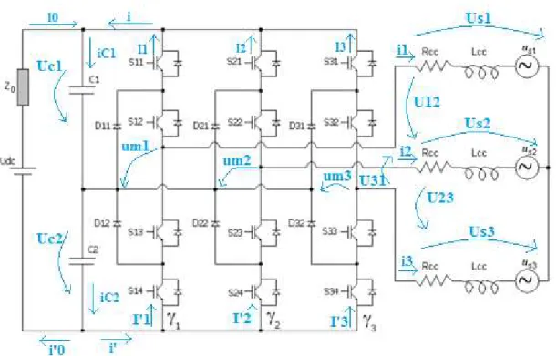
The three-level NPC comprises two capacitors connected in series on the continuous side with three arms. Each arm, represented in figure 3.2, consists of four switches and two diodes connecting to each neutral point. Each switch comprises a power semiconductor with an antiparallel diode in order to guarantee the bidirectional current [21],[24].

Figure 3.2 – NPC monophasic arm

(39)

3.1.1 Switching variables

Each arm of the inverter is characterized by a variable , which quantifies the state of the respective arm ( ), and the state of each switch is characterized by the control variable .

The control of the output voltages or currents of each arm is performed by switching the switches . Each switch has associated two possible states, open ( = 0) or closed ( = 1), being the maximum number of combinations of .

The switches (S11, S14), (S21, S24), (S31, S34) are operating as main switches for PWM, and (S12, S13,), (S22, S23) and (S32, S33) are auxiliary switches to clamp the output terminal potentials to the neutral point potential, together with (D11 – D32).

In three-level inverter, the mid-point of the DC bus provides the third level in the output waveform with the conduction of neutral point diodes.

During these periods, current is drawn from the neutral point. If this point is not connected directly to the supply neutral, then the current is drawn through DC link capacitors, causing one capacitor to charge whilst the other to discharge. Under normal operation, the mean current drawn from the neutral point potential remains constant.

However, during transient operation or if there is any imbalance in the output switching pattern a non-zero mean current will be drawn from the mid-point, resulting in variation of the neutral point voltage.

In fact there are many situations that are not desirable or possible because they violate the topological constraints of circuits theory (short circuit voltage sources, current sources open), thus there are only three combinations between the switches of each arm that allows the three possible voltage levels between the arm of the inverter and neutral point (table 3.1). We obtain this way, distinct states that allow the control of three-phase converter.

Table 3.3 – Available combinations for each arm

1 1 1 0 0

0 0 1 1 0 0

-1 0 0 1 1

Due to topological constraints on the operation of the converter, the switches of each arm must be controlled in a complementary way according to the following relationships:

{

(3.1)

(40)

According to the constraints given by (3.1), representing up to a three-level system the relationship between the state of the command switches ( ) and the value of the variable that characterizes the state of each arm of the three-phase multilevel inverter ( ).

{

Open

(3.2)

Figure 3.3 – 3L-NPC conduction path

(41)

Table 3.2 – Switching commutations

State Voltage

Level

Positive Phase Current

+ _/2 x x

0 0 x x

- - /2 x x

Negative Phase Current

+ _- _/2 x x

0 0 x x

- /2 x x

Switching losses are originated by the commutation processes between the different switch states.

For a positive phase current, the commutation from "+" towards "- (+ → 0 → –) is named “forced commutation”. The contrary natural commutation (–→ 0 → +) realizes a positive output power gradient. They are initiated by an active turn-on transient.

For the following discussion of commutations, a positive phase current is assumed. Only turn-on and turn-off losses of active switches and recovery losses of diodes are considered. For a positive phase current, the commutation (+ → 0) is initiated by the turn-off of and the current is forced from to . After a dead time (to ensure that has completely turned off),

is turned on. The switches and stay on and off respectively.

Table 3.3 – Switch commutations during transitions

State

Positive Phase Current

+↔0 x x

0↔- x x

Negative Phase Current

+↔0 x x

0↔- x x

Only two switches and diodes are involved in this commutation: and

. Essential turn-off

losses occur in . Though the switch is turned on, it does not experience losses since it does not take over any current after the commutation.

(42)

The situation for this pair of commutations is visualized in figure 3.4, where the current path of the switching active device is marked bold and the current path of the switching passive device is marked with a dashed line.

Four devices are involved in the commutation (0 → –). It is started by the active turn-off of the switch , forcing the current from its path through and to

and . has already

been in the on state before; is turned on after a dead time. faces turn-off losses.

Figure 3.4 – 3L-NPC switching transitions

Although the diode in series with is turned off too, it does not experience notable recovery losses since it does not take over voltage after the commutation. Again, for the reverse commutation (–→ 0), all switching transitions take place in the reverse order. is turned off, and is turned on after a dead time. After triggering , the phase current commutates from

and back to and . Both diodes in series and are turned off, but only

(43)

Table 3.4 – Switching transitions losses Switching transition Turn-on losses Turn-off losses Recovery losses

Positive phase current

+↔0 - -

0↔+ -

0↔- - -

-↔0 -

Negative phase current

+↔0 -

0↔+ - -

0↔- -

-↔0 - -

The distribution of the switching losses is summarized in Table 3.3. It is important to note that all commutations in the NPC VSC can be explained by the basic commutation cell, comprising one active switch and one diode.

3.1.2 Voltage and current equations of the converter

By analyzing the circuit of Figure 3.1, we get the following relationships for the AC voltage and currents and of the arm k as a function of the switching variable .

{

(3.3)

{

(3.4)

{

(3.5)

Given the relationships (3.3), (3.4) and (3.5) we obtain the following voltage and current and equations of the converter as function of .

(44)

(

)

(3.7)

(

)

(3.8)

Where:

{

₍

₎

(

)

{

}

{

} (3.9)

3.1.3 Dynamic equations of the converter

By applying the Kirchhoff’s law to the converter of figure 3.1, one obtains the following equations for the currents in the capacitors C1 and C2:

{

∑

(3.9)

Given (3.7) and (3.8) the system of equations (3.10) can be written as a function of switching variables:

{

(3.10)

Considering that,

{

(3.11)

Then the equations (3.11) can be written in function of the voltage on the capacitors:

{

(45)

The system can be written as:

[

] [

]

(3.13)

Where the current is given by:

_(3.14)

represents the internal impedance of the DC voltage source .

The voltages between the arms of the converter (Uij) relate to the simple voltages (Usk) and the voltages between each arm and the neutral point (Umk) by the following equations:

{

(3.15)

Solving the system of equations as a function of the simple voltages (Usk) so as to eliminate the voltages between the arms of the converter (uij), we obtain the following system of equations:

{

(

)

(

)

(

)

(3.16)

By replacing (3.6) in (3.16) we obtain the system (3.17) which relates the voltages applied on the alternating side with the voltages of the capacitors.

{

[(

) (

) ]

[(

) (

) ]

[(

) (

) ]

(46)

The system of equations (3.17) can be represented by matrix system (3.18):

[

]

(3.18)

Where the matrix Ξ is given by:

[

]

[

]

(3.19)

3.1.4 Space vectors

To determine the set of space vectors of the three-level NPC, consider the ideal situation in which the capacitors C1 and C2 of the multilevel converter can be viewed as two voltage sources of equal value:

(3.20)

In this situation, the voltage at the neutral point between the capacitors C1 and C2 is Udc / 2 and neglecting the variation of the voltage on the capacitors, it is found that the relation between the voltages between each arm and the neutral point (Umk) is given by:

(3.21)

The relation (3.21) shows that each arm of the converter can provide between its output and neutral point converter one of three possible voltage values: Udc/2, 0 and -Udc/2. By replacing the equation (3.21) in (3.16) gives the following relationship between the line voltages, measured between two arms of the converter, and the control variables of each arm:

{

(

)

(

)

(

)

(

)

(3.22)

(47)

Table 3.5 – Output voltage levels

Table 3.5 shows that the line voltages between two arms of the converter, can take over five voltage levels, according to the state of each command variable.

Substituting equation (3.21) in the system (3.17), one obtains the relation between the simple voltages (Usk) and the control variables of each arm of the converter:

{

(

)

(

)

(

)

(3.23)

The system (3.22) can also be represented as matrix (3.23).

[

]

[

]

[

]

_(3.23)

By applying the Concordia transformation matrix to the system (3.23) one obtains the vector of output voltages in the α, β components as function of the control variables of each arm in the inverter:

[

] √

[

√ √

] [

]

(3.24)

-1 -1 0 -1 0

-1 1

0 -1

0 0 0

0 1

1 -1

1 0

(48)

The system (3.23) allows to obtain the 3 ^ 3 = 27 distinct states that enable the control of the converter. For each combination of control variables of the arms of the converter, corresponds to a certain vector and consequently the application of a voltage to the converter output.

In table 3.6 are represented twenty-seven vectors provided by the converter three-level NPC in accordance with the state of the arms of the converter, represented by the variable .

It is based on the suitable choice of the value of the control variables that performs control of the quantities desired by applying the proper voltage level. In the control process it is necessary to ensure that the voltage level on the arms of the converter does not transit from one level to the other without passing through intermediate levels, ensuring that the terminals of each switch is not a potential difference applied over a step level voltage.

Table 3.6 – Switching states

Switching State

Voltage

Vector

S1 -1-1-1 V0 ⁄ ⁄ ⁄ 0 0 0

S2 000 V0 0 0 0 0 0 0

S3 111 V0 ⁄ ⁄ ⁄ 0 0 0

S4 0-1-1 V1 0 ⁄ ⁄ ⁄ 0 ⁄ S5 00-1 V2 0 0 ⁄ 0 ⁄ ⁄ S6 -10-1 V3 ⁄ 0 ⁄ ⁄ ⁄ 0 S7 -100 V4 ⁄ 0 0 ⁄ 0 ⁄ S8 -1-10 V5 ⁄ ⁄ 0 0 ⁄ ⁄ S9 0-10 V6 0 ⁄ 0 ⁄ ⁄ 0

S10 100 V1 ⁄ 0 0 ⁄ 0 ⁄

(49)

3.2 Power Semiconductors

System performance highly depends on the semiconductors incorporated. This directly affects efficiency, heat transfer, system voltage and finally cost. It is desirable to use Insulated Gate Bipolar Transistors (IGBT) which is emerging in high power medium voltage applications. The specific cost increases with rated blocking voltage. Moreover, low voltage switches need more current carrying capability, what requires more silicon, to reach the same switching power as high voltage switches. Therefore it can be concluded that a single high voltage chip is more expensive than a low voltage one. Another major indication in chip technology is the specific switching losses.

When using low voltage IGBTs to have less switching losses and lower cost, this will also imply increased conduction losses and increased mechanical and thermal stress on bus bars, cables and protection equipment (circuit breakers etc.). Hence follows that a trade-off needs to be figured out.

3.2.1 Power loss comparison

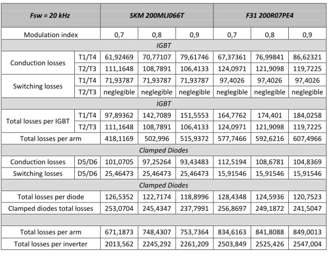
In general, power losses of any power electronic equipment comprise of power losses of all components contained in the equipment. In electrical components the power losses caused in the resistances of these components, so power losses, by nature, means heating of the component. Such an undesirable in the most of applications heating limits the load capabilities and affects either efficiency of the inverter or efficiency of the whole system. In addition, if the temperature of any component of the system exceed a certain acceptable limit due to untransfered heat or overload of the component, it could be finally damaged, which in its turn might cause the failure of the whole system.

For comparison of power losses in a three-level inverter it is enough to compare the maximum power losses. In efficiency point of view, the power losses are averaged over the whole period of the output voltage. The losses are calculated assuming sinusoidal PWM is used.

Most of the power loss occurs in the switches, but there is also some power loss in the DC-link capacitor. The total power loss is:

(3.25) where is the conduction loss of one phase, is the switching loss of one phase, and

is the power loss in the DC-link capacitor.

The evolution of temperature in IGBT modules is a direct consequence of the total losses and imposes the maximum power that can be delivered by power devices or the maximum switching frequency. The following hypotheses were considered to calculate the total losses1 in power devices:

 the load current is sinusoidal;

 the current and voltage ripples are neglected;  the dead times of IGBT modules are neglected.

Manuel Maria Brás Pereira Mascarenhas