A modelling study of the hydrographic structure of the Ross Sea

(1)

OSD

9, 3431–3449, 2012

Ross Sea hydrographic

structure

M. Tonelli et al.

Title Page

Abstract Introduction

Conclusions References

Tables Figures

◭ ◮

Back Close

Full Screen / Esc

Printer-friendly Version Interactive Discussion

Discussion

P

a

per

|

Dis

cussion

P

a

per

|

Discussion

P

a

per

|

Discussio

n

P

a

per

|

Ocean Sci. Discuss., 9, 3431–3449, 2012 www.ocean-sci-discuss.net/9/3431/2012/ doi:10.5194/osd-9-3431-2012

Ocean Science Discussions

This discussion paper is/has been under review for the journal Ocean Science (OS). Please refer to the corresponding final paper in OS if available.

A modelling study of the hydrographic

structure of the Ross Sea

M. Tonelli1, I. Wainer1, and E. Curchitser2

1

Oceanographic Institute, University of Sao Paulo, Praca do Oceanografico, 191, Sao Paulo, SP 05508-120, Brazil

2

Institute of Marine and Coastal Science, Rutgers University, 71 Dudley Rd., New Brunswick, NJ 08901, USA

Received: 15 October 2012 – Accepted: 19 October 2012 – Published: 6 November 2012

Correspondence to: M. Tonelli (mtonelli@usp.br)

(2)

OSD

9, 3431–3449, 2012

structure

M. Tonelli et al.

Title Page

Tables Figures

◭ ◮

Back Close

Full Screen / Esc

Discussion

P

a

per

|

Dis

cussion

P

a

per

|

Discussion

P

a

per

|

Discussio

n

P

a

per

|

Abstract

Dense water formation around Antarctica is recognized as one of the most important processes to climate modulation, since that is where the linkage between the upper and lower limbs of Global Thermohaline Circulation takes place. Assessing whether these processes may be affected by rapid climate changes and all the related feedbacks

5

may be crucial to fully understand the ocean heat transport and to provide future pro-jections. Applying the Coordinated Ocean-Ice Reference (CORE) normal year forcing we have run a 100-yr simulation using Regional Ocean Model System (ROMS) with explicit sea-ice/ice-shelf thermodynamics. The normal year consists of single annual cycle of all the data that are representative of climatological conditions over decades

10

and can be applied repeatedly for as many years of model integration as necessary. The experiment employed a circumpolar variable resolution (1/2◦ _{to 1/24}◦_{) grid}

reach-ing less than 5 km over the inner continental shelf. With Optimum Parameter Analysis (OMP) the main Ross Sea (RS) water masses are identified: Antarctic surface water (AASW), circumpolar deep water (CDW), shelf water (SW) and ice shelf water (ISW).

15

Current configuration allows very realistic representation, where results compare ex-tremely well to the observations.

1 Introduction

The ocean plays a significant role in modulating the global climate transporting heat from lower latitudes to polar regions through Global Thermohaline Circulation (THC;

20

a.k.a. Conveyor Belt), which consist of an upper warm limb and cold deep one (Rintoul, 1991). The linkage of these two branches occurs at specific places around the polar regions, where the warmer limb releases heat to the atmosphere causing the surface water to lose buoyancy and to become denser. This is enhanced by the brine rejection due to sea-ice formation, resulting in cold water sinking and leading to the formation of

25

(3)

OSD

9, 3431–3449, 2012

structure

M. Tonelli et al.

Title Page

Tables Figures

◭ ◮

Back Close

Full Screen / Esc

Discussion

P

a

per

|

Dis

cussion

P

a

per

|

Discussion

P

a

per

|

Discussio

n

P

a

per

|

The Southern Ocean (SO) appears as a key region driving that system, since unique exchange processes and water transformation over the Antarctic continental shelf are responsible for the formation of the Antarctic Bottom Water (AABW); one of the main components of the THC’s lower limb (Orsi et al., 2001, 2002). The main sources of deep waters in the SO are the Weddell Sea (WS) and the Ross Sea (RS), and the

5

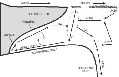
latter one is the formation site of two main AABW components: the high salinity shelf water (HSSW) and the ice shelf water (ISW; Jacobs, 2004; Bergamasco et al., 2004). HSSW production results from the extensive brine rejection in the RS polynya, while ISW is formed under the Ross Sea Ice Shelf (RIS) by means of basal melting. They interact under the RIS to become the densest water masses in the SO and flow towards

10

the the continental shelf break to interact with the Circumpolar Deep Water (CDW), branched offfrom the Antarctic Circumpolar Current (ACC) into the cyclonic Ross Gyre (RG), producing the AABW (Jacobs, 2004; Assmann et al., 2003; Bergamasco et al., 2004). A representative scheme of the circulation under the RIS is shown on Fig. 1, as described by Smethie et al. (2005).

15

1.1 Ross Sea

Facing the Pacific sector of the SO, the RS is approximately centered at 180◦_{W with}

a conic shaped area covering about 5×105 km2between Cape Adare to Cape Colbeck.

Although the average depth is 500 m, there are depressions that reach 1200 m and be-have as dense waters reservoirs, since the shelf break represents the 700 m isobath

20

(Budillon et al., 2003). The ACC follows the continental slope carrying the CDW from east to west and acts as the northern oceanographic boundary of the RS, as the CDW, after being captured by the RG, will be the only heat source to shelf waters strongly in-fluencing the thermohaline circulation of this basin (Budillon and Spezie, 2000; Budillon et al., 2003).

25

(4)

OSD

9, 3431–3449, 2012

structure

M. Tonelli et al.

Title Page

Tables Figures

◭ ◮

Back Close

Full Screen / Esc

Discussion

P

a

per

|

Dis

cussion

P

a

per

|

Discussion

P

a

per

|

Discussio

n

P

a

per

|

the water column salinity and to form the HSSW (Bromwich and Kurtz, 1984; Kurtz and Bromwich, 1985; Jacobs, 2004; Budillon and Spezie, 2000; Bergamasco et al., 2004). The HSSW occupies the lowest layers flowing beneath the RIS to reach the basal ice and mix producing ISW. The newly formed ISW along with the HSSW that did not flow under the RIS will then flow northward to mix with the CDW at the shelf break

produc-5

ing deep and bottom waters (Jacobs et al., 1970; Gordon and Tchernia, 1972; Budillon et al., 1999; Bergamasco et al., 2002a). These processes make HSSW and ISW the most important shelf waters of the RS involved in the formation of the AABW and the deep ocean ventilation.

The low salinity shelf water (LSSW) appears at intermediate depths in the Central

10

Eastern Ross Sea and is believed to result from the interaction between the Antarctic surface water (AASW) and subsurface waters (Jacobs, 2004; Assmann et al., 2003; Bergamasco et al., 2004; Muench et al., 2009). At surface layers, AASW is highly influenced by atmospheric oscillations and sea ice (Jacobs, 2004).

Thus the RS presents a complex, very regional hydrographic structure that is yet

cru-15

cial for the large scale density-driven circulation. Modelling the RS and its deep water mass is a challenge and necessary taste in order to understand the role of southern oceans on climate change.

2 Model description

For this investigation we have used the Regional Ocean Model System (ROMS); a

free-20

surface, terrain-following, hydrostatic primitive equations ocean model (Song and Haid-vogel, 1994). All 2-D and 3-D equations are time-discretized using a third-order accu-rate predictor (Leap-Frog) and corrector (Adams–Molton) time-stepping algorithm. In the horizontal, the primitive equations are evaluated using boundary-fitted, orthogonal curvilinear coordinates on a staggered Arakawa-C grid. In the vertical, the primitive

25

(5)

OSD

9, 3431–3449, 2012

structure

M. Tonelli et al.

Title Page

Tables Figures

◭ ◮

Back Close

Full Screen / Esc

Discussion

P

a

per

|

Dis

cussion

P

a

per

|

Discussion

P

a

per

|

Discussio

n

P

a

per

|

coordinates (Song and Haidvogel, 1994). More detailed descriptions may be found in Budgell (2005) and Wilkin and Hedstrom (1998).

2.1 Experiment setup

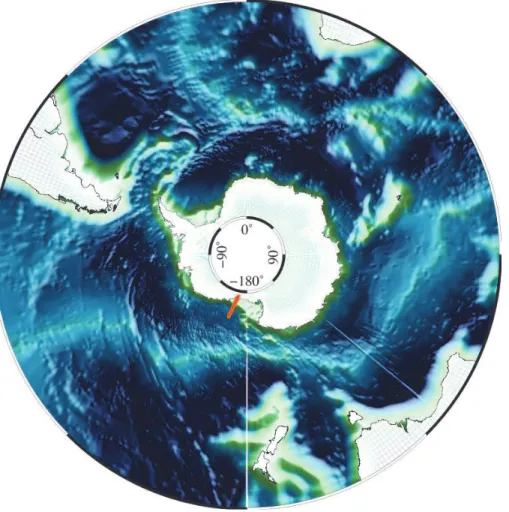
The simulation domain consists of a periodic circumpolar grid between 85.5◦_{S and}

30◦_{S with variable horizontal resolution, reaching less than 5 km over the continental} 5

shelf (Fig. 2). It has a 1/2◦ _{zonal resolution and a varying meridional resolution which}

gradually increases from 1/2◦_{at lower latitudes to 1/24}◦_{at the southernmost boundary,}

resulting in 722×309 grid cells. There are 40 terrain-following vertical levels with higher

resolution near surface and bottom.

For the 3-D momentum advection a 4th order centered scheme is applied in the

10

horizontal and in the vertical. For tracers, a 3rd order upstream horizontal and 4th order centered vertical advection schemes are applied. Biharmonic horizontal mixing of momentum and tracers is used in which the viscosity and diffusivity depend on the grid spacing. Quadratic bottom stress, with a coefficient of 3.0×10−3was applied as a body

force over the bottom layer. The vertical momentum and tracer mixing were handled

15

using the KPP mixing scheme. For computational efficiency, ROMS uses a split-explicit time-stepping scheme in which external (barotropic) and internal (baroclinic) modes are computed separately. The external and internal time step were set to 0.75 and 30 min, respectively in compliance with the Courant, Friedrichs and Lewy (CFL) criterion.

A dynamic-thermodynamic sea-ice module is coupled to the ocean model, having

20

both of them the same grid (Arakawa-C) and time step and sharing the same parallel coding structure (Budgell, 2005). The sea-ice dynamics is based on elastic-viscous-plastic (EVP) rheology (Hunke and Dukowicz, 2002). The sea-ice thermodynamics follows Mellor and Kantha (1989). Two ice layers and a single snow layer is used in the sea-ice module to solve the heat conduction equation. The salt flux underneath the

25

(6)

OSD

9, 3431–3449, 2012

structure

M. Tonelli et al.

Title Page

Tables Figures

◭ ◮

Back Close

Full Screen / Esc

Discussion

P

a

per

|

Dis

cussion

P

a

per

|

Discussion

P

a

per

|

Discussio

n

P

a

per

|

to consider the ice shelves effects on ocean circulation and water mass formation. The ice shelf has a static morphology where thickness and extent do not change. Under the ice shelves, the upper boundary conforms to the ice shelf base and the atmospheric contributions to the momentum and buoyancy fluxes are set to zero. The heat and salt fluxes are calculated as described in Dinniman et al. (2007) with the modification that

5

the heat and salt transfer coefficients are functions of the friction velocity (Holland and Jenkins, 1999).

Two topographic surfaces must be defined for this model configuration: the bottom of the water column and, where necessary, the depth below mean sea level of the ice shelf thickness. Bottom topography was constructed combining ETOPO5 (National

10

Geophysical Data Center – NGDC 1988) and BEDMAP in which sea floor topography is derived from the Smith and Sandwell (1997), ETOPO2 and ETOPO5 (NGDC, 1988). Ice shelf thickness was obtained from the BEDMAP gridded digital model of ice thick-ness (Lythe et al., 2001). Both surfaces were smoothed with a modified Shapiro filter which was designed to selectively smooth areas where the changes in the ice thickness

15

or bottom bathymetry are large with respect to the total depth (Wilkin and Hedstrom, 1998).

The model was initialized with temperature and salinity fields from the January Levi-tus Word Ocean Data 1998 climatology. Under the ice shelf, stable theoretical vertical profiles of temperature and salinity were prescribed as initial conditions to avoid

in-20

stabilities derived from excessive gravity waves at the beginning of the simulation. At the open northern boundary, the model uses the free-surface Chapman condition, the 2-D momentum Flather condition and the 3-D momentum and tracer radiation condi-tion. Temperature and salinity from Levitus 1998 climatology are prescribed as lateral boundary conditions at the open northern boundary.

25

(7)

OSD

9, 3431–3449, 2012

structure

M. Tonelli et al.

Title Page

Tables Figures

◭ ◮

Back Close

Full Screen / Esc

Discussion

P

a

per

|

Dis

cussion

P

a

per

|

Discussion

P

a

per

|

Discussio

n

P

a

per

|

for as many years of model integration as necessary (Large and Yeager, 2004). It in-cludes a 6 hourly 10 m winds, sea level pressure, 10 m specific humidity and 10 m air temperature; the daily solar shortwave radiation flux and downwelling longwave radia-tion flux and the monthly precipitaradia-tion. The air-sea interacradia-tion boundary layer is based on the bulk parameterization of Fairall et al. (1996). It was adapted from the Coupled

5

Ocean-Atmosphere Response Experiment (COARE) algorithm for the computation of surface fluxes of momentum, sensible heat, and latent heat. Surface salinity is relaxed to Levitus climatology with a time scale of 180 days.

2.2 Water masses investigation

To assess water masses representation we have used the Optimum Multiparameter

10

(OMP) analysis, introduced by Tomczak et al. (1981) as an extension ofT S diagram techniques. From a broad perspective, OMP uses Sea Water Types – SWT to solve a linear system of mixture equations and determine the contribution of each water mass encountered at an oceanographic station. OMP assumes a linear mixture model with identical exchange coefficients for all properties (Eq. 1, Tomczak and Large, 1989;

15

Tomczak, 1999; Leffanue and Tomczak, 2004).

    

   

x1θ1+x2θ2+x3θ3+0 =θObs+Rθ x1S1+x2S2+x3S3+0 =SObs+RS x1O1+x2O2+x3O3−∆P V =P VObs+RO x1+x2+x3+0 =1+Rmass

(1)

Scattered T S diagrams created with the 100-yr simulation results were compared against Ross Sea observed data from Orsi and Wiederwohl (2009). This allowed us to determine how ROMS was representing RS water masses and the numerical inherent

20

(8)

OSD

9, 3431–3449, 2012

structure

M. Tonelli et al.

Title Page

Tables Figures

◭ ◮

Back Close

Full Screen / Esc

Discussion

P

a

per

|

Dis

cussion

P

a

per

|

Discussion

P

a

per

|

Discussio

n

P

a

per

|

3 Results

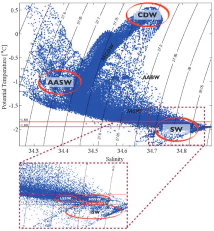
Temperature and salinity data analyzed here refer to the last year of the 100-yr repeat annual cycle run and were were extracted from the cross section along the 165◦_W

longitude (Fig. 2). First step was to build the scatteredθ–S diagram (Fig. 3) in order to validate against observed data of Orsi and Wiederwohl (2009) and to check the water

5

column structure represented by the model. First to be noticed was the overall structure quite similar to Orsi and Wiederwohl (2009), where the warm CDW, fresh AASW and the cold and salty SW can be fairly easy identified. As for most of numerical models, some biases are expected, no matter how good the simulation may be. In that sense, we must point that although the scattered θ–S presents the same triangular-shaped

10

distribution as for Orsi and Wiederwohl (2009), the density field structure appears to be slightly less dense. Orsi and Wiederwohl (2009) suggest the CDW to be between 28.00 and 28.27 kg m−3_{neutral density surfaces, while our results show CDW between}

27.80 and 27.90 kg m−3 _{in agreement with Bergamasco et al. (2002b). Nevertheless,}

these results are consistent with Assmann et al. (2003) numerical experiments where

15

MCDW is centered at the 27.80 kg m−3 _{density layer, while our results show MCDW}

between the 27.75 and 27.80 kg m−3_{density layers.} 3.1 OMP analysis

The scatteredθ–S diagram created with the simulation results was used to obtain the SWTs for the OMP analysis (Table 1). Four water masses properties values were

cho-20

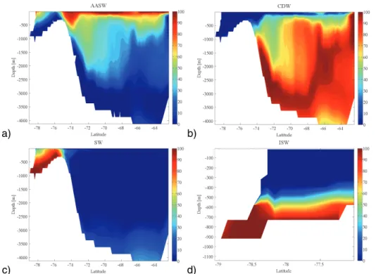
sen considering both the observed data values and the intrinsic model bias in order to assess whether this numerical simulation was able to fully represent the water column structure for this sector of the Ross Sea. The OMP analysis results show water masses contribution maps (%) for AASW, CDW, SW and ISW (Fig. 4).

The AASW (Fig. 4a) occupies the surface layers along almost the whole cross

25

(9)

OSD

9, 3431–3449, 2012

structure

M. Tonelli et al.

Title Page

Tables Figures

◭ ◮

Back Close

Full Screen / Esc

Discussion

P

a

per

|

Dis

cussion

P

a

per

|

Discussion

P

a

per

|

Discussio

n

P

a

per

|

(>90 %) will not show deeper than 200 m, except for the region near the shelf break where AASW reaches 500 m. Some AASW contribution is found in the upper layers over the continental shelf and close to the ice shelf, where sea ice formation will im-pact to transform it into SW to be the densest water mass around Antarctica (Orsi and Wiederwohl, 2009). The saltier MCDW originated by the CDW that eventually makes

5

its way into the continental shelf is also part of this process. MCDW was not individually assessed in this work due to OMP numerical constraints, but an important interaction between AASW and CDW close to the shelf break may also be seen on OMP results (Fig. 4a, b).

As described by Worthington (1981) the CDW (Fig. 4b) appears as the most

volu-10

minous water mass, identified as a thick layer between the upper and colder AASW and the saltier AABW. As CDW is branched from ACC and carried southward by the Antarctic Coastal Current between 160◦_{W and 165}◦_{W (Orsi and Wiederwohl, 2009),}

it is found at intermediate layers from northern limit of the cross sections 65◦_{S to the}

continental slope at 75◦_{S where it is incursion seems to be blocked by AASW near the} 15

shelf break. 34.68 salinity values are consistent with observational data, even though the model has represented CDW half degree colder (0.5◦_{C) than Orsi and Wiederwohl}

(2009) results around 1.0◦_{C. Small CDW contribution values at the bottom layers is}

probably related to the presence of AABW, although this water mass was not sepa-rated in this investigation.

20

Following Orsi and Wiederwohl (2009), we have established the upper limit of the SW (Fig. 4c) as the sudden scatter reduction at−1.85◦C, here centered at the 28.00 kg m−3

density layer a bit less dense than the 28.27 kg m−3_{found by them. Here the SW seems}

to be more restrained to the salinity range of 34.65–34.90 compared to theS >34.50 suggested by Orsi and Wiederwohl (2009), what makes these pretty consistent results.

25

(10)

OSD

9, 3431–3449, 2012

structure

M. Tonelli et al.

Title Page

Tables Figures

◭ ◮

Back Close

Full Screen / Esc

Discussion

P

a

per

|

Dis

cussion

P

a

per

|

Discussion

P

a

per

|

Discussio

n

P

a

per

|

2009; Orsi and Wiederwohl, 2009), the formation and export of the SW and its compo-nents occurs in pulses related to the polynyas recurrence. Another feature to be noticed is the very light contribution of the SW on the oceanic basin 4000 m, where the AABW takes place. Since the AABW results from the interaction of the SW and the CDW near the shelf break, these results suggest that the model may be reproducing important

5

processes such as the AABW formation.

The ISW (Fig. 4d) occupies the bottom layers over the continental shelf and deepens towards the base of the ice shelf. Observational studies such as Budillon et al. (2003) point that the ISW spreads along the deep layers of the shelf, but over a thin layer of HSSW, which agrees with the believed formation process describe in Fig. 1 for the

10

ISW. They discuss that from the 400 m depth to the bottom of the continental shelf there is essentially a mixture of HSSW and ISW that reach to shelf break to take part in the formation of the AABW. As suggested by Jacobs (2004) the ISW is defined as being colder than the sea water freezing point (at surface) with its formation occurring by means of melting at the RIS base. Although the ice shelf used in this simulation is

15

static in time, its thermodynamic is enough to reproduce such melting processes. Here, as for Holland et al. (2003) numerical experiment, ISW definition includes all seawater colder than−1.95◦C (they used−1.90◦C) which may have lead ISW to be represented

at both deep and bottom layers on the continental shelf.

4 Conclusions 20

The aim of this work was to assess the representation of the RS water masses with a regional ocean model with an active sea ice/ice shelf thermodynamic parametriza-tion. Results suggest that the numerical investigations of such an isolated environment as the cavity beneath the RIS is not only feasible but much useful to understand the oceanographic processes related to water transformation under the ice shelves.

Us-25

(11)

OSD

9, 3431–3449, 2012

structure

M. Tonelli et al.

Title Page

Tables Figures

◭ ◮

Back Close

Full Screen / Esc

Discussion

P

a

per

|

Dis

cussion

P

a

per

|

Discussion

P

a

per

|

Discussio

n

P

a

per

|

and ISW. These results are consistent with observations (Bergamasco et al., 2002a; Budillon et al., 2003; Orsi and Wiederwohl, 2009).

AASW was represented at the surface layers with salinity ranging from 34.30 to 34.45 and temperature centered at −1.0◦C. The warmer (0.5◦C) and saltier (34.68)

CDW was represented as the most voluminous water mass spreading along

interme-5

diate layers, following the slope and reaching the outer portion of the shelf break. The SW appeared ate the bottom layers of the continental shelf, trapped by topography but still able to reach the shelf break with its characteristic low temperature (−1.85◦C) and

high salinity (34.65–34.90). Finally the model was also able to represent the super-cooled ISW with temperatures below −1.95◦C. These are remarkable results, since

10

SW and its components are the most important water masses in the RS involved in the deep world ocean ventilation as they will interact with CDW to form the AABW. OMP analysis has provided a good spacial description of the RS water masses and works as an objective method for characterizing polar oceans. Since we have used only salin-ity and temperature as input for OMP only three water masses could be separated.

15

We are currently using potential vorticity as an additional input to the OMP method which results in the identification of 4 water masses. Moreover, this investigation con-stitutes a starting point to further experimentations: first applying an interannual forcing to investigate the temporal evolution of water masses; secondly improving the ice shelf physics in the code.

20

Acknowledgements. To Virna Meccia for providing great help setting this experiment up and running, CNPq, FAPESP, CAPES and INCT-Criosfera.

References

Assmann, K., Hellmer, H., and Beckmann, A.: Seasonal variation in circulation and water mass distribution on the Ross Sea continental shelf, Antarct. Sci., 15, 3–11, 2003. 3433, 3434,

25

(12)

OSD

9, 3431–3449, 2012

structure

M. Tonelli et al.

Title Page

Tables Figures

◭ ◮

Back Close

Full Screen / Esc

Discussion

P

a

per

|

Dis

cussion

P

a

per

|

Discussion

P

a

per

|

Discussio

n

P

a

per

|

Bergamasco, A., Defendi, V., and Meloni, R.: Some dynamics of water outflow from beneath the Ross Ice Shelf during 1995 and 1996, Antarct. Sci., 14, 74–82, 2002a. 3434, 3441 Bergamasco, A., Defendi, V., Zambianchi, E., and Spezie, G.: Evidence of dense water overflow

on the Ross Sea shelf-break, Antarct. Sci., 14, 271–277, 2002b. 3438

Bergamasco, A., Defendi, V., Budillon, G., and Spezie, G.: Downslope flow observations near Cape Adare shelf-break, Antarct. Sci., 16, 199–204, 2004. 3433, 3434

5

Bromwich, D. and Kurtz, D.: Katabatic wind forcing of the Terra Nova Bay polynya, J. Geophys. Res., 89, 3561–3572, 1984. 3434

Budgell, W.: Numerical simulation of ice–ocean variability in the Barents Sea region, Ocean Dynam., 55, 370–387, 2005. 3435

Budillon, G. and Spezie, G.: Thermohaline structure and variability in the Terra Nova Bay

10

polynya, Ross Sea, Antarct. Sci., 12, 493–508, 2000. 3433, 3434

Budillon, G., Tucci, S., Artegiani, A., and Spezie, G.: Water Masses and Suspended Matter Characteristics of the Western Ross Sea, Ross Sea Ecology, Springer, Berlin, 63–81, 1999. 3434

Budillon, G., Pacciaroni, M., Cozzi, S., Rivaro, P., Catalano, G., Ianni, C., and Cantoni, C.: An

15

optimum multiparameter mixing analysis of the shelf waters in the Ross Sea, Antarct. Sci., 15, 105–118, 2003. 3433, 3439, 3440, 3441

Dinniman, M., Klinck, J., and Smith Jr., W.: Influence of sea ice cover and icebergs on circulation and water mass formation in a numerical circulation model of the Ross Sea, Antarctica, J. Geophys. Res., 112, C11013, doi:10.1029/2006JC004036, 2007. 3436

20

Fairall, C., Bradley, E., Rogers, D., Edson, J., and Youngs, G.: Bulk parameterization of air– sea fluxes for Tropical Ocean-Global Atmosphere Coupled-Ocean Atmosphere Response, J. Geophys. Res., 101, 3747–3764, 1996. 3437

Gordon, A.: Interocean exchange of thermocline water, J. Geophys. Res., 91, 5037–5046, 1986. 3432

25

Gordon, A. and Tchernia, P.: Waters of the continental margin off Adelie Coast, Antarctica, Antarct. Oceanol., 2, 59–69, 1972. 3434

Holland, D. and Jenkins, A.: Modeling thermodynamic ice–ocean interactions at the base of an ice shelf, J. Phys. Oceanogr., 29, 1787–1800, 1999. 3436

Holland, D. and Jenkins, A.: Adaptation of an isopycnic coordinate ocean model for the study

30

(13)

OSD

9, 3431–3449, 2012

structure

M. Tonelli et al.

Title Page

Tables Figures

◭ ◮

Back Close

Full Screen / Esc

Discussion

P

a

per

|

Dis

cussion

P

a

per

|

Discussion

P

a

per

|

Discussio

n

P

a

per

|

Holland, D., Jacobs, S., and Jenkins, A.: Modelling the ocean circulation beneath the Ross Ice Shelf, Antarct. Sci., 15, 13–23, 2003. 3439, 3440

Hunke, E. and Dukowicz, J.: The elastic-viscous-plastic sea ice dynamics model in general orthogonal curvilinear coordinates on a sphere-incorporation of metric terms, Mon. Weather Rev., 130, 1848–1865, 2002. 3435

5

Jacobs, S.: Bottom water production and its links with the thermohaline circulation, Antarct. Sci., 16, 427–437, 2004. 3433, 3434, 3440

Jacobs, S., Amos, A., and Bruchhausen, P.: Ross Sea oceanography and Antarctic bottom water formation, in: Deep Sea Research and Oceanographic Abstracts, Vol. 17, Elsevier, Pergamon Press, UK, 935–962, 1970. 3434

10

Kurtz, D. and Bromwich, D.: A recurring, atmospherically forced polynya in Terra Nova Bay, in: Oceanology of the Antarctic Continental Shelf, edited by: Jacobs, S. S., Antarctic Research Series 43, American Geophysical Union, Washington, DC, 177–201, 1985. 3434

Large, W. and Yeager, S.: Diurnal to decadal global forcing for ocean and sea-ice models: the data sets and flux climatologies, National Center for Atmospheric Research, 2004. 3436,

15

3437

Leffanue, H. and Tomczak, M.: Using OMP analysis to observe temporal variability in water mass distribution, J. Mar. Syst., 48, 3–14, 2004. 3437

Lythe, M. B., Vaughan, D. G., and the BEDMAP Consortium: BEDMAP: a new ice thickness and subglacial topographic model of Antarctica, J. Geophys. Res., 106, 11335–11351, 2001.

20

3436

Mellor, G. and Kantha, L.: An ice–ocean coupled model, J. Geophys. Res., 94, 10937–10954, doi:10.1029/JC094iC08p10937, 1989. 3435

Muench, R., Padman, L., Gordon, A., and Orsi, A.: A dense water outflow from the Ross Sea, Antarctica: mixing and the contribution of tides, J. Mar. Syst., 77, 369–387, 2009. 3434, 3439

25

Orsi, A. and Wiederwohl, C.: A recount of Ross Sea waters, Deep-Sea Res. Pt. II, 56, 778–795, 2009. 3437, 3438, 3439, 3440, 3441

Orsi, A., Jacobs, S., Gordon, A., and Visbeck, M.: Cooling and ventilating the abyssal ocean, Geophys. Res. Lett, 28, 2923–2926, 2001. 3433

Orsi, A., Smethie Jr., W., and Bullister, J.: On the total input of Antarctic waters to the deep

30

ocean: a preliminary estimate from chlorofluorocarbon measurements, J. Geophys. Res, 107, 3122, doi:10.1029/2001JC000976, 2002. 3433

(14)

OSD

9, 3431–3449, 2012

structure

M. Tonelli et al.

Title Page

Tables Figures

◭ ◮

Back Close

Full Screen / Esc

Discussion

P

a

per

|

Dis

cussion

P

a

per

|

Discussion

P

a

per

|

Discussio

n

P

a

per

|

Smethie, W., Jacobs, S. and Jacobs, S: Circulation and melting under the Ross Ice Shelf: estimates from evolving CFC, salinity and temperature fields in the Ross Sea, Deep-Sea Res. Pt. I, 52, 959–978, 2005. 3433

Smith, W. and Sandwell, D.: Global sea floor topography from satellite altimetry and ship depth

5

soundings, Science, 277, 1956–1962, 1997. 3436

Song, Y. and Haidvogel, D.: A semi-implicit ocean circulation model using a generalized topography-following coordinate system, J. Comput. Phys., 115, 228–244, 1994. 3434, 3435 Tomczak, M.: Some historical, theoretical and applied aspects of quantitative water mass

anal-ysis, J. Mar. Res., 57, 275–303, 1999. 3437

10

Tomczak, M. and Large, D.: Optimum multiparameter analysis of mixing in the thermocline of the eastern Indian Ocean, J. Geophys. Res., 94, 16141–16149 doi:10.1029/JC094iC11p16141, 1989. 3437

Tomczak Jr., M.: A multi-parameter extension of temperature/salinity diagram techniques for the analysis of non-isopycnal mixing, Prog. Oceanogr., 10, 147–171, 1981. 3437

15

Wilkin, J. and Hedstrom, K.: User’s manual for an orthogonal curvilinear grid-generation pack-age, Institute of Marine and Coastal Sciences, Rutgers University, available at: http://www. marine.rutgers.edu/po/tools/gridpak/grid manual.ps.gz, last access: 11 August 2004,1998. 3435, 3436

Worthington, L.: The water masses of the world ocean: some results of a fine-scale census, in: Evolution of Physical Oceanography: Scientific Surveys in Honor of Henry Stommel, edited by: Warren, B. A. and Wunsch, C., MIT Press, Cambridge, 6–41, 1981. 3439

(15)

OSD

9, 3431–3449, 2012

structure

M. Tonelli et al.

Title Page

Tables Figures

◭ ◮

Back Close

Full Screen / Esc

Discussion

P

a

per

|

Dis

cussion

P

a

per

|

Discussion

P

a

per

|

Discussio

n

P

a

per

|

Table 1.Sea Water Types derived fromT Sdiagram.

Water Mass Salinity Temperature

AASW 34.37 −1.0

SW 34.78 <−1.85

ISW 34.78 <−1.95

(16)

OSD

9, 3431–3449, 2012

structure

M. Tonelli et al.

Title Page

Tables Figures

◭ ◮

Back Close

Full Screen / Esc

Discussion

P

a

per

|

Dis

cussion

P

a

per

|

Discussion

P

a

per

|

Discussio

n

P

a

per

|

Fig. 1. Schematic representation of the circulation under the Ross Sea Ice Shelf. AASW:

(17)

OSD

9, 3431–3449, 2012

structure

M. Tonelli et al.

Title Page

Tables Figures

◭ ◮

Back Close

Full Screen / Esc

Discussion

P

a

per

|

Dis

cussion

P

a

per

|

Discussion

P

a

per

|

Discussio

n

P

a

per

|

Fig. 2.Simulation domain – variable resolution grid reaching less than 5 km over the continental

(18)

OSD

9, 3431–3449, 2012

structure

M. Tonelli et al.

Title Page

Tables Figures

◭ ◮

Back Close

Full Screen / Esc

Discussion

P

a

per

|

Dis

cussion

P

a

per

|

Discussion

P

a

per

|

Discussio

n

P

a

per

|

Fig. 3.ScatteredT S diagram created with the simulation results showing the main Ross Sea

(19)

OSD

9, 3431–3449, 2012

structure

M. Tonelli et al.

Title Page

Tables Figures

◭ ◮

Back Close

Full Screen / Esc

Discussion

P

a

per

|

Dis

cussion

P

a

per

|

Discussion

P

a

per

|

Discussio

n

P

a

per

|

a) b)

c) d)

Fig. 4. (a)Antarctic surface water (AASW) spacial contribution (%) at the meridional section

along the 165◦_{W Latitude.} _(b)_{Circumpolar deep water (CDW) spacial contribution (%) at the}

meridional section along the 165◦_{W Latitude.}_(c)_{Shelf water (SW) spacial contribution (%) at}

the meridional section along the 165◦_{W Latitude.}_(d)_{Ice shelf water (ISW) spacial contribution}