Ice-shelf forced vibrations modelled with a full 3-D elastic model

(1)

TCD

8, 6059–6078, 2014

Ice-shelf forced vibrations modelled with a full 3-D elastic

model

Y. V. Konovalov

Title Page

Abstract Introduction

Conclusions References

Tables Figures

◭ ◮

Back Close

Full Screen / Esc

Printer-friendly Version Interactive Discussion

Discussion

P

a

per

|

Discussion

P

a

per

|

Discussion

P

a

per

|

Discussion

P

a

per

|

The Cryosphere Discuss., 8, 6059–6078, 2014 www.the-cryosphere-discuss.net/8/6059/2014/ doi:10.5194/tcd-8-6059-2014

This discussion paper is/has been under review for the journal The Cryosphere (TC). Please refer to the corresponding final paper in TC if available.

Ice-shelf forced vibrations modelled with

a full 3-D elastic model

Y. V. Konovalov

Department of Mathematics, National Research Nuclear University “MEPhI”, Kashirskoe shosse 31, 115409 Moscow, Russia

Received: 19 October 2014 – Accepted: 14 November 2014 – Published: 5 December 2014

Correspondence to: Y. V. Konovalov (yu-v-k@yandex.ru)

(2)

TCD

8, 6059–6078, 2014

model

Y. V. Konovalov

Title Page

Tables Figures

◭ ◮

Back Close

Full Screen / Esc

Discussion

P

a

per

|

Discussion

P

a

per

|

Discussion

P

a

per

|

Discussion

P

a

per

|

Abstract

Ice-shelf forced vibrations modelling was performed using a full 3-D finite-difference elastic model, which takes into account sub-ice seawater flow. The sub-ice seawater flow was described by the wave equation, so the ice-shelf flexures result from the hy-drostatic pressure perturbations in sub-ice seawater layer. The numerical experiments

5

were performed for idealized ice-shelf geometry, which was considered in the numerical experiments in Holdsworth and Glynn (1978). The ice-plate vibrations were modelled for harmonic ingoing pressure perturbations and for a wide spectrum of the ocean swell periodicities, ranging from infragravity wave periods down to periods of a few seconds (0.004–0.2 Hz). The spectrums for the vibration amplitudes were obtained in this range

10

and are published in this manuscript. The spectrums contain distinct resonant peaks, which corroborate the ability of resonant-like motion in suitable conditions of the forcing. The impact of local irregularities in the ice-shelf geometry to the amplitude spectrums was investigated for idealized sinusoidal perturbations of the ice surface and the sea bottom. The results of the numerical experiments presented in this manuscript, are

15

approximately in agreement with the results obtained by the thin-plate model in the re-search carried out by Holdsworth and Glynn (1978). In addition, the full model allows to observe 3-D effects, for instance, vertical distribution of the stress components in the plate. In particular, the model reveals the increasing in shear stress, which is neglected in the thin-plate approximation, from the terminus towards the grounding zone with the

20

(3)

TCD

8, 6059–6078, 2014

model

Y. V. Konovalov

Title Page

Tables Figures

◭ ◮

Back Close

Full Screen / Esc

Discussion

P

a

per

|

Discussion

P

a

per

|

Discussion

P

a

per

|

Discussion

P

a

per

|

1 Introduction

Tides and ocean swells produce ice shelf bends and, thus, they can initiate break-up of sea-ice in the marginal zone (Holdsworth and Glynn, 1978; Goodman et al., 1980; Wadhams, 1986; Squire et al., 1995; Meylan et al., 1997; Turcotte and Schubert, 2002) and also they can excite ice-shelf rift propagation. Strong correlations between

5

rift propagation rate and ocean swells impact have not revealed (Bassis et al., 2008), and it is not clear to what degree rift propagation can potentially be triggered by tides and ocean swells. Nevertheless, the impacts of tides and of ocean swells are the parts of the total force (Bassis et al., 2008) that produces sea-ice calving processes in ice shelves (MacAyeal et al., 2006). Thus, the understanding of vibrating processes in

10

ice shelves is important from the point of view of investigations of ice-sheet-ocean interaction and of sea level change due to alterations in the rate of sea-ice calving.

The modelling of ice-shelf bends and of ice-shelf vibrations were developed, e.g. in Holdsworth and Glynn (1978), Goodman et al. (1980), Wadhams (1986), Vaughan (1995), Turcotte and Schubert (2002), using the approximation of a thin plate. These

15

models allow to simulate ice-shelf deflections and to obtain bending stresses emerging due to the vibrating processes, and to assess possible effects of tides and ocean swells impacts on the calving process. Further development of elastic-beam models for de-scription of ice-shelf flexures implies the application of visco-elastic rheological models. In particular, tidal flexures of ice-shelf were obtained using linear visco-elastic Burgers

20

model in Reeh et al. (2003) and using the nonlinear 3-D visco-elastic full Stokes model in Rosier et al. (2014).

Ice-stream response to ocean tides was described by full Stokes 2-D finite-element employing a non-linear visco-elastic Maxwell rheological model by Gudmundsson (2011). This modelling work revealed that tidally induced ice-stream motion is strongly

25

(4)

TCD

8, 6059–6078, 2014

model

Y. V. Konovalov

Title Page

Tables Figures

◭ ◮

Back Close

Full Screen / Esc

Discussion

P

a

per

|

Discussion

P

a

per

|

Discussion

P

a

per

|

Discussion

P

a

per

|

(MSf) through a nonlinear interaction between the main semi-diurnal tidal components (Gudmundsson, 2011).

A 2-D finite-element flow-line model with an elastic rheology was developed by O. V. Sergienko (Bromirski et al., 2010; Sergienko, 2010) and was used to estimate mechan-ical impact of high-frequency tidal action on stress regime of ice shelves. In this model

5

seawater was considered as incompressible, inviscid fluid and was described by the velocity potential.

In this work, the modelling of forced vibrations of a buoyant, uniform, elastic ice-shelf, which floats in shallow water of variable depth, is developed. The simulations of bends of ice-shelf are performed by a full 3-D finite-difference elastic model. The

10

main aim of this work is to derive the eigen-frequencies of the system, which includes the buoyant, elastic ice-shelf and the sea water under the ice-shelf, implying that, in suitable conditions a resonant-like vibration can be induced by the incident ocean wave (Holdsworth and Glynn, 1978; Bromirski et al., 2010). In other words, here we consider the same mechanism for generating the bending stresses at locations along an

ice-15

shelf far from the grounding zone due to vibration of the ice-shelf in a mode higher than the fundamental (nontidal theory for ice-shelf fracture), like was considered in (Holdsworth and Glynn, 1978). Furthermore, the attempt to apply the general elastic theory instead of well-developed thin plate theory is launched here (in 3-D case).

2 Field equations

20

2.1 Basic equations

(5)

TCD

8, 6059–6078, 2014

model

Y. V. Konovalov

Title Page

Tables Figures

◭ ◮

Back Close

Full Screen / Esc

Discussion

P

a

per

|

Discussion

P

a

per

|

Discussion

P

a

per

|

Discussion

P

a

per

|

     

    

∂σxx

∂x +

∂σxy

∂y +

∂σxz

∂z =ρ

∂2U ∂t2;

∂σyx

∂x +

∂σyy

∂y +

∂σyz

∂z =ρ

∂2V ∂t2;

∂σ_zx

∂x +

∂σzy

∂y +

∂σ_zz

∂z =ρ∂

2

W ∂t2 ;

0< x < L;y1(x)< y < y2(x);hb(x,y)< z < hs(x,y)

(1)

where (x,y,z) is a rectangular coordinate system with thexaxis along the central line, and thezaxis pointing vertically upward;U,V andW are two horizontal and vertical ice displacements, respectively;σi j are the stress components; ρis ice density; hb(x,y),

hs(x,y) are ice bed and ice surface elevations, respectively; L is the glacier length 5

along the central line;y1(x),y2(x) are the lateral edges. In a common case of arbitrary

ice-shelf geometry, is supposed that thex axis direction is chosen so that the lateral edges can be approximated by single-value functions (y1(x),y2(x)).

The sub-ice water is considered as an incompressible and nonviscous fluid of uni-form density. Additional assumption is that the water depth changes slowly in horizontal

10

directions. Under these assumptions the sub-ice water flows uniformly in a vertical col-umn, and the manipulation with the continuity equation and the Euler equation yields the wave equation (Holdsworth and Glynn, 1978)

∂2Wb

∂t2 =

1

ρw

∂ ∂x

d0

∂P′ ∂x

+_ρ1

w

∂ ∂y

d0

∂P′ ∂y

; (2)

whereρwis sea water density;d0(x,y) is the depth of the sub-ice water layer;Wb(x,y,t) 15

is the ice-shelf base vertical deflection, andWb(x,y,t)=W(x,y,hb,t);P

′

(x,y,t) is the deviation from the hydrostatic pressure.

For harmonic vibrations the method of separation of variables yields the same equa-tions, in which only the operator _∂t∂22 should be replaced with the−ω

2

, where ωis the frequency of the vibrations, – for thex,y,z dependent values. Likewise, the

deforma-20

(6)

TCD

8, 6059–6078, 2014

model

Y. V. Konovalov

Title Page

Tables Figures

◭ ◮

Back Close

Full Screen / Esc

Discussion

P

a

per

|

Discussion

P

a

per

|

Discussion

P

a

per

|

Discussion

P

a

per

|

as well as the suitable terms in the boundary conditions listed below are absent in the final equations formulated for the vibration problem, for which the method of separation of variables is applied.

2.2 Boundary conditions

The boundary conditions are (i) stress free ice surface, (ii) normal stress exerted by

5

seawater at the ice-shelf free edges and at the ice-shelf base, (iii) rigidly fixed edge at the origin of the ice-shelf (i.e. in the glacier along the grounding line). In detail, well-known form of the boundary conditions, for example, at the ice-shelf base is expressed as

   

  

σ_xz =σ_xx∂hb

∂x +σxy

∂h_b

∂y +P

∂h_b ∂x; σyz=σyx

∂h_b

∂x +σyy

∂h_b

∂y +P

∂h_b ∂y; σ_zz=σ_zx∂hb

∂x +σzy

∂h_b ∂y −P;

(3)

10

whereP is the pressure (P =ρgH+P′,H is ice-shelf thickness).

In the model, developed here, we considered the approach, in which the known boundary conditions (Eq. 3) have been incorporated into the basic Eq. (1). A suitable form of the equations can be written after discretization of the model (Konovalov, 2012) and is shown below.

15

In the ice-shelf forced vibration problem the boundary conditions for the water layer are (i) at the boundaries coincided to the lateral free edges:∂P_∂ ′

n =0, wherenis the unit

horizontal vector normal to the edges; (ii) at the boundary along the grounding line: ∂P′

∂n =0, wheren is the unit horizontal vector normal to the grounding line; and (iii) at

the ice-shelf terminus the pressure perturbations are excited by the periodical impact

20

(7)

TCD

8, 6059–6078, 2014

model

Y. V. Konovalov

Title Page Abstract Introduction Conclusions References Tables Figures ◭ ◮ ◭ ◮ Back Close

Full Screen / Esc

Printer-friendly Version Interactive Discussion Discussion P a per | Discussion P a per | Discussion P a per | Discussion P a per |

2.3 Discretization of the model

The numerical solutions were obtained by a finite-difference method, which based on the coordinate transformationx,y,z→x,η= y−y1

y₂−y₁,ξ=(hs−z)/H(e.g. Hindmarsh and

Hutter, 1988; Blatter, 1995; Hindmarsh and Payne, 1996; Pattyn, 2003). The coordinate transformation transfigures an arbitrary ice domain into the rectangular parallelepiped

5

Π ={0≤x≤L; 0≤η≤1; 0≤ξ≤1}.

The numerical experiments with ice flow models and with elastic models (Konovalov, 2012, 2014) have shown that the method, in which the initial boundary conditions (Eq. 3) being included in the momentum Eq. (1), can be applied in the finite-difference models. In certain cases, the approach additionally provides the numerical stability of

10

the solution. In this work the method has been applied in the developed 3-D elastic model. For instance, after the coordinate transformation, the applicable equations at ice-shelf base can be written as follows

_∂σ xx ∂x Nξ +

η′_x∂σxx ∂η

Nξ

+

ξ′_x∂σxx ∂ξ

Nξ

+ η′_y∂σxy ∂η

!Nξ

+ ξ_y′∂σxy ∂ξ

!Nξ

(4)

− 1

H

1 2∆ξσ

N_ξ−2

xz +

1

H

4 2∆ξσ

N_ξ−1

xz −

1

H

3 2∆ξ

σxx ∂hb

∂x +σxy

∂hb ∂y Nξ 15 − 1 H 3 2∆ξP

′∂hb

∂x ≈

3 2∆ξρg

∂hb

∂x +ρ

∂2U ∂t2

!Nξ

;

∂σ_yx ∂x

!Nξ

+ η′_x∂σyx ∂η

!Nξ

+ ξ_x′∂σyx ∂ξ

!Nξ

+ η′_y∂σyy ∂η

!Nξ

+ ξ′_y∂σyy ∂ξ

!Nξ

− 1

H

1 2∆ξσ

Nξ−2

yz +

1

H

4 2∆ξσ

Nξ−1

yz −

1

H

3 2∆ξ

σ_yx∂hb

∂x +σyy

∂hb

∂y

(8)

TCD

8, 6059–6078, 2014

model

Y. V. Konovalov

Title Page Abstract Introduction Conclusions References Tables Figures ◭ ◮ ◭ ◮ Back Close

Full Screen / Esc

Printer-friendly Version Interactive Discussion Discussion P a per | Discussion P a per | Discussion P a per | Discussion P a per | − 1 H 3 2∆ξP

′∂hb

∂y ≈

3 2∆ξρg

∂hb

∂y +ρ

∂2V ∂t2

!Nξ

; _∂σ zx ∂x Nξ +

η′x ∂σ_zx

∂η

Nξ

+

ξx′ ∂σ_zx

∂ξ

Nξ

+ η′y ∂σzy

∂η

!Nξ

+ ξy′ ∂σzy

∂ξ

!Nξ

−

1

H

1 2∆ξσ

N_ξ−2

zz +

1

H

4 2∆ξσ

N_ξ−1

zz −

1

H

3 2∆ξ

σzx ∂hb

∂x +σzy

∂hb ∂y Nξ + 1 H 3 2∆ξP

′_{≈ −} 3

2∆ξρg+ρg+ρ ∂2W

∂t2 !Nξ

;

where index “Nξ” corresponds to grid layer located at the ice shelf base. Thus, the

5

stress componentsσ_xz,σ_yz,σ_zz at theN_ξ-layer have been replaced in the basic Eq. (1) in agreement with the boundary conditions (Eq. 3). The same manipulations were per-formed with the equations at the free edges and on the free surface.

2.4 Equations for ice-shelf displacements

Constitutive relationships between stress tensor components and displacements

cor-10

respond to Hook’s law (e.g. Landau and Lifshitz, 1986; Lurie, 2005):

σ_{i j}= E

1+ν

u_{i j}+ ν

1−2νul lδi j

, (5)

whereui j are the strain components.

Substitution of these relationships into Eqs. (1) and (4) gives final equations of the model.

(9)

TCD

8, 6059–6078, 2014

model

Y. V. Konovalov

Title Page

Tables Figures

◭ ◮

Back Close

Full Screen / Esc

Discussion

P

a

per

|

Discussion

P

a

per

|

Discussion

P

a

per

|

Discussion

P

a

per

|

3 Results of the numerical experiments

The numerical experiments with ice-shelf forced vibrations were carried out for a phys-ically idealized ice plate with trapezoidal profile (Fig. 1a). The ice plate is 14 km long, 1.5 km wide and ice thickness decreases from 355 to 71 m. This tapering ice plate approximately coincides with the shape of the Erebus Glacier Tongue, which was

con-5

sidered in the free vibration problem in Holdsworth and Glynn (1978). Figure 1b and d shows the “rolled” ice surface and the “bumpy” seabed, respectively. These comple-mentary geometries were considered with intent to investigate the impact of the pertur-bations on the spectrums (on the eigen-frequencies of the system). In the experiment with rolled surface, in fact, the sinusoidally perturbations of the ice-shelf thickness were

10

considered and were expressed as

H=H0+ ∆H0+ ∆Hsin(n2πx/L) , (6)

whereH0is the origin ice-shelf thickness. Thus, the surface elevation in Fig. 1b varies

in agreement with the expressionhs=H

1−_ρρ

w

.

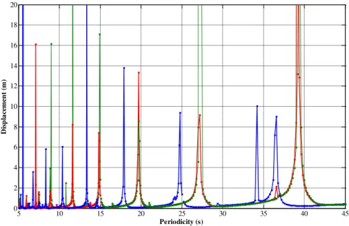
Figure 2 shows the amplitude spectrums (amplitudes of the flexures vs. the

frequen-15

cies of the vibrations). The peaks in Fig. 2 correspond to the eigen-frequencies of the system, which includes ice-shelf and sub-ice water layer. About nine resonant peaks la-belled in Fig. 2, can be distinguished in the part of the spectrum, which corresponds to the ocean swells with periods from 5 to 45 s. For instance, we can select three eigen-frequencies, which are close to those that were selected in Holdsworth and Glynn

20

(1978). They are approximately equal to 0.067, 0.051, 0.037 Hz, respectively. The cor-responding periodicities are equal to 14.9, 19.7, 27.1 s vs. the periodicities of 16.0, 20.2, 24.2 s derived in the thin-plate model in Holdsworth and Glynn (1978), i.e. the relative deviation does not exceed 12 %.

Curves 2 and 3 are the amplitude spectrums, which were obtained for the “rolled” ice

25

(10)

TCD

8, 6059–6078, 2014

model

Y. V. Konovalov

Title Page

Tables Figures

◭ ◮

Back Close

Full Screen / Esc

Discussion

P

a

per

|

Discussion

P

a

per

|

Discussion

P

a

per

|

Discussion

P

a

per

|

which reveals some shifts of the amplitude peaks and/or appearance of complemen-tary peaks in comparison with the basic spectrum. The shifts of peaks are observed in the case of “rolled” surface (curve 1 and curve 2 in Fig. 2). This impact is the result of the change in ice-shelf effective thickness (in the model the change is equal to∆H0 in

Eq. 6). In the case of “bumpy” sea bed the resonant peaks are aligned with the peaks

5

in the basic spectrum (curve 1 and curve 3 in Fig. 2), but the complementary peaks appear in the spectrum.

The flexures of the ice-plate for the three selected modes are shown in Fig. 3, re-spectively.

The number of nodes/antinodes in Fig. 3 inx direction roughly corresponds to the

10

number of the ones, which can be distinguished in the flexures shown in Fig. 2 in Holdsworth and Glynn (1978).

Figure 4 shows the longitudinal stress component σ_xx and the shear stress com-ponentσxz, respectively, along the centerline for the second mode shown in Fig. 3b. Maxima/minima of the longitudinal stress coincide with the antinodes, vice versa,

max-15

ima/minima of the shear stress coincide with the nodes (Fig. 4). The magnitude of the shear stress in the maxima/minima an order less than the magnitude of the longitudinal stress (Fig. 4).

4 Summary

The ice-shelf forced vibrations modelling can be performed by 3-D full elastic model,

20

although the volume of the routine sufficiently increases in comparison with the thin-plate model.

The numerical experiments have shown the impact of ice surface/sea bottom topog-raphy on the amplitude spectrum. The alterations of the topographies excite the shifts of the peak positions. The effect can be explained due to changes in ice effective

thick-25

(11)

TCD

8, 6059–6078, 2014

model

Y. V. Konovalov

Title Page

Tables Figures

◭ ◮

Back Close

Full Screen / Esc

Discussion

P

a

per

|

Discussion

P

a

per

|

Discussion

P

a

per

|

Discussion

P

a

per

|

(ii) detailed numbers and positions of the crevasses (iii) detailed seafloor topography under the ice-shelf.

The complementary shear stress, which can be derived in the full model, in the case of high-frequency free vibrations are an order of magnitude less in the maximum than the maximal value of theσxx component. Thus, in general, the analysis of shear

5

stresses justifies the application of the thin plate theory in the case of high-frequency vibrations, when the ice displacements are relatively small. Nevertheless, the results, evidently, maintain the fact what the shear stresses should reinforce the dislocations in the nodes (of the mode), wherein shear stresses reach the local maxima/minima (Fig. 4b). Furthermore, the 3-D model reveals the maximum of the shear stresses at

10

the grounding line (at the fixed edge of the plate), thus the high-frequency vibrations can reinforce the tidal impact in the grounding zone.

In the forced vibration problem, in which the dissipative factors are neglected, the amplitudes in the peaks (Fig. 2), in general, are undefined (unlimited). To modelling the realistic finite motion in the peaks, we can consider limitation of the ingoing overall water

15

flux in the model, which is based on the original equations for the water layer (continuity equation and Euler equation). This model includes applicable boundary conditions for ingoing water flux and, hence, yields the specific amplitude spectrums with limited amplitudes in the resonant peaks (Konovalov, 2014).

The shape of the plate deflection obtained at a frequency, which is beside the

20

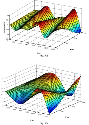
eigenvalue, depends on the type of the boundary conditions applied at the lateral edges. Specifically, the staggered order for nodes and antinodes, which is observed in the modes obtained in the free vibration problem (Holdsworth and Glynn, 1978), likewise, can be obtained in the full model wherein the pressure perturbations are applied at the lateral edges (Fig. 5). If the pressure perturbations are expressed as

25

P′=P′0cos(kx+α), the ice-shelf deflection takes the shape (for some peaks), when

(12)

TCD

8, 6059–6078, 2014

model

Y. V. Konovalov

Title Page

Tables Figures

◭ ◮

Back Close

Full Screen / Esc

Discussion

P

a

per

|

Discussion

P

a

per

|

Discussion

P

a

per

|

Discussion

P

a

per

|

is described asP′=P′0cos(ωt+kx+α), thus, the boundary condition ∂P

′

∂n =0 at the

lateral edges was considered as the basic.

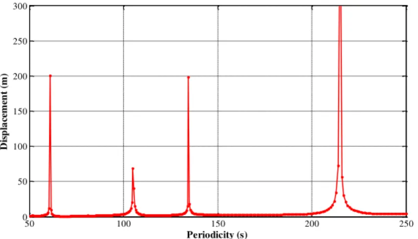
The observations on the Ross Ice Shelf have shown that more significant mechani-cal impacts on the Ross Ice Shelf result from the infragravity waves with periods from about 50 to 250 s (Bromirski et al., 2010). These waves are generated along

continen-5

tal coastlines by nonlinear wave interactions of storm-forced shoreward propagating swells (Bromirski et al., 2010). The model developed here reveals five distinct reso-nance peaks in the infragravity part of the spectrum (Fig. 6). The results of the mod-elling prove the conjecture about the possible resonant impact of the infragravity waves to the Antarctic ice-shelves.

10

Thus, the full 3-D model yields to qualitatively same results, which were obtained in the model based on the thin-plate approximation (Holdsworth and Glynn, 1978). In addition, the full model allows to observe 3-D effects, for instance, vertical distri-bution of the stress components. In particular, the full model reveals the increasing in shear stress, which is neglected in the thin-plate approximation, from the terminus

15

towards the grounding zone with the maximum at the grounding line in the case of high-frequency forcing.

References

Bassis, J. N., Fricker, H. A., Coleman, R., and Minster, J.-B.: An investigation into the forces that drive ice-shelf rift propagation on the Amery Ice Shelf, East Antarcyica, J. Glaciol., 54, 20

17–27, 2008.

Blatter, H.: Velocity and stress fields in grounded glaciers: a simple algorithm for including deviatoric stress gradients, J. Glaciol., 41, 333–344, 1995.

Bromirski, P. D., Sergienko, O. V., and MacAyeal, D. R.: Transoceanic infragravity waves im-pacting Antarctic ice shelves, Geophys. Res. Lett., 37, L02502, doi:10.1029/2009GL041488, 25

2009.

(13)

TCD

8, 6059–6078, 2014

model

Y. V. Konovalov

Title Page

Tables Figures

◭ ◮

Back Close

Full Screen / Esc

Discussion

P

a

per

|

Discussion

P

a

per

|

Discussion

P

a

per

|

Discussion

P

a

per

|

Gudmundsson, G. H.: Ice-stream response to ocean tides and the form of the basal sliding law, The Cryosphere, 5, 259–270, doi:10.5194/tc-5-259-2011, 2011.

Hindmarsh, R. C. A. and Hutter, K.: Numerical fixed domain mapping solution of free surface flows coupled with an evolving interior field, Int. J. Numer. Anal. Met., 12, 437–459, 1988. Hindmarsh, R. C. A. and Payne, A. J.: Time-step limits for stable solutions of the ice sheet 5

equation, Ann. Glaciol., 23, 74–85, 1996.

Holdsworth, G. and Glynn, J.: Iceberg calving from floating glaciers by a vibrating mechanism, Nature, 274, 464–466, 1978.

Konovalov, Y. V.: Inversion for basal friction coefficients with a two-dimensional flow line model using Tikhonov regularization, Res. Geophys., 2, 82–89, 2012.

10

Konovalov, Y. V.: Ice-shelf resonance deflections modelled with a 2D elastic centre-line model, Phys. Rev. Res. Int., 4, 9–29, 2014.

Lamb, H.: Hydrodynamics, 6th Edn., Cambridge University Press, 1994.

Landau, L. D. and Lifshitz, E. M.: Theory of Elasticity, Course of Theoretical Physics, Vol. 7, 3rd Edn., Butterworth-Heinemann, Oxford, 1986.

15

Lurie, A. I.: Theory of Elasticity, Springer, Berlin, 2005.

MacAyeal, D. R., Okal, E. A., Aster, R. C., Bassis, J. N., Brunt, K. M., Cathles, L. M., Drucker, R., Fricker, H. A., Kim, Y.-J., Martin, S., Okal, M. H., Sergienko, O. V., Spon-sler, M. P., and Thom, J. E.: Transoceanic wave propagation links iceberg calving margins of Antarctica with storms in tropics and Northern Hemisphere, Geophys. Res. Lett., 33, L17502, 20

doi:10.1029/2006GL027235, 2006.

Meylan, M., Squire, V. A., and Fox, C.: Towards realism in modelling ocean wave behavior in marginal ice zones, J. Geophys. Res., 102, 22981–22991, 1997.

Pattyn, F.: A new three-dimensional higher-order thermomechanical ice sheet model: basic sensitivity, ice stream development, and ice flow across subglacial lakes, J. Geophys. Res., 25

108, 2382, doi:10.1029/2002JB002329, 2003.

Reeh, N., Christensen, E. L., Mayer, C., and Olesen, O. B.: Tidal bending of glaciers: a linear viscoelastic approach, Ann. Glaciol., 37, 83–89, 2003.

Rosier, S. H. R., Gudmundsson, G. H., and Green, J. A. M.: Insights into ice stream dy-namics through modelling their response to tidal forcing, The Cryosphere, 8, 1763–1775, 30

doi:10.5194/tc-8-1763-2014, 2014.

(14)

TCD

8, 6059–6078, 2014

model

Y. V. Konovalov

Title Page

Tables Figures

◭ ◮

Back Close

Full Screen / Esc

Discussion

P

a

per

|

Discussion

P

a

per

|

Discussion

P

a

per

|

Discussion

P

a

per

|

Sergienko, O. V.: Elastic response of floating glacier ice to impact of long-period ocean waves, J. Geophys. Res., 115, F04028, doi:10.1029/2010JF001721, 2010.

Squire, V. A., Dugan, J. P., Wadhams, P., Rottier, P. J., and Liu, A. K.: Of ocean waves and sea ice, Annu. Rev. Fluid Mech., 27, 115–168, 1995.

Turcotte, D. L. and Schubert, G.: Geodynamics, 3rd Edn., Cambridge University Press, Cam-5

bridge, 2002.

Vaughan, D. G.: Tidal flexure at ice shelf margins, J. Geophys. Res., 100, 6213–6224, 2002. Wadhams, P.: The seasonal ice zone, in: Geophysics of Sea Ice, edited by: Untersteiner, N.,

(15)

TCD

8, 6059–6078, 2014

model

Y. V. Konovalov

Title Page

Tables Figures

◭ ◮

Back Close

Full Screen / Esc

Discussion

P

a

per

|

Discussion

P

a

per

|

Discussion

P

a

per

|

Discussion

P

a

per

|

Fig. 1,a

Fig. 1,b

Fig. 1,c

–

shelf “rolled” surface (sinusoidally perturbed – “bumpy” sea bed

0 2000 4000 6000 8000 10000 12000 14000 -350

-300 -250 -200 -150 -100 -50 0 50

Distance from the grounding line (X, m)

E

le

v

a

ti

o

n

(

m

)

Ice Shelf Surface Ice Shelf Base Sea Bottom

0 2000 4000 6000 8000 10000 12000 14000 0 500

1000 1500

0 10 20 30 40

Y (m) X (m)

E

le

v

a

ti

o

n

(

m

)

0 2000

4000 6000 8000

1000012000 14000

0 500 1000 1500

-380 -360 -340 -320 -300 -280

X (m) Y (m)

E

le

v

a

ti

o

n

(

m

)

(16)

TCD

8, 6059–6078, 2014

model

Y. V. Konovalov

Title Page

Tables Figures

◭ ◮

Back Close

Full Screen / Esc

Discussion

P

a

per

|

Discussion

P

a

per

|

Discussion

P

a

per

|

Discussion

P

a

per

|

–

(blue color) is the amplitude spectrum obtained for “rolled” ice surface (green color) is the amplitude spectrum obtained for “bumpy”

5 10 15 20 25 30 35 40 45

0 2 4 6 8 10 12 14 16 18 20

Periodicity (s)

D

is

p

la

ce

m

en

t

(m

)

(17)

TCD

8, 6059–6078, 2014

model

Y. V. Konovalov

Title Page

Tables Figures

◭ ◮

Back Close

Full Screen / Esc

Discussion

P

a

per

|

Discussion

P

a

per

|

Discussion

P

a

per

|

Discussion

P

a

per

|

Fig. 3,a

Fig. 3,b

Fig. 3,c



33 



0 2000 4000 6000 8000 10000 12000 14000 0

500 1000

1500

-0.5 0 0.5 1

Y (m) X (m)

D

is

p

la

ce

m

en

t

(m

)

0 2000 4000 6000 8000 10000 12000 14000 0

500 1000

1500

-0.5 0 0.5 1 1.5

Y (m) X (m)

D

is

p

la

ce

m

en

t

(m

)

0 ₂₀₀₀ 4000 ₆₀₀₀

8000 ₁₀₀₀₀

12000 ₁₄₀₀₀ 0 500

1000 1500 -3

-2 -1 0 1 2

Y (m) X (m)

D

is

p

la

ce

m

en

t

(m

)

Figure 3.Ice-shelf deflections obtained for the three modes:(a)period is equal to 14.9 s;(b) pe-riod is equal to 19.7 s;(c)period is equal to 27.1 s. Young’s modulusE=9 GPa, Poisson’s ratio

(18)

TCD

8, 6059–6078, 2014

model

Y. V. Konovalov

Title Page

Tables Figures

◭ ◮

Back Close

Full Screen / Esc

Discussion

P

a

per

|

Discussion

P

a

per

|

Discussion

P

a

per

|

Discussion

P

a

per

|

Fig. 4,a

Fig. 4,b

 

Distance from the Grounding Line (m)

E

le

v

at

io

n

(

m

)

0 2000 4000 6000 8000 10000 12000 14000

-300 -250 -200 -150 -100 -50 0

-2 -1.5 -1 -0.5 0 0.5 1 1.5 x 106

(Pa)

Distance from the Grounding Line (m)

E

le

v

a

ti

o

n

(

m

)

0 2000 4000 6000 8000 10000 12000 14000

-300 -250 -200 -150 -100 -50 0

-7 -6 -5 -4 -3 -2 -1 0 1 x 105

(Pa)

(19)

TCD

8, 6059–6078, 2014

model

Y. V. Konovalov

Title Page

Tables Figures

◭ ◮

Back Close

Full Screen / Esc

Discussion

P

a

per

|

Discussion

P

a

per

|

Discussion

P

a

per

|

Discussion

P

a

per

|

Fig. 5,a

Fig. 5,b

    

  33

0 2000

4000 6000

8000 10000

12000 14000 0

500 1000

1500

-1.5 -1 -0.5 0 0.5 1

Y (m)

X (m)

D

is

p

la

ce

m

en

t

(m

)

0 2000

4000 6000

8000 10000

12000 14000 0

500 1000

1500 -2

-1.5 -1 -0.5 0 0.5 1 1.5 2

Y (m) X (m)

D

is

p

la

ce

m

en

t

(m

)

(20)

TCD

8, 6059–6078, 2014

model

Y. V. Konovalov

Title Page

Tables Figures

◭ ◮

Back Close

Full Screen / Esc

Discussion

P

a

per

|

Discussion

P

a

per

|

Discussion

P

a

per

|

Discussion

P

a

per

|

50 100 150 200 250

0 50 100 150 200 250 300

Periodicity (s)

D

is

p

la

ce

m

en

t

(m

)