www.atmos-chem-phys.net/13/1941/2013/ doi:10.5194/acp-13-1941-2013
© Author(s) 2013. CC Attribution 3.0 License.
Atmospheric
Chemistry
and Physics
Geoscientific
Geoscientific
Geoscientific
Geoscientific
Environmental impacts of shipping in 2030 with a particular focus
on the Arctic region
S. B. Dalsøren1, B. H. Samset1, G. Myhre1, J. J. Corbett2, R. Minjares3, D. Lack4,5, and J. S. Fuglestvedt1 1CICERO, Center for International Climate and Environmental Research Oslo, Norway
2College of Earth, Ocean, and Atmosphere, University of Delaware, Newark, USA 3The International Council on Clean Transportation, San Francisco, USA
4NOAA Earth System Research Laboratory, Chemical Sciences Division, Boulder, USA
5Cooperative Institute for Research in Environmental Sciences, University of Colorado, Boulder, USA
Correspondence to: S. B. Dalsøren ([email protected])
Received: 13 July 2012 – Published in Atmos. Chem. Phys. Discuss.: 9 October 2012 Revised: 25 January 2013 – Accepted: 6 February 2013 – Published: 20 February 2013
Abstract. We quantify the concentrations changes and Ra-diative Forcing (RF) of short-lived atmospheric pollutants due to shipping emissions of NOx, SOx, CO, NMVOCs, BC and OC. We use high resolution ship emission inventories for the Arctic that are more suitable for regional scale eval-uation than those used in former studies. A chemical trans-port model and a RF model are used to evaluate the time period 2004–2030, when we expect increasing traffic in the Arctic region. Two datasets for ship emissions are used that characterize the potential impact from shipping and the de-gree to which shipping controls may mitigate impacts: a high (HIGH) scenario and a low scenario with Maximum Feasible Reduction (MFR) of black carbon in the Arctic. In MFR, BC emissions in the Arctic are reduced with 70 % representing a combination technology performance and/or reasonable ad-vances in single-technology performance. Both scenarios re-sult in moderate to substantial increases in concentrations of pollutants both globally and in the Arctic. Exceptions are black carbon in the MFR scenario, and sulfur species and organic carbon in both scenarios due to the future phase-in of current regulation that reduces fuel sulfur content. In the season with potential transit traffic through the Arctic in 2030 we find increased concentrations of all pollutants in large parts of the Arctic. Net global RFs from 2004–2030 of 53 mW m−2(HIGH) and 73 mW m−2(MFR) are similar to those found for preindustrial to present net global aircraft RF. The found warming contrasts with the cooling from his-torical ship emissions. The reason for this difference and the higher global forcing for the MFR scenario is mainly the
re-duced future fuel sulfur content resulting in less cooling from sulfate aerosols. The Arctic RF is largest in the HIGH sce-nario. In the HIGH scenario ozone dominates the RF during the transit season (August–October). RF due to BC in air, and snow and ice becomes significant during Arctic spring. For the HIGH scenario the net Arctic RF during spring is 5 times higher than in winter.
1 Introduction
Observations over the past 50 yr show a decline in Arctic sea-ice extent throughout the year, with fastest retreat in sum-mer (Serreze et al., 2007; Lemke et al., 2007; Stroeve et al., 2012a, b). Less sea-ice cover and reduced ice thickness im-plies improved access for shipping around the margins of the Arctic Basin. Climate models project an acceleration of the ice melting leaving the Arctic Ocean increasingly open to shipping (Meehl et al., 2007; Stroeve et al., 2012a). In the next decades melting of sea ice may open entirely new pos-sibilities with respect to new shipping routes in the Arctic (Stephenson et al., 2011; Arctic Council, 2009). Studies are examining the implications of emergent new shipping routes and extension of the period during which shipping is feasi-ble (Corbett et al., 2010a; Paxian et al., 2010; Peters et al., 2011). Unless measures are taken increases in emissions are expected (Corbett et al., 2010a).
Russia, and sea transport along the Northern Sea Route. They found significant regional effects by increases of acid de-position in the North Scandinavia and the Kola Peninsula. Augmented levels of particles over much of the Arctic were also calculated. Granier et al. (2006) studied the potential in-creases in ozone pollution using one of the upper emission estimates for 2050 from Eyring et al. (2005) and introduced a scenario where shipping activity grows with an increase in ice-free Arctic waters. During the summer months, surface ozone concentrations in the Arctic could be enhanced by a factor of 2–3 as a consequence of ship operations through the northern passages. Projected ozone concentrations from July to September were comparable to summertime values cur-rently observed in many industrialized regions in the North-ern Hemisphere.
Ship emissions are projected to increase significantly also outside Arctic waters due to increases in transportation de-mand and traffic (Eyring et al., 2005; Paxian et al., 2010; Buhaug et al., 2009; Eide, 2007). Most scenarios for the next 10–20 yr indicate that efficiency improvements and emis-sion controls due to current regulatory policies could be out-weighed by an increase in traffic resulting in a global increase in emissions. Of course, policy-induced controls are very de-pendent on the success of adapted and proposed regulations within the International Maritime Organization (IMO) and other regulatory bodies (Eyring et al., 2010; Buhaug et al., 2009). Results for future global impacts from ship emissions are therefore dependent on the projections used as baseline for the emission calculations. Cofala et al. (2007) find that the contribution from shipping to sulfur deposition in Euro-pean coastal areas is expected to increase by 2020 to more than 30 % in large areas, and up to 50 % in coastal areas. The impacts of possible near future sulfur regulations on health and climate were quantified by Lauer et al. (2009) and Wine-brake et al. (2009). Technologies exist to reduce emissions from ships beyond what is currently legally required. Cofala et al. (2007) also performed a cost-effectiveness analysis for several possible sets of measures. Eyring et al. (2007) used results from ten state-of-the-art atmospheric chemistry mod-els to analyse present-day conditions (year 2000) and two future ship emission scenarios. In one scenario ship emis-sions stabilize at 2000 levels, in the other ship emisemis-sions
studies. Section 4 is devoted to the impacts on pollution (at-mospheric composition) and climate (radiative forcing). We focus on short-lived components which we define as primary or secondary products with lifetimes shorter than the longest timescale for mixing in the troposphere, i.e. 1–2 yr for inter-hemispheric mixing. Section 5 discusses the results and treats uncertainties, while the major findings are summarized and set into a perspective in Sect. 6.
2 Emission scenarios
Corbett et al. (2010a) provides gridded inventories for cur-rent (2004) and future (2030, 2050) ship emissions of green-house gases and gas and particulate pollutants in the Arctic. That study presents several options for emission totals and diversion routes through the Arctic in 2030. In this study we compare their highest and lowest estimates to get an impres-sion of the range of possible future effects due to emisimpres-sions of NOx, SOx, CO, NMVOCs, BC and OC. Table 1a com-pares the yearly total Arctic ship emissions for some of these components, for 2004 and for our two 2030 scenarios.
In the high growth scenario (HIGH) there is more than a doubling in energy use for shipping serving the Arctic. In addition 2 % of the global traffic diverts to Arctic through-routes. Global shipping growth outside the Arctic is+3.3 % per year on average, and most uncontrolled emissions grow proportionally to shipping activity. For some pollutants there are exceptions; SOxand NOxfollow new IMO regulations to be implemented by 2020 and OC is correlated with changes in SOx emissions (Lack et al., 2009). Large emission in-creases (factors of 2 to 5) are found (Table 1a) for all species except sulfur where regulations on sulfur content outweigh the increase in fuel consumption. The emissions from di-version traffic are larger than those from the fleet operating solely within the Arctic.
Table 1a. Ship emissions north of 60◦N in 2004 and 2030
(Kton yr−1) from Corbett et al. (2010a). There is seasonal variation
in the emissions from the Arctic fleet. The diversion fleet operates in the period August–October. Numbers in bold are total emission each year, numbers in normal font are emissions for the sections of the total fleet.
NOx SO2 BC OC
2004 196 136 0.88 2.70 2030 HIGH 739 130 4.50 5.10
Arctic fleet 329 58 2.00 2.30
Diversion fleet 410 72 2.50 2.80
2030 MFR 384 68 0.76 0.84
Arctic fleet 244 43 0.46 0.51
Diversion fleet 140 25 0.30 0.33
Table 1b. Non-Arctic ship emissions in 2004 and 2030 (Kton yr−1). The non-Arctic ship traffic distribution and emissions for 2004 are from Dalsøren et al. (2009). The 2030 emission scenarios are based on Corbett et al. (2010a). There is seasonal variation in the emis-sions.
NOx SO2 BC OC
2004 15 187 8699 35 120
2030 HIGH 24 854 3672 80 97
2030 MFR 18 063 2668 58 73
performance. Technologies for reducing BC emissions are discussed briefly in Corbett et al. (2010a) and in detail in Corbett et al. (2010b). 1 % of the global traffic diverts to Arc-tic through-routes, and global shipping growth outside the Arctic is+2.1 % per year. SOx and NOxreductions follow IMO regulations and OC is correlated with SOx, unless ad-ditionally reduced by MFR controls. For the 2030 MFR sce-nario NOxemissions in the Arctic (Table 1a) are doubled, but MFR controls reduce BC by some 70 %, sulfur emissions are halved, and OC which is correlated both with sulfur and BC is about one third. With these scenario conditions, yearly to-tal emissions for regional traffic in MFR are factors 1.5 to 1.7 larger than for the diversion traffic.
Large seasonal variations described by Corbett et al. (2010a) are embedded in the yearly total Arctic shipping emissions in Table 1a. Emissions are dominated by sum-mer and fall activity. For 2004 winter (December–February) and spring (March–May) emissions are 30 % lower than the other seasons. For 2030 the seasonal differences are even larger due to the diversion traffic operating only in 3 months (August–October). Following the recommendations from Corbett et al. (2010a) Table 12, we assume that traffic in 2030 in diversion routes follows the coasts, passing through the Northeast Passage and Northwest Passage. We have not imposed traffic over the pole as that route may not become available until after 2050 (Corbett et al., 2010a).
In order to get global gridded ship emissions we com-plement the Arctic inventories from Corbett et al. (2010a) with those for 2004 from Dalsøren et al. (2009). The Arc-tic inventory covers the AMAP region and the Dalsøren et al. (2009) dataset elsewhere. For definition of the AMAP re-gion see Peters et al. (2011). This definition is used to easily compare this study with the results from a separate ongo-ing study (Dalsøren et al., 2013) usongo-ing the 2030 and 2050 Arctic ship emissions from Peters et al. (2011). For the non-Arctic developments from 2004 to 2030 are obtained assum-ing changes in emission totals in accordance with Corbett et al. (2010a) (+3.3 % per year in HIGH,+2.1 % per year in MFR). The non-Arctic ship emissions are shown in Table 1b. As in the Arctic scenarios, SOxand NOx follow IMO reg-ulations, while OC is correlated with changes in SOx emis-sions. Uniform scaling is used from 2004 to 2030 assuming no changes of the trade routes outside the Arctic.
For all model simulations we used the Edgar 3.2 inventory (Olivier et al., 2005) for non-ship anthropogenic emissions and the RETRO inventory (Schultz et al., 2007) for natural emissions. No changes were made in these emissions be-tween the model simulations for 2004 and 2030.
3 Model and methods
To calculate the impacts on pollution and chemical composi-tion the OsloCTM2 model was used. Simulacomposi-tions were per-formed in T42 resolution (2.8◦×2.8◦) with 60 vertical layers
using meteorological data for 2006. The tropospheric dis-tributions of 137 chemical species are calculated, amongst them hydrogen, oxygen, nitrogen, and carbon containing gases and also sulfate, nitrate, primary organic, secondary organic, black carbon (BC), and sea salt aerosols. The gas and aerosol schemes are described in (Myhre et al., 2009; Skeie et al., 2011a, b; Berglen et al., 2004; Ødemark et al., 2012; Hoyle et al., 2007). OsloCTM2 modeled distributions of ozone and ozone precursors in coastal regions were eval-uated and compared to observations in some former ship im-pact studies (Endresen et al., 2003; Dalsøren et al., 2007, 2010). The model results corresponded with those of other models in a model assessment of ship impact (Eyring et al., 2007). A basis simulation was performed for 2004 and then runs were done with the 2030 HIGH and MFR ship emission scenarios. Meteorology and emissions from all other sectors were kept identical in the three simulations. All simulations had 5 months of spin-up starting with the same initial condi-tions.
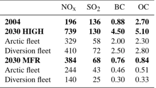
Fig. 1. NO2 in the lowest model layer close to the surface (pptv). (A) Average 2004 for the months August-September-October (ASO).
(B) Average change 2004–2030 for HIGH scenario for the months November-December-January (NDJ). (C) Same as (B), MFR scenario,
months ASO. (D) Same as (B), HIGH scenario, months ASO.
thermal infrared scheme is also implemented (Myhre et al., 2011). Temporal and spatial resolutions were the same as for OsloCTM2 for aerosols, whereas monthly mean data were used for ozone. The optical properties of aerosols in the model are discussed in Myhre et al. (2007). Direct radiative forcing was calculated as the difference in top-of-atmosphere energy flux between a simulation with all components at 2030 levels, and one that has one component changed to 2004 levels. Stratospheric temperature adjustment was included in the calculations for ozone changes. Standard backgrounds of other aerosols were always present in the calculations. A similar scheme was used for calculating the effects of BC deposition on snow (Skeie et al., 2011a). The first indirect aerosol (cloud albedo) effect was calculated by estimating cloud droplet number from an empirical relationship with aerosol concentration (Quaas and Boucher, 2005; Quaas et al., 2006), and calculating the difference between aerosols at 2030 and 2004 levels as for the direct aerosol effect. See Ødemark et al. (2012) for details.
4 Results
To illustrate the large dependency of atmospheric impacts on seasonality in emissions and meteorology results are shown as seasonal means. Averages are made for the four sea-sons NDJ (November-December-January), FMA (February-March-April), MJJ (May-June-July) and ASO
(August-September-October, i.e., the period with Arctic transit traffic in 2030).
4.1 Changes in pollution and chemical composition
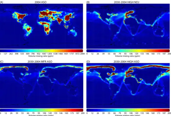
Fig. 2. O3in the lowest model layer close to the surface (ppbv). Averages 2004 for the months November-December-January (NDJ) (A) and August-September-October (ASO) (B). Average change 2004–2030 MFR scenario for the months NDJ (C) and ASO (D). Average Change 2004–2030 HIGH scenario for the months NDJ (E) and ASO (F).
The year 2004 ASO and NDJ distributions of surface ozone are shown in Fig. 2. High levels are found down-wind of polluted regions with extended periods of sunlight and favorable conditions for ozone formation, especially over oceans and deserts where dry deposition is slow. The changes in the MFR scenario are moderate, a few ppbv/percent over the oceans and coastal areas. Except for the ASO season small changes are found in the Arctic region. This is ex-pected since the NOxemissions from traffic within the Arc-tic are only slightly larger than in 2004. Since ship emis-sions of other ozone precursors (VOCs, CO) are small, NOx (NO+NO2)is decisive for ozone generation from shipping (Endresen et al., 2003). For the MFR in the ASO season the effect of diversion traffic on ozone is limited since it occurs (August–October) outside the months with maximum inso-lation. In September–October the sunlight in the Arctic is rapidly diminishing and ozone formation is getting less
ef-ficient. In general substantial increases of 2 to above 5 ppv (4 to above 10 %) are found in the Northern Hemisphere coastal and oceanic regions for the HIGH scenario. Many of the countries in western Europe see ozone increases on the order 3–6 %. In pristine regions of the tropical and Arctic Oceans the increases are above 10 %. In MJJ (not shown) the magnitude and spatial patterns of changes has many similar-ities to ASO. However, the changes in the Arctic are smaller since diversion traffic is absent, and larger over oceanic areas 30–60◦N due to the maximum in photochemical activity.
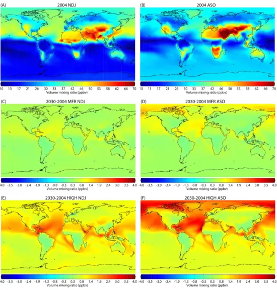
Fig. 3. Sulfate in the lowest model layer close to the surface (pptv). (A) Average 2004 for the months August-September-October (ASO). (B)
Average change 2004–2030 HIGH scenario for the months ASO. (C) Same as (B), MFR scenario (D) Same as (B), HIGH scenario, months November-December-January (NDJ).
than the decrease of sulfur emissions. This is because most sulfur is emitted as SO2, and increases in oxidants (OH, O3 and H2O2)lead to more efficient sulfate formation. On the west coast of the continents with prevailing westerly winds, a reduction of around 50 pptv or 10–15 % is clearly of signif-icance, both with regard to health impact from particle pol-lution and acid precipitation. Effects of future sulfur regu-lations on particulate matter concentrations and mortality is discussed in detail in Lauer et al. (2009) and Winebrake et al. (2009). An increase of up to 50 % is found for the ASO season for the HIGH scenario in proximity to the new di-version routes. This is expected as there are few other large sources of sulfur emissions close to these routes.
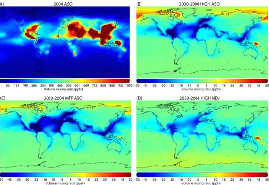
The highest surface concentrations of black carbon (BC) are found in China and India where biofuel use in house-holds is common (Fig. 4). High levels are also found in other densely populated regions, megacities and areas with vegeta-tion burning. Outside the Arctic future shipping leads to in-creased BC in the vicinity of major shipping routes. Typical increases are 3–20 ng m−3(10–20 %) for the HIGH case, and somewhat lower for the MFR scenario. The largest absolute perturbations are found in the North Sea and other regions with much traffic. However, the largest relative increases are found in the less trafficked area near Antarctica due to the very low background values there. For the MFR scenario in the ASO season the Arctic has a decrease of about 10 % in regions with internal traffic, and a similar or larger increase in the regions with diversion traffic. For the HIGH scenario,
which has no measures on BC emissions, the situation is dif-ferent. There is an increase in the whole of Arctic (Fig. 4), and the signals along the diversion routes are very evident. The BC levels increase more than 50 % in much of the Arc-tic. Arctic changes are smallest in NDJ in both scenarios, mainly due to less traffic and emissions in winter.
The surface distribution of OC (Fig. 5) for 2004 shows many of the same source signatures as BC, but with a stronger signal around regions with vegetation fires. From 2004–2030 OC concentrations due to shipping decline in most regions, since OC emissions are correlated with SOx emissions and sulfur content is reduced following IMO regu-lations. Reductions are typically 4–20 ng m−3near shipping lanes in the MFR case. This corresponds to a relative reduc-tion of about 5 % both at mid- and polar latitudes. The diver-sion routes in the ASO season are again an exception, with increases of 10–30 % in the HIGH scenario.
4.2 Global Radiative Forcing (RF)
Fig. 4. Same as Fig. 3 for BC (ng m−3).
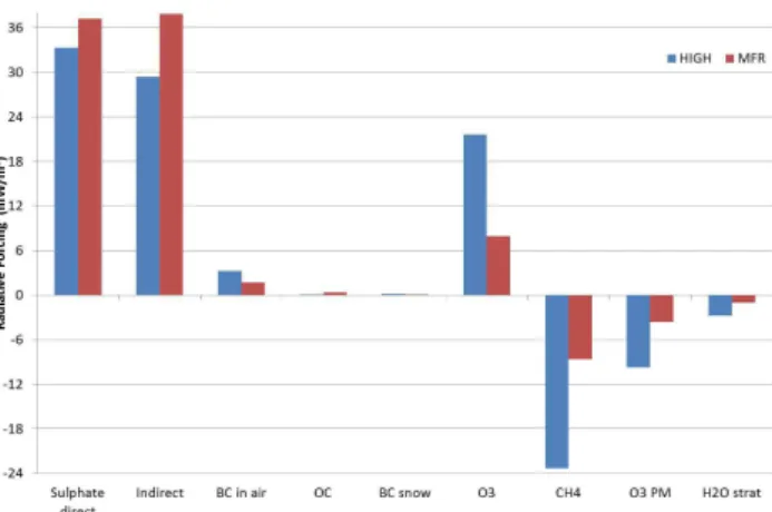
Fig. 6. Global RF (mW m−2)from 2004–2030 per component for the scenarios HIGH and MFR.
also the dominant cause of the indirect aerosol effect. The magnitudes of the direct sulfate and indirect aerosol effects are quite similar. Due to the strong reductions of sulfur emis-sions there are small differences in RF between the two sce-narios. Interestingly, the difference is larger for the indirect effect than for the direct. We found that the normalized RFs with respect to burden are quite similar for the direct effects, and that there are nonlinearities from concentration changes to RF for the indirect effect. Sensitivity studies also suggest a logarithmic relation between emissions and the indirect ef-fect (Lund et al., 2012). Ozone chemistry can also be non-linear in regions with high background NOx levels. How-ever, most shipping regions are relatively remote or mod-erately polluted and have shown quite linear responses in earlier studies (Eyring et al., 2007). The main cause of the difference of almost factor three in ozone RF between the two scenarios is therefore the span in NOx emissions (Ta-ble 1b) rather than non-linearity. The RF signal from ozone in the HIGH scenario is almost as large as those from the indirect aerosol and direct sulfur effects. Ship emissions of methane are small and the direct radiative effects from these are negligible. Due to the relatively high NOx and low CO and NMVOCs emissions, shipping efficiently increases OH and thereby decreases methane lifetime by increasing the chemical loss. Methane changes in turn leads to changes in ozone, called Primary Mode (PM) ozone, and stratospheric water vapour. We therefore included simplified calculations of methane RF, even if methane is seldom defined as a short-lived climate forcer. We used the approach described in Berntsen et al. (2005) and Myhre et al. (2011) to calculate the global radiative forcings from methane and associated ozone and stratospheric water vapor changes. The RF values from this method apply for the time when the perturbations have reached equilibrium conditions. As in other shipping stud-ies (Eyring et al., 2010) we find that the associated methane RF more than outweighs the positive RF from ozone changes
Fig. 7. Net global RF (mW m−2)from 2004–2030 for different sea-sons for the scenarios HIGH and MFR.
(Fig. 6). The contribution from BC and OC to global total RF is small, and nitrate RF is negligible.
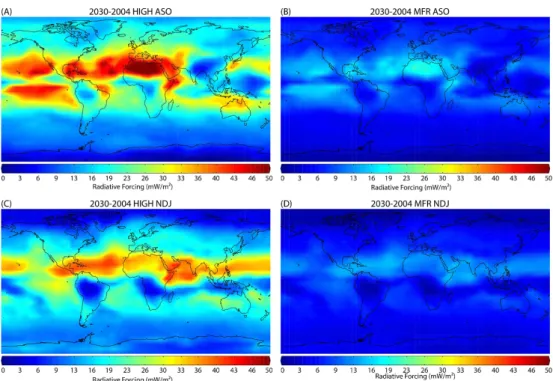
The seasonality in global net 2004–2030 RF from ships is shown in Fig. 7. Seasonal differences are up to a factor 1.5. For the strongly scattering components (sulfate and OC) the magnitude of the RF is largest in the MJJ season, the sea-son with largest insolation, in the regions of Northern Hemi-sphere where most ship emissions occur. Interestingly, the global RF for ozone is larger for the ASO season (Fig. 8) than the MJJ (not shown) even if one would expect photo-chemical activity in the Northern Hemisphere to be stronger in MJJ. BC RF is also higher for ASO. Global total ship emis-sions are slightly higher in ASO than MJJ, but this is likely not the main cause. As shown in Figs. 8 and 9 the strongest ozone and BC in air forcing is found over the region 20– 30◦N over Sahara and areas with low frequency of clouds
(ozone) or high albedo (BC). The increase in column loading (not shown) in this area is larger for ASO. The difference is probably caused by the position and movement of the Inter Tropical Convergence Zone (ITCZ) resulting in less wet re-moval and stronger vertical transport of ozone precursors and BC in ASO. The RF for ozone is largest in the vicinity of the subtropical jets where ozone lifetime is long and ozone for-mation from precursors efficient. Even if the seasons of NDJ and ASO show quite different geographical signal for surface ozone changes (Fig. 2) the RF maps for these seasons (Fig. 8) are quite similar.
Fig. 8. Ozone RF 2004–2030 (mW m−2). (A) HIGH scenario, ASO season. (B) MFR scenario, ASO season. (C) HIGH scenario, NDJ season. (D) MFR scenario, NDJ season.
Fig. 9. BC in air RF 2004–2030 (mW m−2)for the ASO season. (A) MFR scenario. (B) HIGH scenario.
coincidence between high emissions and low level marine clouds is a decisive prerequisite.
For all species the RF is largest for the ship scenario with largest changes in emissions. With most components having a positive RF the overall result from 2004 to 2030 is a warm-ing. Due to the important role of sulfur, the MFR scenario gives larger global mean total forcing than HIGH since it has the largest reduction in emissions. The global RFs for ozone and methane for the HIGH scenario are of comparable mag-nitude to RF from international shipping from pre-industrial to 2000 in studies with this model (Myhre et al., 2011; En-dresen et al., 2003) as well as other models (Myhre et al., 2011; Eyring et al., 2010). Comparing with historical aerosol climate impacts (Eyring et al., 2010; Balkanski et al., 2010) the RFs from 2004–2030 (MFR and HIGH) are of similar
Fig. 10. Yearly mean sulfate direct RF 2004–2030 (mW m−2)for the MFR scenario (A) and HIGH scenario (B). Yearly mean first indirect
aerosol RF 2004–2030 (mW m−2)for the MFR scenario (C) and HIGH scenario (D).
Fig. 11. RF 2004–2030 (mW m−2)in the Arctic (60–90◦N) for
dif-ferent seasons and components for the scenarios HIGH and MFR.
N2O is not accounted for in these numbers. These values are very similar to the numbers reported for historic aircraft RF in 2005, 55 mW m−2 or 78 mW m−2including cirrus cloud enhancement (Lee et al., 2010).
4.3 Arctic Radiative Forcing (RF)
Figure 11 shows the RF per component, seasonally averaged over 60–90◦N. In the Arctic the indirect aerosol effect is
weaker than the direct sulfate RF due to less efficient cloud
formation. The indirect effect is weak except for the MJJ sea-son. It turns negative in the ASO HIGH case due to extensive sulfate increase in the Arctic connected with diversion traf-fic (also the case for OC RF). For MFR the direct sulfate effect is strongest with the indirect aerosol effect and ozone RF about equal as second most important. For the HIGH case ozone RF is strongest, and stronger than the direct sulfate RF except for the MJJ season. During the period with transit traf-fic (ASO) the ozone RF is more than double that of forcing from any other component in the HIGH case. BC forcing is of more significance in the Arctic than for the global mean. In the HIGH scenario the RF for BC on snow/ice in MJJ is large since this is the season with onset of snowmelt and BC has accumulated in snow throughout the winter. Averaged over the seasons the RF from BC in air and BC on snow/ice is approximately 60 % lower for the Maximum Feasible Re-duction (MFR) scenario. The RF from OC is almost negligi-ble for both scenarios. Similar to Ødemark et al. (2012) we find the RF from nitrate to be negligible. There are large sea-sonal differences also when the Arctic RF is summed up for all components. The total RF is more than a factor 5 larger in the MJJ season than in the NDJ season. The factor is around 3 comparing MJJ and FMA.
5 Discussion
The ship emission scenarios used in this study are based on the state of understanding at the time the emission stud-ies (Corbett et al., 2010a; Dalsøren et al., 2009) were per-formed. The development of NOx therefore follows global IMO regulations to be implemented by 2020 but does not include recently adopted regional Emission Control Areas (ECAs) that have more stringent standards. Recent findings also suggest that emissions of BC, particularly in the Arc-tic, will be very dependent on fuel type, speed and vessel type (Lack and Corbett, 2012). The emission factors used in the Dalsøren et al. (2009) and Corbett et al. (2010a) datasets forming the basis for the scenarios are similar, except for higher values for BC and OC in the Arctic inventory (Corbett et al., 2010a) taking into account recent findings by Lack et al. (2009). We might therefore underestimate the impact of BC and OC shipping emissions outside Arctic waters. How-ever, this should not impact our conclusions since their im-pact is rather small compared to the signal from other compo-nents (e.g. Fig. 6). The organic matter (OM) emission factor used is an average from about 100 ship plume measurements and reports the OM after the semi-volatiles have either evap-orated or condensed. Any formation of secondary species, and associated uncertainty is therefore linked to the VOC in-ventory and secondary organic aerosol (SOA) formation pro-cesses. The SOA scheme implemented in OsloCTM2 also shows small SOA values over the Arctic region (Hoyle et al., 2007). For these reasons only primary OC was included in the simulations.
Another uncertainty is the discontinuity at the overlap be-tween the grid used for Arctic ship emissions (Corbett et al., 2010a) and the global traffic grid (Dalsøren et al., 2009) representing ship emissions for the rest of the globe. The inconsistency is unavoidable as the dataset from Corbett et al. (2010a) lacks global coverage. The result is too sharp or unrealistic concentrations gradients between the Arctic and mid latitudes close to shipping lanes for some primary pol-lutants. However, the effects are small on larger scales and therefore have little influence on our main findings. We as-sumed uniform changes in ship emissions 2004–2030 out-side the Arctic region. Though international shipping is a global market with intercontinental transport, differences in regional development and new trade routes are likely. How-ever, no studies currently address these aspects outside the Arctic.
In this study there were no changes from 2004 to 2030 in non-shipping emissions. This was done to be able to easily discern the impacts from changes in ship emissions. Dalsøren et al. (2007) found that the impact of shipping on ozone was quite independent of changes in emissions from other sectors in the period 2000–2015.
Eyring et al. (2007) performed multi-model calculations for ship emissions in 2030. One of the scenarios assumed a 2.2 % annual growth from 2000 which is quite similar to the
MFR scenario. However, the results for MFR found here are not very well suited for comparison, as the assumed emis-sion distributions are very different. The Eyring et al. (2007) study used a dataset only accounting for a few of the ma-jor trade routes. Granier et al. (2006) finds much larger in-creases in ozone and NOx along diversion routes than this study. The reasons for the differences are probably related to higher emissions in 2050, 0.65 and 1.3 Tg (N) respec-tively, compared to 0.12 Tg (N) in the HIGH case in 2030 in this study. Granier et al. (2006) also introduces the traffic one month earlier (July) and Arctic ship emissions are ab-sent in their basis simulation whereas this study uses year 2004 emissions as basis. These factors would make ozone production more efficient in the Granier et al. (2006) study.
Changes in sea ice were not accounted for in the calcula-tions. This might influence dry deposition and surface albedo and thereby the chemical composition and RF calculations. However, the new Arctic routes operate close to the coast and it is likely that ice-breakers will still be needed in 2030 (Pe-ters et al., 2011). Scenarios for 2030 do not necessarily im-ply large changes in ice-extent. Taking into account changes in ice conditions on RF calculations are studied in Dalsøren et al. (2013) and found to have minor effects on RF from Arctic shipping. Identical atmospheric meteorology was used in the 2004 and 2030 simulations. Climate change towards 2030 makes changes in meteorological factors likely. Such changes were unaccounted for in this study.
The main reason that the Arctic temperatures currently rise twice as much as in the rest of the world is an amplification process involving snow, ice and albedo changes of the surface (Serreze and Barry, 2011). Increases in RF result in enhanced melting, and land or open water replace snow and ice. Both land and open water are, on average, less reflective than ice or snow, and thus absorb more solar radiation. This causes more warming which in turn may cause more melting. The pro-nounced seasonality of the RF signal is therefore interesting. We find a clear maximum of Arctic RF in MJJ which coin-cides with the melting season many places in the Arctic. The RFs for this season are 68 mW m−2 for the HIGH scenario and 45 mW m−2for the MFR scenario. This is quite similar to the values reported in Sect. 4.2 for the global yearly mean RF. Through a comparison with global historical RF it was noted in Sect. 4.2 that these magnitudes are of significance.
(Ødemark et al., 2012) due to inefficient formation of OH and low temperatures. Several oceanic regions are decided or considered as ECA (Emission Control Areas) for NOx. Though the ECAs are mainly set to limit air pollution, the Arctic could be a candidate as an ECA from a climate per-spective. A sensitivity study revealed that 2/3 of the calcu-lated ozone increase in the HIGH scenario was due to emis-sion within the region (60–90◦N), the rest was due to
trans-port from lower latitudes. It should however be noted that this study might overestimate the concentration change and RF of ozone due to the coarse resolution in the simulations with the OsloCTM2 model. Not resolving the scales of the chem-ical and physchem-ical processes in the exhaust plumes might lead to prediction of too high ozone production per emitted NOx molecule (Paoli et al., 2011). The effect of an Arctic ECA would be less if plume chemistry reduces ozone production efficiency in the Arctic similar to what studies indicate for low latitudes.
The interpretation of how the Arctic RF from a particular component affects Arctic and global temperatures is subject to some uncertainty. It is not necessarily the case that a posi-tive RF implies a regional temperature increase. Shindell and Faluvegi (2009), Sand et al. (2013) and Flanner (2013) found that positive RF for some atmospheric species in the Arctic could result in cooling in the region due to complex atmo-spheric circulation changes. More studies on these issues are needed, involving separate emission sectors and the whole cause effect chain from emissions to temperature change.
6 Conclusions
In this study we compare environmental and climate impacts, in terms of surface concentrations and RF, of high and low es-timates for ship emissions in 2030. Impacts in the Arctic are the main focus. In the high growth scenario (HIGH) there is a large increase in ship traffic within the Arctic. In addi-tion 2 % of the yearly global traffic diverts to Arctic through-routes during late summer. Global shipping growth outside the Arctic is+3.3 % per year. In the Maximum Feasible Re-duction (MFR) scenario a business as usual scenario is fol-lowed but maximum feasible reduction is applied on Arctic
lanes. Increases from 2004 to 2030 are typically in the range 10 % to above 60 % in coastal regions of the Northern Hemi-sphere, Arctic shipping regions, and main oceans shipping lanes in both hemispheres. In late summer, when operation takes place along the diversion routes, increases are above 200 % in pristine regions of the Arctic. The largest NO2 changes are found for the HIGH scenario. For surface ozone the HIGH scenario shows substantial increases of 2 to above 5 ppv (4 to above 10 %) in coastal and oceanic regions of the Northern Hemisphere. In pristine regions of the tropical and Arctic Oceans the increases are above 10 %. The changes in the MFR scenario are moderate and a few ppbv/percent over the oceans and coastal areas. The ozone RF has a quite dif-ferent geographical distribution than surface ozone. Largest 2004–2030 ozone RF is found near the subtropical jets and results from a combination of more efficient vertical trans-port and ozone formation, and low cloud cover. The largest absolute surface BC increases are found in the North Sea and other regions with much traffic. In late summer the MFR sce-nario has a decrease of about 10 % in Arctic regions with in-ternal traffic, and a similar or larger increase in the regions with diversion traffic. For the HIGH scenario the BC levels increase more than 50 % in much of the Arctic in late sum-mer. Like ozone, maximum RF from BC in air occurs at low latitudes. The strongest RF is found over Sahara due to high surface albedo and strong solar radiation.
Sulfate has the largest contribution to the global yearly mean forcing. Though, in the HIGH scenario the ozone RF is almost as large as those from the indirect aerosol and di-rect sulfur effects. Simplified calculations show that methane and associated RF are of about similar magnitude but oppo-site sign to the ozone RF for both scenarios. The contribution from BC, OC and nitrate to global RF is small. With sulfur reductions most components have a positive RF and the over-all result from 2004 to 2030 is a warming, in contrast to the historical net RF from shipping which is negative. For sev-eral components the RFs from 2004–2030 in this study are of comparable absolute magnitude to the RF from international shipping from pre-industrial to 2000, as found in studies with this or other models. The MFR scenario gives larger global mean net forcing since it has the largest reduction in sulfur emissions. The yearly average global net RFs for the short-lived climate forcers are 73 mW m−2 for the MFR scenario and 53 mW m−2 for the HIGH scenario. The positive RFs from N2O and CO2are not included in these numbers. The shipping RF from 2004–2030 is about equal to the historic aircraft RF up to 2005 (55 mW m−2or 78 mW m−2 includ-ing cirrus cloud enhancement, Lee et al., 2010).
Very large seasonal variations (up to a factor of 10) are found for Arctic RF. The indirect effect is small except for the spring season. It turns negative for a few months in the HIGH case due to extensive sulfate increase connected with diver-sion traffic (also the case for OC RF). In MFR the direct sul-fate effect dominates yearly mean Arctic RF, with the indirect and ozone RF about equal as second most important. For the HIGH case ozone RF is largest except for the spring season. During the period with transit traffic the ozone RF is more than twice as large as forcing from any other component in the HIGH case. BC forcing is of more significance in the Arctic than for the global mean, especially BC on snow/ice during the snowmelt period in spring in the HIGH scenario. The RF from OC and nitrate is almost negligible for both scenarios. Averaged over the year the overall Arctic RF for the HIGH scenario is a factor of 1.5 larger than for the MFR scenario. This is opposite to the global picture. The reason is the relatively larger ozone and BC RFs and smaller indirect effect in the Arctic. Despite maximum in shipping emissions in summer and early autumn we find a clear maximum of RF in spring-early summer coinciding with the melting season. The total RF is more than a factor 2 larger from May to July compared to the yearly average.
We find that phasing in of existing IMO regulations on sulfate are efficient in reducing particle pollution both glob-ally and in the Arctic. The tradeoff is that it leads to positive radiative forcing (Fuglestvedt et al., 2009). Though BC emis-sions from shipping are much smaller, measures are favored by both reductions in air pollution and radiative forcing. The RF from BC in the Arctic is approximately 60 % lower in the Maximum Feasible Reduction scenario. In the Arctic, regu-lations of NOx could also be favorable both for air quality and climate. Ozone is reduced and the compensating NOx
induced methane RF is small in the Arctic. We find an ozone RF in the Arctic that is larger than the BC RF. The Arctic could thereby be a candidate as an Emission Control Area (ECA) for NOx.
Acknowledgements. This work was funded by EU project ACCESS (Arctic Climate Change Economy and Society) and the Norwegian Research Council project ArcAct (project number 184873/S30, “Unlocking the Arctic Ocean: The climate impact of increased shipping and petroleum activities (ArcAct) ”).
Edited by: K. Carslaw
References
Arctic Council: Arctic Marine Shipping Assessment 2009 Report, Arctic Council, 2009.
Balkanski, Y., Myhre, G., Gauss, M., R¨adel, G., Highwood, E. J., and Shine, K. P.: Direct radiative effect of aerosols emitted by transport: from road, shipping and aviation, Atmos. Chem. Phys., 10, 4477–4489, doi:10.5194/acp-10-4477-2010, 2010.
Berglen, T., Berntsen, T., Isaksen, I., and Sundet, J.: A global model of the coupled sulfur/oxidant chemistry in the tropo-sphere: The sulfur cycle, J. Geophys. Res.-Atmos., 109, D19310, doi:10.1029/2003JD003948, 2004.
Berntsen, T. K., Fuglestvedt, J. S., Joshi, M. M., Shine, K. P., Stu-ber, N., Ponater, M., Sausen, R., Hauglustaine, D. A., and Li, L.: Response of climate to regional emissions of ozone precur-sors: sensitivities and warming potentials, Tellus B, 57, 283–304, 2005.
Buhaug, Ø., Corbett, J. J., Endresen, Ø., Eyring, V., Faber, J., Hanayama, S., Lee, D. S., Lee, D., Lindstad, H., Markowska, A. Z., Mjelde, A., Nelissen, D., Nilsen, J., P˚alsson, C., Winebrake, J. J., Wu, W., and Yoshida, K.: Second IMO GHG Study 2009, International Maritime Organization (IMO), London, UK, 2009. Cofala, J., Klimont, Z., Amann, M., Bertok, I., Heyes, C., Rafaj, P., Sch¨opp, W., and Wagner, F.: Final Report: Analysis of Pol-icy Measures to Reduce Ship Emissions in the Context of the Revision of the National Emissions Ceilings Directive, Interna-tional Institute for Applied Systems Analysis, Laxenburg, Aus-tria, 2007.
Corbett, J. J., Lack, D. A., Winebrake, J. J., Harder, S., Silber-man, J. A., and Gold, M.: Arctic shipping emissions invento-ries and future scenarios, Atmos. Chem. Phys., 10, 9689–9704, doi:10.5194/acp-10-9689-2010, 2010a.
Corbett, J. J., Winebrake, J. J., and Green, E. H.: An assessment of technologies for reducing regional short-lived climate forcers emitted by ships with implications for Arctic shipping, Carbon Management, 1, 207–225, 2010b.
Dalsøren, S., Endresen, O., Isaksen, I., Gravir, G., and Sorgard, E.: Environmental impacts of the expected increase in sea trans-portation, with a particular focus on oil and gas scenarios for Norway and northwest Russia, J. Geophys. Res.-Atmos., 102, D02310, doi:10.1029/2005JD006927, 2007.
Berglen, T., and Gravir, G.: Emission from international sea transportation and environmental impact, J. Geophys. Res.-Atmos., 108, 4560, doi:10.1029/2002JD002898, 2003.
Eyring, V., Kohler, H., Lauer, A., and Lemper, B.: Emissions from international shipping: 2. Impact of future technologies on scenarios until 2050, J. Geophys. Res.-Atmos., 110, D17306, doi:10.1029/2004JD005620, 2005.
Eyring, V., Stevenson, D. S., Lauer, A., Dentener, F. J., Butler, T., Collins, W. J., Ellingsen, K., Gauss, M., Hauglustaine, D. A., Isaksen, I. S. A., Lawrence, M. G., Richter, A., Rodriguez, J. M., Sanderson, M., Strahan, S. E., Sudo, K., Szopa, S., van Noije, T. P. C., and Wild, O.: Multi-model simulations of the impact of international shipping on Atmospheric Chemistry and Climate in 2000 and 2030, Atmos. Chem. Phys., 7, 757–780, doi:10.5194/acp-7-757-2007, 2007.
Eyring, V., Isaksen, I. S. A., Berntsen, T., Collins, W. J., Corbett, J. J., Endresen, O., Grainger, R. G., Moldanova, J., Schlager, H., and Stevenson, D. S.: Transport impacts on atmosphere and climate: Shipping, Atmospheric Environment, 44, 4735–4771, doi:10.1016/j.atmosenv.2009.04.059, 2010.
Flanner, M. G.:Arctic climate sensitivity to local black carbon, J. Geophys. Res., doi:10.1002/jgrd.50176, accepted, 2013. Fuglestvedt, J., Berntsen, T., Eyring, V., Isaksen, I., Lee, D., and
Sausen, R.: Shipping Emissions: From Cooling to Warming of Climate-and Reducing Impacts on Health, Environ. Sci. Tech-nol., 43, 9057–9062, doi:10.1021/es901944r, 2009.
Granier, C., Niemeier, U., Jungclaus, J. H., Emmons, L., Hess, P., Lamarque, J. F., Walters, S., and Brasseur, G. P.: Ozone pollution from future ship traffic in the Arctic northern passages, Geophys. Res. Lett., 33, L13807, doi:10.1029/2006gl026180, 2006. Hoor, P., Borken-Kleefeld, J., Caro, D., Dessens, O., Endresen,
O., Gauss, M., Grewe, V., Hauglustaine, D., Isaksen, I. S. A., J¨ockel, P., Lelieveld, J., Myhre, G., Meijer, E., Olivie, D., Prather, M., Schnadt Poberaj, C., Shine, K. P., Staehelin, J., Tang, Q., van Aardenne, J., van Velthoven, P., and Sausen, R.: The im-pact of traffic emissions on atmospheric ozone and OH: re-sults from QUANTIFY, Atmos. Chem. Phys., 9, 3113–3136, doi:10.5194/acp-9-3113-2009, 2009.
Hoyle, C. R., Berntsen, T., Myhre, G., and Isaksen, I. S. A.: Sec-ondary organic aerosol in the global aerosol – chemical trans-port model Oslo CTM2, Atmos. Chem. Phys., 7, 5675–5694, doi:10.5194/acp-7-5675-2007, 2007.
Lack, D. A. and Corbett, J. J.: Black carbon from ships: a review of the effects of ship speed, fuel quality and exhaust gas scrubbing, Atmos. Chem. Phys., 12, 3985–4000,
doi:10.5194/acp-12-3985-Iachetti, D., Lim, L. L., and Sausen, R.: Transport impacts on atmosphere and climate: Aviation, Atmos. Environ., 44, 4678– 4734, doi:10.1016/j.atmosenv.2009.06.005, 2010.
Lemke, P., Ren, J., Alley, R., Allison, I., Carrasco, J., Flato, G., Fujii, Y., Kaser, G., Mote, P., Thomas, R., and Zhang, T.: Ob-servations: change in snow, ice and frozen ground. Climate Change 2007:The Physical Science Basis. Contribution of Work-ing Group I to the Fourth Assessment Report of the Intergovern-mental Panel on Climate Change (Cambridge: Cambridge Uni-versity Press), 2007.
Lund, M. T., Eyring, V., Fuglestvedt, J. S., Hendricks, J., Lauer, A., Lee, D., and Righi, M.: Global-Mean Temperature Change from Shipping toward 2050: Improved Representation of the Indirect Aerosol Effect in Simple Climate Models, Environ. Sci. Tech-nol., 46, 8868–8877, doi:10.1021/es301166e, 2012.
Meehl, G. H., Stocker, T. F., Collins, W. D., Friedlingstein, P., Gaye, A. T., Gregory, J. M., Kito, A., Knutti, R., Murphy, J. M., Noda, A., Raper, S. C. B., Watterson, I. G., Weaver, A. J., and Zhao, Z.-C.: Global climate projections., Cambridge University Press, Cambridge, 747–846, 2007.
Molders, N., Porter, S., Cahill, C., and Grell, G.: Influence of ship emissions on air quality and input of contaminants in southern Alaska National Parks and Wilderness Areas dur-ing the 2006 tourist season, Atmos. Environ., 44, 1400–1413, doi:10.1016/j.atmosenv.2010.02.003, 2010.
Myhre, G., Bellouin, N., Berglen, T., Berntsen, T., Boucher, O., Grini, A., Isaksen, I., Johnsrud, M., Mishchenko, M., Stordal, F., and Tanre, D.: Comparison of the radiative properties and direct radiative effect of aerosols from a global aerosol model and remote sensing data over ocean, Tellus B, 59, 115–129, doi:10.1111/j.1600-0889.2006.00226.x, 2007.
Myhre, G., Berglen, T. F., Johnsrud, M., Hoyle, C. R., Berntsen, T. K., Christopher, S. A., Fahey, D. W., Isaksen, I. S. A., Jones, T. A., Kahn, R. A., Loeb, N., Quinn, P., Remer, L., Schwarz, J. P., and Yttri, K. E.: Modelled radiative forcing of the direct aerosol effect with multi-observation evaluation, Atmos. Chem. Phys., 9, 1365–1392, doi:10.5194/acp-9-1365-2009, 2009.
Myhre, G., Shine, K., Radel, G., Gauss, M., Isaksen, I., Tang, Q., Prather, M., Williams, J., van Velthoven, P., Dessens, O., Koffi, B., Szopa, S., Hoor, R., Grewe, V., Borken-Kleefeld, J., Berntsen, T., and Fuglestvedt, J.: Radiative forcing due to changes in ozone and methane caused by the transport sector, Atmos. Environ., 45, 387–394, doi:10.1016/j.atmosenv.2010.10.001, 2011.
current shipping and petroleum activities in the Arctic, Atmos. Chem. Phys., 12, 1979–1993, doi:10.5194/acp-12-1979-2012, 2012.
Olivier, J. G. J., Van Aardenne, J. A., Dentener, F., Ganzeveld, L., and Peters, J. A. H. W.: Recent trends in global greenhouse gas emissions: regional trends and spatial distribution of key sources, in: Non-CO2 Greenhouse Gases (NCGG-4), edited by: Van Am-staal, A., Millpress, Rotterdam, 325–330, 2005.
Paoli, R., Cariolle, D., and Sausen, R.: Review of effective emis-sions modeling and computation, Geosci. Model Dev., 4, 643– 667, doi:10.5194/gmd-4-643-2011, 2011.
Paxian, A., Eyring, V., Beer, W., Sausen, R., and Wright, C.: Present-Day and Future Global Bottom-Up Ship Emission Inven-tories Including Polar Routes, Environ. Sci. Technol., 44, 1333– 1339, doi:10.1021/es9022859, 2010.
Peters, G. P., Nilssen, T. B., Lindholt, L., Eide, M. S., Glomsrød, S., Eide, L. I., and Fuglestvedt, J. S.: Future emissions from shipping and petroleum activities in the Arctic, Atmos. Chem. Phys., 11, 5305–5320, doi:10.5194/acp-11-5305-2011, 2011.
Quaas, J. and Boucher, O.: Constraining the first aerosol in-direct radiative forcing in the LMDZ GCM using POLDER and MODIS satellite data, Geophys. Res. Lett., 32, L17814, doi:10.1029/2005gl023850, 2005.
Quaas, J., Boucher, O., and Lohmann, U.: Constraining the to-tal aerosol indirect effect in the LMDZ and ECHAM4 GCMs using MODIS satellite data, Atmos. Chem. Phys., 6, 947–955, doi:10.5194/acp-6-947-2006, 2006.
Sand, M., Berntsen, T. K., Kay, J. E., Lamarque, J. F., Seland, Ø., and Kirkev˚ag, A.: The Arctic response to remote and lo-cal forcing of black carbon, Atmos. Chem. Phys., 13, 211–224, doi:10.5194/acp-13-211-2013, 2013.
Schultz, M., Bolscher, M. v. h., Pulles, T., Brand, R., Pereira, J.,
and Spessa, A.: A global data set of anthropogenic CO, NOx,
and NMVOC emissions, Workpacage 1, Deliverable D1-6, EU-Contract No. EVK2-CT-2002-00170, available at: http://retro. enes.org/reports/D1-6 final.pdf, 2007.
Serreze, M. C. and Barry, R. G.: Processes and impacts of Arctic amplification: A research synthesis, Global Planet. Change, 77, 85–96, doi:10.1016/j.gloplacha.2011.03.004, 2011.
Serreze, M., Holland, M., and Stroeve, J.: Perspectives on the Arctic’s shrinking sea-ice cover, Science, 315, 1533–1536, doi:10.1126/science.1139426, 2007.
Shindell, D. and Faluvegi, G.: Climate response to regional radiative forcing during the twentieth century, Nature Geosci., 2, 294–300, doi:10.1038/ngeo473, 2009.
Skeie, R. B., Fuglestvedt, J., Berntsen, T., Lund, M. T., Myhre, G., and Rypdal, K.: Global temperature change from the transport sectors: Historical development and future scenarios, Atmos. Environ., 43, 6260–6270, doi:10.1016/j.atmosenv.2009.05.025, 2009.
Skeie, R. B., Berntsen, T., Myhre, G., Pedersen, C. A., Str¨om, J., Gerland, S., and Ogren, J. A.: Black carbon in the atmosphere and snow, from pre-industrial times until present, Atmos. Chem. Phys., 11, 6809–6836, doi:10.5194/acp-11-6809-2011, 2011a. Skeie, R. B., Berntsen, T. K., Myhre, G., Tanaka, K., Kvalev˚ag, M.
M., and Hoyle, C. R.: Anthropogenic radiative forcing time series from pre-industrial times until 2010, Atmos. Chem. Phys., 11, 11827–11857, doi:10.5194/acp-11-11827-2011, 2011b. Stamnes, K., Tsay, S., Wiscombe, W., and Jayaweera, K.:
Nu-merically stable algorithm for discrete-ordinate-method radiative transfer in multiple scattering and emitting layered media, Appl. Optics, 27, 2502–2509, 1988.
Stephenson, S., Smith, L., and Agnew, J.: Divergent long-term tra-jectories of human access to the Arctic, Nature Climate Change, 1, 156–160, doi:10.1038/NCLIMATE1120, 2011.
Stroeve, J. C., Kattsov, V., Barrett, A. P., Serreze, M. C., Pavlova, T., Holland, M. M., and Meier, W. N: Trends in Arctic sea ice extent from CMIP5, CMIP3 and observations, Geophys. Res. Lett., 39, doi:10.1029/2012GL052676, 2012a.
Stroeve, J. C., Serreze, M. C., Holland, M. M., Kay, J. E., Maslanik, J., and Barrett, A. P.: The Arctic’s rapidly shrinking sea ice cover: a research synthesis, Climatic Change, 110, 1005–1027, doi:10.1007/s10584-011-0101-1, 2012b.